VICTORIA
~UNIVERSITY
l)J~I>AR,.fMENT
OF COMPUTER AND
MATHEMATICAL SCIENCES
Three Configurations of Block Edge
Detections for Binary Images
of Hexagonal Grid
Z
.
J
.
Zheng
(39 COMP 11)
April 1994
TECIINICAL REI>ORT
VICTORIA UNIVERSITY OF TECHNOLOGY
(P 0 BOX 14428) MELBOURNE MAIL CENTRE
MELBOURNE, VICTOIUA, 3000
AUSTRALIA
TELEPHONE (03) 688 4249 I 4492
FACSIMILE (03) 688 4050
...
~
n :z: z
0
r 0 Cl ~
Three Configurations of Block Edge Detections for Binary Images of
the Hexagonal Grid
Z.J. Zheng
Department of Computer and Mathematical Sciences, Victoria University of Technology
Footscray, Vic. 3000, Australia
Abstract
Three configurations of block edge detections based on the third level of the conjugate classification for binary images of the hexagonal grid, are investigated in this paper. Constructing an operation of three configurations, it is necessary to collect a state set contained 48, 66 and 90 states as the structuring patterns respectively. To represent the selected state set in equivalent detecting functions, cellular logic and conjugate functions are illustrated and compared. Because a conjugate function uses a class representation for structuring patterns, its real implementation is very efficient. For three configurations of 0 (or 1) block edge detections, a speed-up ratio 6-15 compared with the same activity performed by a standard implementation in a cellular logic function, can be measured. Sample processed pictures and their timing measurements are illustrated and analyzed.
Key Words: cellular logic computation, structuring patterns, pattern recognition, block edge detection, computational complexity, conjugate classification and transformation.
1
Introduction
proposed by Zheng and Maeder (1993). An efficient scheme for simple 'line component detections (or
simple network detection) on the hexagonal grid is examined by Zheng (1993b) and three configurations
of network detections for binary images of the hexagonal grid are investigated by Zheng (1993c). In
this paper, three configurations of block edge detections are presented. Their detecting functions and
time complexity measures of the implementations are compared.
How to separate 0 or 1 block edge components - block edges-from other parts is a difficult and practical
problem in many image analysis and pattern recognition applications. Since multiple structuring
patterns of a 2D binary image have to be selected from a given grid, it is possible to use different
invariants such as rotational invariant to organize all involved states into classes [Golay 1969, Zheng
and Maeder 1992]. The possible number of structuring patterns for general block edge points is
larger than the possible number of structuring patterns for specific block edge points. It is necessary
to investigate the family of block edge detections from simple to complex in a hierarchy to deeply
understand the properties involved in these operations.
For most practical applications, operations of block edge detections are relevant to operations
detecting all clear block edge-oriented patterns (or simple block edges). However, huge practical
applications of computer vision and pattern recognition depend on either intermediate or final results
of thinning or skeleton operations. During thinning or skeleton procedures, if we want to perform a
block edge detection, then in addition to simple block edge points, it is essential to concern other mixed
points such as line and block edge intersection point's to identify extensive block edge points contained
more intersection patterns than simple block edge detection. Using cellular logic expression, there is
a standard implementation to detect a selected state set. In a canonical form of these expressions, if
there are n states selected and each state requires t binary operations, then a total of n x t binary
operations are expected to determine a block edge point dependent on the selected state set.
Three configurations of block edge detections for binary images of the hexagonal grid is investigated
in this paper which is divided into following sections. In section two, three clumps (primitive classes
needed to be selected for a family of block edge detections are investigated. In addition, the symmetric
operations used to manage the relevant state set are investigated. In section three, cellular logic and
conjugate equations are used to express each detection function-in a canonical expression. Their
theoretical complexities and speed-up ratios are analyzed. In section four, sample pictures of three
configurations of block edge detections and their real time measurements are illustrated. Theoretical
and real speed-up ratios are illustrated; and finally in section five the main contributions of the paper
are summarized.
2
Primitive Classes of Block Edge Detections
To gain a clear explanation of block edge detection, it is convenient to start from a relevant example.
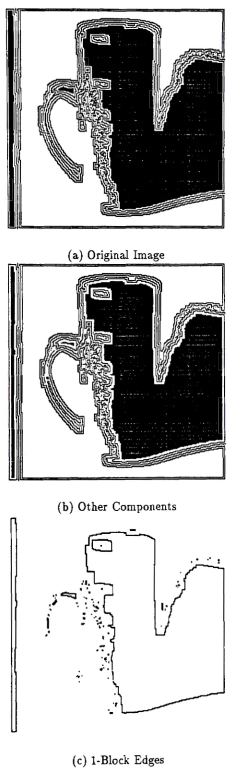
First, the problem of block edge detection is examined using sample pictures in Figure 1 (a)-( c ).
Figure l(a) is a sample image composed of other structures (isolated, inner and network components)
and 1-block edges. It has been separated into other structures in Figure l(b) and 1-block edges in
Figure 1( c). If we restrict the image to the hexagonal grid, is it feasible to perform similar operations
mechanically?
2.1 The Kernel Form of the Hexagonal Grid
To answer this question, it is necessary to analyze how many structuring patterns are required for
block edge detection.
Let X denoted a binary image on the hexagonal grid, x E X be a given point of the image. The
simplest scheme for block edge detection on the hexagonal grid uses seven adjacent grid points (the
kernel form of the hexagonal grid) as the structuring form. The kernel form is a regular form composed
of seven grid points for which one point x is at the centre and another six neighbouring points x0 - x5
are around it. The kernel form can be denoted by ]( ( x) shown in Figure 2. Each point is allowed to
assume values of only 1 or O; seven points have fixed values as a state (structuring pattern), and there
(a) Original Image
(b) Other Components
.
·.
.
·:~ .,
~
..
-. ' ~ .... '!ti
.
:
.
.
-~. ,,.
( c) 1-Block Edges
.
.·K(x) = Xs x X
=
(x .•. X· .•• X1 Xo) - (xs .•. X· ... Xi Xo)2 ' ' " ' ' - ' ' " ' ' '
Xi E {0, l}, 0 ~ i ~ 6, x EX.
Figure 2: The Kernel Form of the Hexagonal Grid
2.2 Different Block Edge Points
For any point x of a binary image on the hexagonal grid, it is a block edge point if it has at least two
neighbouring points in a run which have the same value as x and there is at least one neighbouring
point in opposite value. It is a simple block edge point, if it is a block edge point and all neighbouring
points which have the same value as x are arranged as one run and other neighbouring points with
the opposite value in another run. It is an extensive block edge point, if it is a block edge point and
there are more than two runs of neighburing points in the same value as x.
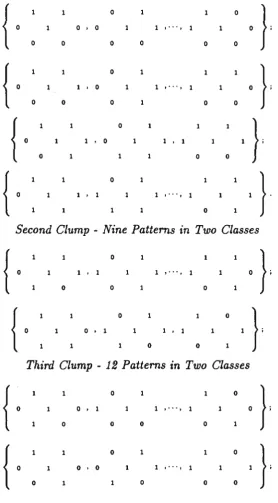
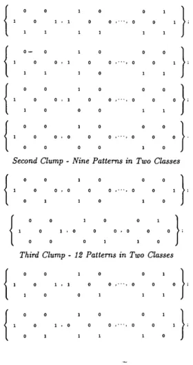
2.3 Three Clumps of Block Edge Patterns
In order to satisfy the requirements of detecting 1-block edges, the following state sets have to be
selected as the structuring patterns. There are eight rotational invariant classes with a total of 45
states in three clumps - first clump: 24 states in four classes for simple block edge patterns; second
clump: nine states in two classes for extensive block edge patterns with two runs (3-1 and 2-2 runs)
and third clump: 12 states in one class for extensive block edge patterns for two runs (2-1 and 1-2
runs) respectively shown in Figure 3. Conversely, for describing 0-block edges, another three clumps
of the conjugate state sets have to be selected as the structuring patterns. There are eight rotational
invariant classes with a total of 45 states too shown in Figure 4.
Because a. block edge is composed of three clumps of states in 16 rotational invariant classes, it is
Structuring Patterns of 1-Block Edges: First Clump - 24 Patterns in Four Classes
{
0 0}
·
0 0 • 0 1 • • 1 0
0 0 0 0 0 0
{
'
1 0
'
}
1 • 0 1 1 • • 1
0 0 0 0 0
{
0 1}
·
0 1 1 • 0 1 • 1 1
0 0 0
{
'
0 1
'
}
1 • 1 1 1 • • 1
1 0
Second Clump - Nine Patterns in Two Classes
{
'
0
'
}
; 1 • 1 1 • • 10 0 0
{
'
1 0 1 0
'
}
;0 • 1 1 1 • 1
0 0
Third Clump - 12 Patterns in Two Classes
{
0 0}
·
0 0 • 1 1 • • 1 0
0 0 0 0
{
'
0 0
'
}
;0 • 0 1 • • 1
0 0 0 0
Structuring Patterns of 0-Block Edges: First Clump - 24 Patterns in Four Classes
{
0 0 0 0};
0 1 • 1 0 0 • • 0 0
{
o- 0 0 0 0}
;
0 0 • 1 0 0 • • 0 0
0
{
0 0 0 0 0};
0 0 • 1 0 0 • • 0 0 0
0 0 0
{
'
0 0 0 0 0
.
}
0 0 • 0 0 0 • • 0 0
0 0 0 0 0
Second Clump - Nine Patterns in Two Classes
{
'
0 0 0 0 0
'
}
; 0 0 ' 0 0 0 • • 0 00 0 0
{
'
0 0 0 0
.
}
;0 1 • 0 0 0 • 0 0
0 0 0 1 0
Third Clump - 12 Patterns in Two Classes
{
0 0 0 0 1}
;
0 1 • 1 0 0 • 0 0 0
0 0
{
'
0 0 0 0
'
}
;0 1 • 0 0 0 ' • 0 0
0 0
patterns. If we could get a simpler organization to identify these block edge states, then it is helpful for
block edge detection to get an efficient algorithm. Therefore, the requirements of looking for efficient
operations of block edge detections force us to investigate proper representations of the state set of the
kernel form of the hexagonal grid. From the above discussion, we can establish the following lemma.
Lemma 2.3.1 For any binary image of the hexagonal grid, if the kernel form of the grid is selected as
the structuring form and three clumps of block edge patterns need to be identified, then it is necessary
to select 90 structuring patterns from its 128 state set. The selected structuring patterns belong to 16
rotational invariant classes and each class contains three to six states.
Proof: No other states can be identified as block edge state from the hexagonal grid in relation to
the kernel form except selected states in Figures 3-4. Three clumps of state sets shown in Figures 3-4
contain all state set relevant to 0 and 1 block edge points. Each number of a class can be counted
directly. D
From an algebraic viewpoint, three operations can be identified to transform the structuring patterns
of block edge detections. The first one is the conjugation which establishes 0 to 1 and 1 to 0 symmetry.
The second one is the number of connections and the third one is the number of branches. Three
conditions play the key role for the problem of block edge detections.
2.4 The Conjugate Classification of the Kernel Form
The conjugate classification of the kernel form of the hexagonal grid is established by Zheng and Maeder
{1992) and further systematic investigations are shown in [Zheng Thesis 1994]. For a convenience in
description, the classification can be briefly described as follows:
The kernel form ]( ( x) of the hexagonal grid is a point x with six neighbouring points around it.
When each point is allowed to assume values of only 0 or 1, there is a total of 128 states corresponding
to unique instances of the kernel form. From the state set Q(K(x)) of 128 states and the inclusion
relation of set theory, we can use a hierarchy of six levels to represent the conjugate classification.
not contain the same state. If we let Q(K(x)) be the root, then the first level can be divided into one
state set G and one conjugate state set
G
dependent on the value of the centre point x, x E { 0, 1}. Thesecond level of 14 nodes
{pG,P
G}
can be distinguished by p, the number of connections, 0 ::; p ::; 6,that is, the number of six neighbouring points with the same value of the centre point. The third level
of 22 nodes
U
G} and {~ G} is related to q which corresponds to the number of branches, O ::; q ::; 3 (thenumber of runs of the six neighbouring points with the same value of the centre point in each state).
The fourth level of 28 nodes {~G'} and
UG'}
has the property of rotational invariant in which any twostates in a node can be congruent by rotation, and s denotes the number of spins, s E { -1, 0, 1 }. Only
six nodes for q = 2 need to be identified using s. The fifth level of 128 leaves
{:G:}
and{:G:}
has asimple relation to the respected state, and r denotes the number of rotations 0 ::; r ::; 6. In short, the
conjugate classification is a hierarchy of six levels: one root, two nodes, 14 nodes, 22 nodes, 28 nodes
and 128 leaves. Each node of the hierarchy is a class of states with 1-5 calculable parameters. The
whole structure of the classification has been represented by (x,p,q,s,r) which denote five calculable
parameters of this classification [Zheng and Maeder 1992]. For convenience, each intermediate node
is called a class too.
2.5 The Proper Level for Block Edge Detections
The hierarchical structure of the conjugate classification provides a :flexible framework for supporting
different applications. It is obvious that x or ( x, p) is not enough to describe the selecting block edge
classes. However, it is possible to use three parameters (x,p, q) for the description.
We need some explanations to determine which level is a proper level of the conjugate classifi.cation
for an arbitrary operation of block edge detections. If states in first to third clumps need to be selected,
it is necessary and sufficient to use the third level: (x,p,q). Owing to this reason, we use the third
level of the conjugate classification to implement required operations, that is, the substructure of the
conjugate classification involving 22 nodes
{:G}
and{:G}.
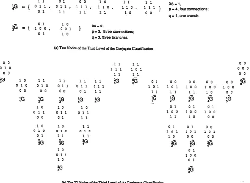
The third level of the conjugate classification is illustrated in Figure 5. Some details of two nodes are
1 1 0 1 0 0 1 0 1 1 1 1 xs.1.
lG
=
{ 0 1 1 • 0 1 1 • 1 1 1 1 1 0 1 1 0 • 1 1 1 } p. 4, four oonnections;0 l 1 l 1 1 1 1 1 0 0 0
q • 1, one branch.
~
0 1 1 0 xs.o;=
{ 1 0 0 0 0 1 -}0 1 1 0 p • 3, three connections;
q • 3, three branches.
(a) Two Nodes of !he Third Level of !he Conjugate C!llsificaticn
0 0 1 1 1 1 0 0
0 1 0 1 1 1 1 0 1 0 0 0
0 0 1 1 1 1 0 0
gG 1 0 1 1 1 1 1 1 1 1 ~
gG
0 1 0 0 0 0 0 0 0 0 o(l0 1 0 0 1 0 0 1 1 0 1 1 0 1 1 1 0 1 1 0 1 1 0 0 l 0 0 l 0 0 8
0 0 0 0 0 0 0 1 1 1 1 l l 1 l 1 1 0 0 0
,G
,G
,G
!G
,G
,G
,G
,G
,G
,G
1 2 3 5 1 2 3 4 5
1 0 1 0 1 0 0 1 0 1 0 1
0 l l 0 l l 0 1 1 l 0 0 1 0 0 l 0 0
0 0 0 l l l 1 1 l 0 0 0
l 0 1 0 l l 0 1 0 1 0 0
0 1 0 0 1 0 0 1 0 l 0 1 1 0 1 1 0 1
0 1 1 1 1 1 1 0 0 0 0 0
kl
~ ~~ ~ ~
1 0 0 1
0 1 1 1 0 0
1 0 0 1
~
~
(b) The 22 Nodes of !he Third Level of !he Conjugate C!llsificaticn
Figure 5: The Third Level of the Conjugate Classification
In order to describe the selected structuring patterns, only
flG,
~G,~G,JG,lG,;G,
~G, ~G,~G, ~G,lG,;G}nodes of the third level of the conjugate classification, are relevant. Their combinations can satisfy
the most applications of block edge detection relevant to the first to third clumps.
Proposition 2.5.1 The third level of the conjugate classification can provide a necessary
representa-tion for the 16 classes of block edge points of the hexagonal grid.
Proof: The third level of structure contains 12 nodes relevant to selected 16 classes that can be
distinguished from each other. It is necessary to support most combinations of these classes. Neither
(x,p),(x,q),(p,q) nor (x),(p),(q) can represent the required classes. So it is necessary for a block
2.6 Three Configurations of Block Edge Detections
Since we can select a subset of 12 nodes from the third level to generate an operation of block edge detections. It is necessary to declare what are three configurations in our investigation.
Let
Ai
orBi
C 9(K(x)) denote the block edge state set of the i-th configuration, 0 ~ i ~ 2. Six block edge state sets can be defined as follows:Ao
{~(;,~(;,~(;,~(;}; (1)Bo
-
{2(;, l _ l _ l _ l _ 3Ci, 4Ci,sli};
(2)A1
{Ao,;Ci};
(3)B1
{Bo,;G};
(4)A2
-
{Ai,ili};
(5)B2
-
{Bi,iG}.
(6)As for the previous investigations for block edge points of three clumps, three configurations correspond the best possibility to use three clumps on the third level of the conjugate classification for block edge detection.
Let
I Ai I
denote the number of states inAi,
we haveIAol -
IBol
= 24; (7)IAd -
IBd
=
33; (8)(9) For convenience in representations on the third level, we use above three configurations to construct six operations for block edge detections.
3 Expressions for Block Edge Detections
3.1
Cellular Logic Computation
For a given configuration
Ai
orBi,
we can use each state in the state set as a mask to representa detecting expression in one of two canonical forms. Let I E 9(K(x)) be a state, Ji E {O, 1},
x{'
=(xiI-
Ji)= (-ixin
Ji)u
(xin
-,Ji) andx;'
1' =(xi= Ji)= (xin
Ji)u
(-ixin
-,Ji)· The detectingexpression for x point needs to contain all variables in K(x). An expression can be denoted by either
CL(K(x),A;) or CL(K(x),B;).
In convenience, let Xs = x and x,,I, E
{O,
1 }, i E{O, .. ·,
6} and let Y; be a detecting function ofthe j-th configuration for 1-block edges and
Y;
be a detecting function of the j-th configuration for0-block edges, j E {O, 1, 2}. We have two expressions.
Y;
-
CL(K(x),A;) (10)-
U1e.A,(nT=oxf');
Y;
- CL(K(x),B;) (11)-
n/EB; Ui:OXi • ·
( 6 ..,/·)It is evident that the first detecting expression determines a 1 block edge point and the second
expressions determines a 0 block edge point on the image. There is one-one corresponding relationship
between a configuration of block edge detection and a detecting expression in cellular logic
compu-tation. However it is well known that there is no simple method to simplify a canonical Boolean
expression into its optimal form when the expression contains rotational invariant classes [Dougherty
1992, Serra 1982]. For most applications, it is most convenient to use two canonical expressions.
Ow-ing to intrinsic difficulties of simplification of cellular logic expressions, it is reasonable to assume that
a running time measurement of a detecting function is proportional to the number of states contained.
3.2 Conjugate Functions for Block Edge Detections
The third level of the conjugate classification uses three invariants: ( x, p, q) representing different
classes of the state set, Two parameters p and q are not Boolean variables. It is necessary to use
For any class of the third level of the conjugate classification, there are three parameters ( x, p, q ):
conjugation, connection and branch, x E {0,1},pE {0,1,···,6} and q E {0,1,2,3}.-Three
configura-tions correspond top= q, p ~ 1 plus q = 2, q = {3, 4} conditions.
Two parameters p and q can be evaluated by following expressions.
5
P - l:(xi=f:x); (12)
i=O
(13)
In order to describe the selected nodes of 1 or 0 block edge points, we can use the following
expressions to project each (x, p, q) index into a 0-1 value.
Let {
=,
=/:,
5, ~} be arithmetic logic operations. For any x and y,l
1, if x=
y; x::y-0, otherwise.
l
1, if x=/:
y; x=f:y0,
otherwise.l
1,
if x 5 y; x5y-0,
otherwise.11,
if x ~ y;x~y
-0,
otherwise.Using four operations plus three Boolean logic operations, we can express all three configurations of
0 or 1 block edges through six functions.
Using the same Y; (or Yi) function as output value for a 1 (or 0) block edge point of the j-th
config-uration and any configconfig-uration Ai (or Bi), let Yi= CT(K(x),Ai) (or Yi= CT(K(x),Bi)) denote the
detection function for the given condition, We have six functions (Type A).
- ( ( x
=
1)n (
q=
1)n
(p=
2))u ( (
x=
1)n (
q=
1)n
(p=
3))u
( ( x
=
1)n (
q=
1)n
(p=
4))u ( (
x=
1)n (
q=
1)n
(p=
5));Yi
- CT(]((x),Ai) (15)-
You ( (
x=
1)n (
q=
2)n
(p=
4));Y2
=
CT(]((x ),A2)
(16)-
Yiu
(x=
1)n
(q=
2)n
(p=
3));Yo
-
CT(K(x ), 80) (17)-
( ( x"I
1)u (
q"I
1)u
(p"I
2))n ( (
x"I
1)u (
q"I
1)u
(p"I
3))n
( ( x
"I
1)u (
q"I
1)u
(p"I
4))n ( (
x"I
1)u (
q"I
1)u
(p"I
5));Yi
- CT(]((x ),Bi)
(18)=
Yon ( (
x"I
1)u (
q"I
2)u
(p"I
4));Y2
-
CT(K(x),81) (19)-
Y1n ( (
x-I
1)u (
q-I
2)u
(p-I
3)).The six functions can be simplified further (Type B). That is,
Yo
- CT(K(x ),Ao)
(20)=
( x=
1)n (
q=
1)n
(p ~ 2);Y1
-
CT(K(x),A1) (21)=
You ( (
x=
1)n (
q=
2)n
(p=
4));Y2
=
CT(K(x ),A2)
(22)=
Yo u ( (
x=
1)n (
q=
2)n
(p ~ 3));Yo
-
CT(]((x),Bo) (23)=
((x"I
1) U (q"I
2) U (p<
2));Y1
-
CT(K(x),Bi) (24):::..
Y2 - CT(K(x),82 ) (25)
- Yo
n ( (
x :j:. 1)u (
q :j:. 2)u
(p<
3)).Compared the simplified expressions (Type B) and original expressions (Type A), it is evident
that two functions Yo, Yo can be simplified equivalent to involving one class and another two functions
Y2, Y2 can also be reduced to contain two classes. Two intermediate functions y1 , jj1 can be expressed
as two classes too. These situations inform us that not only could conjugate functions concentrate
configurations using classes, but also their expressions could be further simplified depending on specific
distributions among involving classes.
For three configurations, six functions from two cellular logic expressions are equivalent to six
functions of the conjugate expressions.
Proposition 3.2.1 The six detecting functions of the cellular logic expressions of three configurations
for block edge detections coTTespond to the six detecting functions of the conjugate expressions.
Proof: A pair of two corresponding functions contains the same state set. Multiple variables determine
the same output values. They can be verified directly. D
Using the proposition, we have following corollaries.
Corollary 3.2.2 x is a 1-block edge point of the i-th configuration, if Yi - 1; otherwise Yi - 0,
0 ::; i ::; 2.
Corollary 3.2.3 x is a 0-block edge point of the i-th configuration, if
Yi
-
0; otherwiseYi
-
1,0 ::; i ::; 2.
Three functions correspond to 1 block edge points and another three functions determine 0 block
edge points.
4
Complexity Analysis for Block Edge Detections
There are obvious differences between a cellular logic function and a conjugate function. A cellular
Boolean plus arithmetical variables and logic plus arithmetical logic operations. In modern computer,
an instruction takes a unit time either a logic, arithmetical logic or simple arithmetical operation. In
relation to this equivalence, we can just calculate how many binary operations are required in each
function. Using these complexity measurements, it is sufficient to compare two corresponding functions
theoretically. Let TB denote a unit time for a binary operation, Tp, Tq denote the number of binary
operations evaluating p and q parameters, T(CT(K(x),A)) denote the number of binary operations
involved in CL and CT equations, N = IAil = IBd be the number of states and n = llAill = llBill be
the number of classes. We have following equations.
T( C L(K(x ), Ai)) T( C L(K(x ), Bi)) (26)
-
14x
Nx
iB' 0 ~ i ~ 2;To( CT( K( x ), Ai)) T(CT(K(x),Bi)),O ~ i ~ 2; (27)
-
ip+
Tq = 14 X TB+
14 X TB28 X TBj
T1 (CT( K( x ), Ai))
-
T(CT(K(x),Bi)),O ~ i ~ 2; (28)-
7 X n X iBiT( CT(K(x ), Ai))
-
T0 ( CT)+
T1 (CT) (29)- (28
+
7 X n) X iB•Using T(CL) and T(CT) measurements, we can investigate a speed-up ratio between two
equa-tions. Let SpfL=CT
=
T(CL)/T(CT) be a theoretical speed-up ratio of CL and CT for the iconfigu-ration. Three configurations correspond three speed-up ratios: No = 24, no = 4; N1 = 33, n1 = 6 and
N2 = 45, n2 = 8
SpfL:CT 14 x
Nd (
28+
7 x ni)2 x Ni/(4
+
ni)·Sp~L:CT - 2
x
24/(4+
4)='
6;Spf L:CT 2 x 33/( 4
+
6) = 6.6;(30)
(31)
SpfL:CT = 2 x 45/(4
+
8) = 7.5. (33) From the equation of a speed-up ratio for two schemes, it is evident that the conjugate functioncould have a speed-up ratio 6-7.5 faster than the corresponding cellular logic function. To use further
simplified forms of the equations, a higher speed-up ratio can be achieved. We have N0
=
24, n0 = 1;Ni
= 33, n1=
2 and N2 = 45, n 2 = 2.2x24/(4+1) = 9.6;
SpfL:CT - 2 x 33/(4
+
2)=
11;Sp~L:CT - 2
x
45/(4+
2) = 15.In general, three configurations have a theoretical speed-up ratio 6-15.
5 Using the Conjugate Functions
(34)
(35)
(36)
In order to illustrate the advantage of the conjugate functions for block edge detections, two sets
of sample pictures of binary images for three configurations of block edge detections are shown in
Figure 6 and Figure 7 for 1-block edges and 0-block edges respectively in Appendix A. The pictures
are generated from an implemented prototype of the conjugate transformation of the hexagonal grid
[Zheng and Maeder 1993]. The conjugate transformation can support any combination of the selected
classes from the 22 nodes of the third level of the conjugate classification. In Figures 6-7, pictures
(b )-( c) illustrate three configurations for 1 (or 0) block edges respectively. Pictures (b) are simple
block edges; both pictures ( c) contain more block edge points and two pictures ( d) provide the most
details of block edge points. A specific application can correspond to one of three configurations.
Because of the capability of the class representation to efficiently identify states, the implementation
of the conjugate transformation on the hexagonal grid is very efficient. A speed-up ratio 6-15 for real
measurements, compared with the same activity (0 or 1 block edge detection) performed by a standard
implementation of cellular logic functions, can be observed. Both theoretical and real speed-up ratios
Table 1: Time Measurements of Two Schemes
Function ni Ni CT CL SpcL:CT SpCL:CT Sample
Full Edges 1 1 86 38 0.44 0.4 Fig.6&7(e)
One Class 1 6 86 230 2.6 2.4
i=O 4 24 146 970 6.6 6 Fig.6&7(b) Type A
i=O 1 24 86 970 11.2 9.6 Fig.6&7(b) Type B i = 1 6 33 186 1367 7.3 6.6 Fig.6&7( c) Type A
i = 1 2 33 105 1367 13 11 Fig.6&7( c) Type B
i = 2 8 45 226 1920 8.4 7.5 Fig.6&7( d) Type A
i = 2 2 45 105 1920 18.2 15 Fig.6&7( d) Type B
Note: ni is the equivalent number of classes for the i-th configuration, Ni is the number of involved states, CT
is the average number of time units taken by a conjugate function, CL is the average number of time units taken by a cellular logic function, SpcL:CT is equal to CL/CT for a speed-up ratio of real measurements,
SpCL:CT is a speed-up ratio for theoretical measurements and Sample indicates sample figures.
of running times of two compared programs on Model: CMN-BOOl, !RIX 4.0.5 System V, Silicon
Graphics Iris 4D /25. The unit of the measurement time is 1/60 second.
6 CONCLUSION
From both representation and implementation, the proposed solution of three configurations of block
edge detections based on conjugate functions is superior to cellular logic functions in the condition of
representing composed classes in multiple structuring patterns. Using the proper class information, the
48, 66 and 90 states of the structuring patterns for block edge detections can be drastically reduced to
simple expressions. This detection, therefore, provides a general structural description of relationships
analysis and processing operations of binary images on the hexagonal grid.
Acknowledgements: The author would like to express gratitude for Mrs. Patrizia Rossi for editing and proofreading this paper.
References
Dougherty E.R. (1992). An Introduction to Morphological Image Processing, SPIE Optical Engineering Press.
Golay M.J.E. (1969). "Hexagonal Parallel Pattern Transformations" IEEE Trans. Comput. Vol.18, pp733-740.
Kong T.Y. and Rosenfeld A. (1989). "Digital topology: Introduction and survey" Comput. Vision Graphics Image Processing. 48, pp357-393.
Pitas I. a.nd Venetsanopoulos A. (1989). "Morphological Shape Decomposition," IEEE Trans. Pattern Anal. Machine
Intell., Vol. 11, No. 7, July, 1989.
Preston Jr K. and Duff M.J.B. (1984). Modern Cellular Automata: Theory and Application Plenum Press, New York.
Rosenfeld A. (1979). "Connectivity in digital pictures", JACM, 17, pp146-160.
Shapiro L., MacDonald R. and Sternberg S. (1987). "Ordered Structural Shape Matching with Primitive Extraction
by Mathematical Morphology," Pattern Recognition, Vol. 20, No. 1, 1987.
Zheng Z.J. and Maeder A.J. (1992). "The Conjugate Classification of the Kernel Form of the Hexagonal Grid", Modern
Geometric Computing for Visualization eds by T.L. Kunii and Y. Shinagawa, Springer-Verlag, pp73-89.
Zheng Z.J. and Maeder A.J. (1993). "The Elementary Equation of the Conjugate Transformation for Hexagonal Grid",
Modeling in Computer Graphics, eds by B. Falcidieno and T.L. Kunii, Springer-Verlag, pp21-42.
Zheng Z.J. (1993a). "A Necessary Condition for Block Edge Detection of Binary Images on the Hexagonal Grid",
Communicating with Virtual Worlds, eds by N. M. Thalmann and D. Thalmann, Springer-Verlag, pp553-566.
Zheng Z.J. (1993b). "An Efficient Scheme for Simple Network Detection for Binary Images on the hexagonal Grid,"
sub-mitted to IEEE TENCON '94, Special Session On COMPUTER GRAPHICS & APPLICATIONS, and Technical
Report No. 93/195, Department of Computer Science, Monash University, 22p.
Zheng Z.J. {1993c), "Three Configurations of Network Detections for Binary Images of the Hexagonal Grid," submitted
to Computer Graphics lnternational'94, and Technical Report No. 93/194, Department of Computer Science,
Monash University, Dec. 1993, 24p.
Appendix A
! .
(a)
(b)
Figure 6: Sample Pictures of Black-ground (a)-(e).
(a) original image (256 by 256), (b)-(e) sample
images; (b)
Ao
Block Edge; ( c) A1 Block Edge;( d) A2 Block Edge; ( e) Full Edges for 1 Points.
~ .~ ...
.,,_;
..
~
.
.
~
- .
...
.
\,.tiL
,
...
. , ·,
.
.
·~
(c)
(d)
' I
l
!
i 1 ! ,.
.
"I
§
(a)
(b)
Figure 7: Sample Pictures of White-ground
(a)-( e). (a)-(a) original image (a)-(256 by 256), (a)-(b )-(a)-( e) sample
images; (b) 80 Block Edge; (c) 81 Block Edge; (d)
82 Block Edge; ( e) Full Edges for 0 Points.
(c)
(d)