Technical Efficiency of Small Scale Fish Farming in Kiambu County

TECHNICAL EFFICIENCY OF SMALL SCALE FISH FARMING IN KIAMBU COUNTY

BENARD KIPLAGAT YEGON

A RESEARCH PROJECT SUBMITTED TO THE SCHOOL OF ECONOMICS IN

PARTIAL FULFILMENT OF THE REQUIREMENT FOR THE AWARD OF

MASTERS OF ECONOMICS (FINANCE) DEGREE AT KENY ATTA UNIVERSITY

JULY 2015

DECLARATION

This is my original work and has not been presented for a degree award in any other university.

Signature ~ Date

\?\<:

l

1;\~?\S"

Benard Kiplagat Yegon KI021 CTYIPT/21506/2010

This project is s bmitted with our approval as supervisors:

Signature... . Date

L6.lt[.I}~

.

Dr. Dianah Mukwate Ngui Senior Lecturer

Department of Econometrics and Statistics Kenyatta University

Signature ... ~.... .Date ..

lo.~/!:.?(j.=

Dr. Aflonia N~'l~~:' Lecturer

DEDICATION

ACKNOWLEDGEMENT

ABSTRACT

\

TABLE OF CONTENTS

DECLARATION i

DEDICATION .ii

ACKNOWLEDGEMENT : .iii

ABSTRACT iv

LIST OF TABLES viii

LIST OF FIGURES ix

LIST OF ACRONYMS AND ABBREVIATIONS x

OPERATIONAL DEFINITION OF TERMS xi

CHAPTER ONE : : 1

INTRODUCTION 1

1.1Background of the study 1

1.2 Statement of the Problem 7

1.3Objectives of the study 9

1.4Research Questions 9

1.5Significance of the study 9

1.6 Scope of the study 10

1.7 Organization of the study 10

CHAPTER TWO 11

LITERATURE REVIEW 11

2.1 Introduction 11

2.2 Theoretical Literature 11

2.2.1 Scientific Management theory 11

2.2.2 Neoclassical Production Theory 12

2.2.3 The Classical Production Theory 13

2.2.4 The Classical Production Function 14

2.3. Technical Efficiency 16

2.3.1Farrell's Measure of Efficiency 16

2.4 Empirical literature 19

2.6 Overview of Literature 25

CHAPTER THREE 28

RESEARCH METHODOLOGy : 28

3.1 Introduction 28

3.2Research design 28

3.3Theoretical Model · 28

3.4 Empirical Model.· 29

3.5 Definition and measurement ofthe variables 31

3.6 Study area 31

3.7Data and sampling technique 32

3.8 Data collection procedure 32

3.9 Instrument Validity and Reliability 33

CHAPTER FOUR 34

EMPERICAL FINDINGS 34

4.1 Introduction 34

4.2 Summary statistics of Small Scale Farmers in Kiambu County 34 4.3 Determining Technical Efficiency of Small Scale Fish Farmers 38

4.3.1 Test Statistic 38

4.3.2 Technical Efficiency of Small Scale Fish Farmers in Kiambu County .40 4.3.4 Level of Technical Efficiency among the Small Scale Fish Farmers in Kiambu

County 43

4.3.5 Technical Efficiency Distribution and Household Characteristics .45 4.4 Determinants of technical efficiency in the small scale fish farming in Kiambu

County 46

4.4.1 Inefficiency model 46

CHAPTER FIVE 50

SUMMARY, CONCLUSIONS AND RECOMMENDATIONS 50

5.1 Introduction 50

5.2 Summary 50

5.3 Conclusion 51

5.6 Areas

for

Further

53

REFERENCES 54

APPENDICES 1

64

QUESTIONAIRE

FORM

64

LIST OF TABLES

Table 1.1 Fish Production and Import Volumes of Kenya 5

Table3.1 Definition of Variables 31

Table 4.1: Summary Statistics of Small Scale Farmers in Kiambu County 35

Table 4.2: Log Likelihood Test for Hypothesis and Functional Forms 39

Table 4.3: Maximum Likelihood Estimates ofthe Stochastic Frontier Production Function for

Small Scale Farmers 40

Table 4.4: Frequency Distribution of Technical Efficiency (%) in Small scale Fish Farming ..43

Table 4.5: Summary of technical efficiency by household characteristics .45

/

LIST OF FIGURES

Figure 1.1 Fish Farming Data 2003-2010 .4

/

LIST OF ACRONYMS AND ABBREVIATIONS

FAO Food Agricultural Organization

ERS Economic Recovery Strategy

PRSP Poverty Reduction Strategy Paper

GOK Government of Kenya

ESP Economic Stimulus Programme

MT Metric Tonnes

HA Hectares

NPV Net Present Value

IRR Internal Rate of Return

SFA Stochastic Frontier Analysis

SPF Stochastic Production Frontier

DFA Deterministic Frontier Analysis

MOLFD Ministry of Fisheries Development

MLE Maximum Likelihood Estimate

DEA Data Envelopment Analysis

DMU Decision Making Unit

ADP Agricultural Development Programmes

LGAs Local Government Areas

Efficiency

Inputs Output Pond Fingerlings Inefficiency Aquaculture

OPERATIONAL DEFINITION OF TERMS

measure of how well resources are used to produce a certain level of output

resources required to produce output (kgs of fish) kilograms of fish harvested by the farmer

area for producing or rearing fish seed of fish or young ones of fish

CHAPTER ONE

INTRODUCTION

1.1 Background of the study

The growing human population and reports of large numbers of malnourished people

especially in the developing countries have made the need for food production a major

worldwide matter of concern. It is estimated that about 870 million people in the world

do not have adequate access to food and 852million of these are in developing countries

(FAD, 2012). Most of these countries are characterized by low economic growth, low agricultural production, recurring political upheavals, persistent drought, environmental

degradation and severe poverty. Given this scenario, it's imperative to focus on new

ways of providing the people with alternative means of getting food sufficiency. The

three main groups of human activities that contribute to food production are:

agriculture, aquaculture and fisheries.

In Kenya, fisheries sector plays a significant role in the social and economic

development through the sector's positive contribution to employment creation, revenue

generation and food security - all of which are crucial for the attainment of the

Millennium Development Goals and achievement of Kenya vision 2030(Fisheries

Department, 2010).The national fish production comes from three major sources

namely; Inland lakes and rivers (capture fisheries), Marine and fish farming. The global

and about one third of them being either depleted or overexploited (FAO, 2003). According to FAO (2004), deterioration of global fisheries is raising significant concern, mainly because an estimated one billion people, mostly in low-income countries, depend on fish as their primary source of protein. Similarly, Kenya's Lake Victoria which has been supplying 90% of total national fish production has been recording declining fish stock. The production from the lake declined from 143,908 metric tonnes in the year 2006 to 124,643 metric tonnes in year 2013(Fisheries Department, 2011; Government of Kenya, 2014). This scenario calls for prudent management of the fish stocks in the natural sources by expanding fish production in

the country through aquaculture.

Fish farming in Kenya started in 1900s when colonialists stocked trout in rivers between 1910 and 1912 for sport fishing (Vernon and Someren, 1960).The activity was seen as one of the ways of promoting protein food supply, creation of employment opportunities, and supplementing the capture fisheries in-terms of supply of fish, which currently is acutely threatened. Though aquaculture was introduced in Kenya at the beginning of the last century, the production has not picked up considerably considering

(

technology and fish breeding practices and unknown investment return-rates (Manyala and Ngugi, 2004).

This situation was even made worse because the Kenyan fisheries sector had operated without a comprehensive policy and legal framework on fisheries since 1963. However fisheries production and management measures were from time to time mentioned in various policy documents. Fundamental among these include : The National Food Policy (1981 and 1994) in which the importance of fish as a nutritious food commodity was emphasized, the District Focus for Rural development Policy (1985) that required all districts to have fisheries presence irrespective of their fisheries potential, the

Poverty Reduction Strategy Paper (PRSP) of 2001 that introduced a social

responsibility and poverty reduction element into the fisheries agenda, the Economic Recovery Strategy (ERS) for wealth creation and employment (2003-2007)into which the PRSP evolved that recognizes the contribution made by fisheries to local incomes, subsistence and nutrition.

information on fish farming technology and breeding practices of fish. This is

exemplified by the fact' that in the year 2010 there were only 4,742 fish farmers in

Kenya with 7,471 ponds producing 12,153metric tonnes of farmed fish (Figure 1.1).

14,000

12,000

10,000

i='

~ 8,000

-

_.•..

•••

6,000 III

::::J

a

4,000

2,000 _{1,012 1,035 1,047 1,012}

12,153

4,895 4,452

4,245

2003 2004 2005 2006 2007 2008 2009 2010

Year

Figure 1.1:Aquaculture production in Kenya from the year 2003-2010

Source: Fisheries Statistical Bulletin, (2012)

The figure shows that production from aquaculture remained relatively low for the

seven years (2003-2009). However with the introduction of Economic stimulus

programme in 2009 the output from fish farming improved to above 12,000metric

tonnes. According to Fisheries Department, the contribution of farmed fish at that time

Fish farming received a major boost in the year 2008 when the government identified it as one of the activities to be funded in the Medium Term Expenditure Framework (MTEF) budget of the year 2009 through the Economic Stimulus Programme (ESP). The implementation of this programme saw the increased hectares of land under fish farming from 722 hectares to 14,076 hectares (G.O.K, 2012). The output offish farming during this period increased from 4,245 to 21,487 metric tonnes accounting between 3 and 16% of total domestic fish production in this period (G.O.K, 2012).

However on a global scale Kenya's aquaculture production is still insignificant accounting for 0.09% of the world production (FAO, 2012; Rothuis

et al.,

Table 1:1 Fish production and import volumes offish in Kenya

Year 1961-1970 1971-1980 1981-1990 1991-2000

2001-2010

Yearly average 24,846 37,368 117,294 188,018 143,662

Production

(MT)

Annual average 2,230 3,878 6,080 8,441 16,244

Import (MT)

The table shows that the yearly average fish production in the country increased from

24,846 to 188,018 metric tonnes then declining to 143,662 metric tonnes. On the other

hand annual average import of fish steadily increased from 2,230 to16, 244 metric

tonnes .Thisshows an increasing supply gap in Kenya meaning consumption of fish is

outpacing production. These calls for attention either through improved production

techniques and attain self-sufficiency or continue meeting the deficits through

importation. The second option is not attainable in the long run considering the fact that

foreign exchange is limited in Kenya which is still relying on importing other essential

commodities like drugs and capital goods. To address this issue of increasing demand

the Kenya government stepped up efforts to increase production of fish by extensively

promoting fish farming in high potential areas.

Kiambu County in central Kenya was identified as one of the fish farming potential

areas because of its climatic conditions that are suitable for fish farming. The county is

densely populated with majority of the inhabitants owning less than an acre piece of

land (G.O.K, 2009)

Fish farming can easily be integrated with other agricultural activities since it requires a

small area to construct the fish pond. Similarly there were reports that coffee and tea

which had for a long time been the main source of income for the region were faced

with international marketing challenges and farmers were contemplating uprooting the

crops. Fish farming was seen to be one of the ways of diversifying the economic

activities, employment creation, and protein food supply in the county. According to

Fisheries County Statistical data of 2011 and 2012, Kiambu County produced 1217 and

production in Kiambu region if only the challenges such as lack of prerequisite

information on aquaculture, affordable credit facilities, inadequate supply of quality fish seed, extension support, lack of comprehensive policy on aquaculture, lack of capacity

to explore market forces, as well as the presence of inefficiency are overcome(Mbugua,

2008). Predominantly, the level of inefficiency of utilization of available resources for

fish farming has remained an unanswered question in the quest for increased fish

production in Kiambu County. It is against this background that the present study was undertaken to examine the factors influencing technical efficiency of fish farming in

Kiambu County.

1.2 Statement of the Problem

Kenya imports a lot of fish and fishery products, for instance a total of 16,244 metric tonnes offish and fishery products were imported between 2003 and 2010 (FAO, 2011).

The increasing demand is largely related to people-shifting from animal protein to fish

protein and increasing tourism activities in the country (FAO, 2010).

Fish farming in Kenya is carried out in earthen ponds measuring 300m2; the productions in these ponds hardly exceed

1.04kg/m

/year

Department, 2010). In Kiambu County, this promotion was mainly done through

demonstrations, farmer trainings, provision of fingerlings and credit to farmers.

Despite the extensive promotion of fish farming, the production has not changed

significantly. In the year 2011 and 2012, Kiambu had a total of 4015and 4273 ponds

producing 1217 and 1336 tonnes of fish worth Ksh 288million and Ksh 311million

respectively (Fisheries Department, 2012). The County statistical data of 2013 shows that Kiambu County produced 2,820 MT which is 6 percent of the total fish produced in

Kenya compared to potential of producing 10 to 15 percent of the total national

production. The farmers in the County are reported to be producing between 0.05 -1.04kg/m2/year as compared to 3to 5kg/m2/year that the Fisheries Research Institutions

recommend (Fisheries Statistical Bulletin, 2012).

This therefore means the increasing output of fish being witnessed in Kenya can be

attributed to the increased number of hectares under fish farming but not improved fish pond productions. Studies have been done on efficiency in livestock and crops

production in Kenya and many have dwelt on the efficiency on crops and none has

dwelt on fish farming. (See for instance Kuria

et

al.,

et

al.,

level of technical efficiency among the fish farmers in the county and analyze the

1.3 Objectives of the study

The general objective of this study is to analyze the level of technical efficiency among

the small scale fish farmers in Kiambu County.

Specifically, the study seeks to:

(i) Estimate the level.of technical efficiency among the fish farmers in Kiambu County.

(ii) Analyze the determinants of technical efficiency in the fish farming enterprise in

Kiambu County.

1.4 Research Questions

(i) What is the level of the technical efficiency among the small scale fish farmers in

Kiambu County?

(ii) What are the determinants of technical efficiency of small scale fish farming in

Kiambu County?

1.5 Significance of the study

Understanding the factors that determine technical efficiency of the small scale fish

farming can enable improvement in efficiency and consequently the profitability of fish

farmers and achieving self-sufficiency in food protein supply. To achieve an economic

optimum output and thus profitability, resources have to be optimaliy and efficiently

utilized. An efficient fish farming industry will not only help to ease the pressure in the

fishing on the inland lakes and rivers but also create employment opportunities to

Kenyans and improve the revenues to the government. Examination of technical

efficiency of the fish farming will make it possible for fishery managers to determine to

base and available technology. Further, the findings of this study will add to the current

body of knowledge on the technical efficiency of small scale fish farming.

1.6 Scope of the study

This study will focus on examining the level of technical efficiency, factors affecting

the technical efficiency of small scale fish farmers in Kiambu County since its one of

the greatest production potential areas due to its favorable geographical features. The

study will use structured questionnaire to collect data from the fish farmers on the

production information, market information and demographic information. The

technical efficiency will be measured in the twelve sub counties of Kiambu over the

period 2009- 2012. This is the period when the government supported the fish farming

through the Economic Stimulus Programme.

1.

7

The remaining part of this proposal is structured as follows; Chapter two presents a

literature review addressing the various aspects of efficiency in production and how

they are inter-linked as well as the measurement of technical efficiency. It outlines past

studies relating to efficiency of production. Chapter three presents a theoretical model

and proceeds to outline an empirical model for technical efficiency and the factors that

influence the technical efficiency. It concludes with a description of the data that will be

used in the study, including the source and how they will be collected. Chapter four

presents the data and discusses the empirical findings of the study while Chapter five

CHAPTER TWO

LITERA TURE REVIEW

2.1 Introduction

This chapter reviews relevant literature on efficiency. It presents a review of theoretical

literature, the techniques of efficiency measurement and empirical literature. The final

section presents determinants of technical efficiency and overview of literature.

2.2 Theoretical Literature

This section discusses theories of production, concept of production functions, technical

efficiency and its measurement.

2.2.1 Scientific Management theory

According to the scientific management theory, the occupations involved in the design

and fabrication of products were gradually split into more and more specialized

professions (division of work). One of its first advocates was Scottish economist Adam

Smith. In the book The Wealth of Nations (1776) Smith pointed out how specialization

tends to develop skill, dexterity, and innovations. Moreover, it saves the time lost in

changing from one kind of work to another. To this list of blessings English

mathematician Charles Babbage (in the book On the Economy of Machinery and

Manufacturers, 1832) added that dividing the task into short operations allows paying

lower wages for the easier tasks. In 1913, Henry Ford put the work division theory in

practice and introduced an assembly line in his car factory, thus reducing the time to

assemble a car from 12hours and 28 minutes to one hour and 33 minutes.

steer daily work so that the targets are met

.

The limitation of the theory is the idea of

looking at production only from labour point of view

.

From economics

,

production

encompasses quite a number of 'variables hence this theory is not applicable for the

current study.

2.2.2 Neoclassical Production Theory

Neoclassical theory argues that Profit is determined by the level of the marginal

productivity of capital, and the wage of workers is determined in a similar way by the

marginal productivity of labor

.

Therefore if a union succeeds in raising the workers'

wage, the inevitable result will be unemployment

.

In

tandem with this new theory of

wages and profits Pareto first dismissed the theory of Utilitarianism which called for

redistributing income, and then developed a new definition of economic efficiency to

replace it

.

According to Pareto's definition

,

the higher union wage results in economic

inefficiency. Although entirely different from Ricardo's theory of profits and wages

,

the

neoclassical theory of profits and wages is an application of another of Ricardo

'

s

theories that

'

of land rent, and this is how neoclassical economics got its name.

According to Ricardo

,

parcels of land differ in their fertility. The most fertile land is

put into production first, and as agricultural production expands less and less fertile

parcels are added; the rent for less fertile parcels is lower than the rent for more fertile

land.

Neoclassical economists argue that the process of adding labor and capital when

industrial production is expanded is similar.

As industrial production expands,

/

assumes that the productivity of each additional worker, which is her marginal product,

diminishes. Neoclassical economics assumes that the employer hires workers one by

one. When she considers whether to hire an additional worker she compares the value

of that worker's marginal product to the wage. As long as a worker's value of marginal

product exceeds the wage, the worker is hired. But because the marginal product is

diminishing, eventually so many workers will have been hired that the value of the

marginal product of an additional worker would be less than the wage. At this point the

hiring will stop. Of course, if at this point the wage rate were raised, some workers

would get fired, because the value of the marginal product of at least some workers

would be below the new wage. Thus, if unions push the wage higher, some workers

would become unemployed, a situation that is not only painful to these workers but is

also Pareto inefficient.

The process of hiring capital is exactly the same. A unit of capital

is

value of the marginal product of capital exceeds the rental price of capital and the

process stops when, because of the decreasing marginal productivity of capital, the

value of the marginal product of capital becomes lower than the rental price. This

theory looks at production broadly in terms of profit and cost which the current study in

not concerned with and hence the theory is not applicable.

2.2.3 The Classical Production Theory

Classical economists postulated the identical production function, which can be written

as Y = f(K, L, N, S) which means that output depends on the stock of capital, labour

'Lam\'

\

~

t*

n

a

s

'1.n

e ~

u

PJ

>l

y

0

1

Kn

ow

n

and econ.omlc~

\\

y

tu

\

res

ou

rce

"

tbi's

seems like the right thing to do as it is not the amount of cultivable land and its fertility

that determines the national output but the total supply of known and usable natural

resources.

Most of the other classical economists, except for'Adam Smith, seem to believe that the

production function is linear and homogeneous, which implies that it has constant

returns to scale meaning that on doubling the quantities of all the factors of production

output would double. Adam Smith, on the other hand, believed in increasing returns to

scale on account of improved division of labour. In case the term land is restricted to

cultivable land only, the supply of which is a fixed amount, then the question to be

answered would be as to how the output would respond to an increased supply of labour

with a fixed supply of land. This theory is relevant to the study and will be relied

heavily on the study mainly the production function.

2.2.4 The Classical Production Function

A production function (also commonly referred to as the pr ducti n fr ntier) i ften

used to illustrate the technical relationship between inputs and outputs in the production

process. The production function represents the maximum level of output attainable

from alternative input combinations (Coelli et al., 2005). The classical production

function (assuming only' a single output is produced from various inputs) can be

specified as:

Where q represents output and X=(Xl,X2 ...XN)' is an Nx1 vector of inputs used in the

farm.

The function f (.) is the production frontier and equation 2.1 gives the upper boundary

of T. Given the input x, the maximum production output q=f(x) can be achieved. In the

form ofmaximization the production frontier is expressed as:

f(x)=max{q : T(x, q}2:0 2.2.

The production frontier serves as the standard against which to measure technical

efficiency. It should contain only the efficient observations. It's assumed in production

theory that the production function has the following properties: No negativity: the

value of f(x) is a finite non-negative, real number. Weak essentiality: the production of

positive output is impossible without use of at least one input. Non decreasing in x

(monotonicity): Additional units of an input will not decrease output.ie if x°2:xl then

f(xo)2:f(xl). If the production function is continuously differential monotonicity implies

all marginal products are non-negative. Concave in x: any linear combinations of

vectors XOand x' will produce an output that is no less than the same linear

combinations of ftx") and f(xl).

Nonetheless, in practice these properties are not exhaustive and may not be universally

maintained. For instance, excess usage of inputs might result in input congestion, which

relaxes the monotonicity assumption. Also, a stronger essentiality assumption often

applies in cases where each and every input included proves to be essential in a

function (i.e., no restrictions imposed except theoretical consistency) is another

desirable feature in order to allow data to capture information on critical parameters.

2.3. Technical Efficiency

A producer is technically efficient if an increase in any output requires a reduction in at

least one other output or an increase in at least one input, and if reduction in any input

requires an increase in at least one other input or a reduction in at least one output

Koopmans, (1951). Thus a technically inefficient producer could produce the same

outputs with less of at least one input or could use the same inputs to produce more of at

least one output.

Farrell (1957) .introduced measure of technical efficiency. His measure of technical efficiency is defined as one minus the maximum equiproportionate reduction in all

inputs that still allows continued production of given inputs. A score of unity indicates

technical efficiency because no equiproportionate input reduction is feasible and a score

less than unity indicate technical inefficiency. According to Farrell (1957), measure of

technical efficiency can be obtained by using input and output without introducing

prices of these inputs and outputs.

2.3.1Farrell's Measure of Efficiency

According to Farrell (1957), measure of technical efficiency can be obtained by using

input and output quantity without introducing prices of these inputs and outputs.

and pure technical efficiency. However this study will be limited to focusing only on technical efficiency.

In the figure 2.2 below, observation A uses two input factors to produce a single output.

SS' is the efficient isoquant estimated with an available technique. Point B on the

isoquant represents the efficient reference of observation A. the technical efficiency of a

production unit operating at A is most commonly measured by the ratio:

TE= OB/OA,

This is equal to one minus BAlOB. Itwill take a value between zero and one, and hence an indicator of the degree of technical inefficiency of the production unit. A value of

one indicates the firm is fully technically efficient. For example the point B is

technically efficient because it lies on the efficient isoquant. If the input price ratio,

s

L(y)

-

~~

__

-

Sl

W

I

o

Figure 2.3 technical and allocative efficiencies

Source: Farrell, (1995)

The allocative efficiency (AE) of a PU operating at A is defined to be the ratio:

AE= OC/OB

Since the distance CB represents the reduction in production cost that would occur if

production were to occur at the allocative and technically efficient point E, instead of

the inefficient point B.

The total economic efficiency (EE) is defined to be the ratio:

EE=OC/OA

Where the distance CA can also be interpreted in terms of a cost reduction. The product

of technical efficiency and allocative efficiency measures provide the measure of

2.4Empirical literature

Weir (1999) and Weir and Knight (2000) using the stochastic frontier analysis studied

the impact of education externalities on production and technical efficiency of farmers

in rural Ethiopia. They found evidence that the source of externalities to schooling is in

the adoption and spread of innovations that shift out the production frontier. Mean technical efficiency of cereal crop farmers ware 0.55, for instance a unit increase in

years of schooling increases technical efficiency by 2.1 percentage points. One

limitation of the Weir (1999) and Weir and Knight (2000) is that they investigated the

levels of schooling as the only source of technical efficiency. However the current study

studied several variables which could be affecting technical efficiency.

Kuria et al., (2003) examined the technical efficiency associated with rice production in

Mwea Irrigation Scheme in Kenya using the stochastic frontier method of estimation.

The study compared two groups of farmers, one group consisting of farmers growing a

single crop of rice in a year and the other growing a double crop of rice in a year.

Empirical results indicated that farmers growing a single crop of rice were more

technically efficient than those growing a double crop of rice in a year. Farmer's education level and farming experience as well as availability of credit and extension

facilities were found to be significant variables that influence technical efficiency.

However the assumption that farmer's specific characteristics as well as institutional

Okechi(2004) evaluated the profitability assessment of Catfish Fish farming in Lake

Victoria Basin using the Net Present Value (NPV), Internal Rate of Return (IRR),

payback period and Debt Service Coverage Ratio. A sensitivity analysis on stocking

density, survival rates, cost of feed, cost of fingerlings and sales price was also

conducted. The findings of the analysis indicate that catfish farming is financially

feasible. The results obtained indicate a positive NPV and acceptable IRR and a

payback period of five years. A debt service coverage ratio of more than 1.5 was

obtained thus indicating that the cash flow is adequate. Sensitivity analysis on price,

sales and investment obtained indicated that the enterprise was highly sensitive to

stocking density, survival rates and sales price but less sensitive to costs of fingerlings

and costs of feed used in the production. The study also indicated that it was also more

economical to operate 12 ponds than one pond due to gains from economies of scale.

The major limitation of this study is failure to use a proper method of analysis i.e.

parametric (SF A) or non-parametric (DEA) hence the results may not have capture all

the variables for the study.

Kareem et al., (2008) applied stochastic frontier approach to estimate the technical,

allocative and economic efficiency among the fish farmers using concrete and earthen

pond systems in the Ogun State Nigeria. The results of economic efficiency revealed an

average of 76% in concrete pond system while earthen pond system made as high as

84% economic efficiency level. The results of the analysis of the mean technical

efficiency for both systems revealed that concrete pond system with 88% while earthen

-pond system was 79 percent while earthen pond had 85%. The findings also revealed

that pond area, quantity of lime used, and number of labour used were found to be the

significant factors that contri~uted to the technical efficiency of concrete pond system

while pond, quantity of feed and labour were the significant factors in earthen pond

system.

Ng'anga et al., (2010) usmg the stochastic profit frontier function analyzed the

efficiency of sampled milk producing farmers in the Meru South District of Eastern

Kenya. Using detailed survey data obtained from 27 milk producing farms, the study

showed that profit inefficiency varied moderately among the sampled farmers. It ranged

from 26 to 73% with a mean of 60%. The mean level of efficiency indicates that there

exists some room to increase profit by improving the technical and allocative efficiency.

The farm specific variable used to explain inefficiency indicates that those farmers who .

have a higher level of education, more experience and larger farm size tend to be more

efficient while those who are aged tend to be less efficient. This study further observed

that level of education, experience, and the size of the farm influenced profit efficiency

positively while profit efficiency decreased with age. Failure to include the extension

services was the major drawback of this study.

Njeru (2010) examined the factors influencing technical efficiency in wheat farming in

Kenya using a stochastic frontier production function in which technical inefficiency

effects were assumed to be functions of both socioeconomic characteristics of the

"\

160 farmers comprising 97 large-scale farmers and 63 small-scale farmers. The results

revealed existence of significant levels of technical inefficiencies in wheat production,

especially among the large-scale farmers. The study found that the magnitude of

technical efficiency varied from one farmer to another and ranged from 48.9% to

95.1%, with a mean of 87.2%. This implied that farmers lost close to 13% of the

potential output to technical inefficiencies. There was variation depending on the size of

farm with small-scale farmers attaining higher technical efficiency than the large-scale

farmers. The main factors that influenced the degree of inefficiency were education

levels, access to credit, and ownership of the capital equipment.

Awoyemi, &Taiwo (2011) using descriptive statistics method Analyzed the Profitability

of Fish Farming among Women in Osun State, Nigeria. The simple random sampling

technique was employed in selecting 62 farmers drawn from the sampling frame

obtained from the list of Agricultural Development Programme (ADP) contact farmers

in the four Local Governments Areas (LGAs) of Egbedore, Olorunda, Ede South and

Ife Central, which made up the study area. The study concluded that fish production in

the study area is economically rewarding and profitable. The limitation of the study was

failure to use the parametric method to analyze the profitability of fish farming. The

parametric method is capable of capturing the factors which are beyond the of farmers

control, however this study will use the stochastic frontier technique.

Ng'eno

et al

.

,

(

Rift Valley.

The

study sampled smallholder farmers in Narok,

Bomet and Kericho

counties of

Kenya

.The bulrush millet production efficiency varied

widely among

farmers,

with Bornet

varying from 11 to 83%,

Kericho,

16 to 89%

and

Narok,

17 to

88% and averages of 72%

for Bomet and 44%

for Kericho and Narok.

Farmer's

education,

hectares of land,

seasons

of

planting

and farming experience as well

as

availability

of credit facilities were the

variables of the

study.

The study

however

did

not include extension services and also failed to estimate the elasticities of the

socioeconomic variables to ascertain their effects hence the results are inconclusive.

Theodora

e

t al

.,

(2011)

assessed the profitability

analysis of

small scale

aquaculture

enterprises in Central

Uganda

using

descriptive

statistics

and ordinary

linear regression

method. The data

were collected by

use of

a questionnaire administered to

200 small

scale

fish farmers in the three major fish farming districts of

Mpigi,

Mukono

and

Wakiso

in central Uganda.

The study

showed that farming

experience,

fish price,

record

keeping,

feed cost and

volume of fish harvested were the most

influential factors in

explaining profitability.

The key factors identified as hindrances to aquaculture

development in the region included predators,

unavailability

of credit

facilities,

expensive

feeds,

shortage and poor quality

of fingerlings. However the

study

did

not

use

econometric method of analysis to show the extent of

the

relationship

between

output and

inputs

or even the degree

'

of

influence of factors

that

affect

the

profitability

of

aquaculture.

From so many

other studies

it's

very

clear that there are quite a number of factors

that

interact to influence technical efficiency

of farming activities.

It

's

also

clear that the

most preferred method of estimation by many researchers is the stochastic frontier

approach which this study intends to use.

2.5 Determinants of Technical efficiency

Parikh

et al.,

farmer's level of education, number of working animals, and credit per acre and number

of extension visits. Coelli and Battese (1996) identified three factors; the number of

years of schooling, land size and age of farmers being positively related to technical

inefficiency. Wang

et al.,

family size and per capita net income are positively related to productive efficiency, but

off-farm employment is negatively related to efficiency.

Tadesse and Krishnamoorthy (1997) reported significant differences in technical

efficiency across farm size groups, with paddy farms on small- and medium-sized

holdings operating at a higher level of efficiency than large farms. Seyoum

et

(1998) found technical inefficiency to be a decreasing function of farmers' education

and hours of extension visits to farmers participating in the modem technology project.

He further suggested that Education does not significantly affect the efficiency of

farmers using traditional farming methods.

Binam

et

the road and extension services are important factors explaining the variations in

determine the effects of the socio-economic factors on technical efficiency (i.e. number

(

of years spent in schooling, extension visits, household size, farming experience, age of

the farmer). On the technological point of view; number of fingerlings, labour, feeds,

pond size and amount of fertilizer used will be examined.

2.6 Overview of Literature

The review of literature confirmed that technical efficiency can be estimated using

either parametric (Stochastic Frontier Analysis) or non-parametric (Data Envelopment

Analysis) techniques. DEA is used to measure the relative efficiency of decision

making units by calculating the economic efficiency of a given organization relative to

the performance of other organizations producing the same good or service, rather than

against an idealized standard of performance. Some of the problems associated with

using DEA technical efficiency include; difficulty in separating the independent

variables as inputs or determinailts of efficiency, the inputs and determinants may be

correlated thus cause biased and inconsistent estimates, unobservable determinants of

efficiency, such as management abilities. Stochastic frontier analysis technique was

independently proposed by, Aigner, Lovell and Schmidt (1977) and Meeusen and Van

den Broeck (1977).

SFA

I

S

points is the ability to take into account the random error and its ability to estimate

standard errors which makes is possible to test hypotheses and construct confidence

that are stochastic in nature such as fishery production. According to Coelli et al.

(1998), the stochastic frontier is considered more appropriate than DEA in agricultural

applications especially in developing countries where the data is likely to be influenced

by measurement errors and the effects of weather conditions and diseases. This study

will, therefore, use SFA in the analysis of technical efficiency of the fish farming in

Kiambu County.

Empirical studies suggest that technical efficiency in fish farming depends on the

farmer's level of education, access to credit and number of extension visits, labour,

seeds, age of the farmer fertilizer and size of the land (Parikh et al. (1995); Coelli and

Battese (1996);Wang et al. (1996).

Although the literature suggests a number of explanations to this phenomenon, there

have not been any recent empirical evidence studies in Kenya which can validate these

hypotheses.

There are many studies on technical efficiency especially in Asia, Europe and many

African countries (see for instance (Kumbhakar, (1994), Tadesse and Krishnamoorthy

(1997),Inoni (2007),Sharma and Leung (2000), Awoyemi, and Taiwo (2011), Pascoe

et aI., (2011). However in Kenya there are only few such studies on technical especially on crops and livestock and few on fish farming (see for instance Ng'anga et

al

.,

(2010),Njeru (2010), Ng'eno et al., (2011). Some of the studies used descriptive

methods and did not use parametric or non-parametric methods of analysis (see Okechi

The available studies in Kenya on efficiency have concentrated on crops and livestock

(see for instance; Ng'anga et at (2010); Njeru (2010); Ngeno et at (2011). Some of the

studies used descriptive methods and did not use parametric or non-parametric methods

of analysis (see for instance, Okechi, (2004)). This study intends to analyze the level

and determinants of technical efficiency in Kiambu using the stochastic frontier method

CHAPTER THREE

RESEARCH METHODOLOGY

3.1 Introduction

This chapter presents theoretical framework, empirical model and describes the research

design in the study, meaning of variables used are described. The data sources and

methods of data analysis are explained.

3.2Research design

This study adopted a descriptive research design. The reason for the descriptive

research design was to collect the data at a particular point in time and use it to describe

the existing conditions in the field without manipulation. A descriptive study attempts

to describe a subject, often by' creating a profile of a group of problems, people, or

events, through the collection of data and tabulation of the frequencies on research

variables or their interaction as indicated by Cooper and Schindler (2003). Descriptive

f

research portrays an accurate profile of persons, events, or situations. Descriptive design

allows the collection of large amount of data from a sizable population in a highly

economical way.

3.3Theoretical Model

The classical production theory specifies how outputs are most likely to change in

response to changes in quantity of inputs given the technology. The stochastic frontier

production function proposed by Aigner, Lovel and Schmidt (1997) and Meeusen and

Van den Broeck (1977) is specified as follows:

)

Where Y, represent a firms output of the it sample farm, Xiis the vector of inputs used in

the farm, while ~ are the parameters to be estimated, Vi is a random error having zero

mean N (0, 8u2) which is associated with random factors such as measurement errors

in production and weather which the farmer does not have control over.

3.4 Empirical Model

Following Battese (1992) and Battese and Coelli (1995) models the stochastic frontier

model was specified as follows:

(2)

Where i=1, 2 n

Where Y, = is the output of the ith farm, Xi is the K x 1 vector of the input quantities,

I

(

x

,

~

)

coefficient vector of Xi, Vi is the random error having zero mean (associated with

random factors like measurement error, weather, animal destruction) not under the

control of farmers.

Uris

The Cobb Douglas production function for the fish farmers in the study area will be

specified as follows:

(3)

Where:

Y= total Quantity of fish harvested (kg), X, = Number of fingerlings, X2= Labour (man

hours) ,X3 = Feed consumed (kg), X4 = Pond size (rrr'), Xs= fertilizer (kgs), ~s IS

parameters to be estimated

V= are random variables which are assumed to be independent of U identical and

normally distributed with zero mean and constant V variance N (0, 822).

U= account for technical inefficiency in production and is specified as:

(4)

Where: U = the inefficiency term, Rj= number of years spent in schooling, R2= number

of extension contact per session, R3= household size, Ra= farming experience, Rx=age

of the farmer

Rg=credit services accessed by the farmer:Yo-Y6

coefficients.

Technical efficiency of a given farm is defined to be the ratio of observed output (Yi) to

the corresponding frontier output (Yi *) using the available technology and so the

technical efficiency of the farm is denoted by;

*

TE=Y/Yi

estimated inefficiency model

=f( Xi;~) exp (V- U) / f( Xi iB) exp V = E[ exp (-u)] (5)

For technical efficiency to occur exp V= 1 and U = 0 since exp (0) = 1. Thus TE has values that range between 0 and 1,with 1 defining efficient farms and 0 inefficiency. It.

3.5 Definition and measurement of the variables Table 3.1 Definition of Variables

Variables Meaning

Output (Y) Total Quantity of fish harvested in a year by the fanner (kg)

Inputs fingerlings (X,) Number of fingerlings stocked in the fish ponds by the fanner

Amount of labour used in (man hours), Feed consumed (kg),

The size of the Pond (m2)

Fertilizer used by the fanner (kgs) X5

Socio-economic variables

u

Gender of the farmer (1 if male and 0 if female)

Age of the fanner in years Household size( in numbers)

Level of education(1 = pnmary,

2=secondary, 3= tertiary, 4= university) Fanning experience inyears

Access to extension services( 1- if accessed and 0 if not accessed

Access to credit services ( 1 if accessed and 0 if not accessed

R

5

3.6 Study area .

according to the 2009 Kenya Population and Housing Census. The county has twelve

sub-counties which act as administrative units of the county.

3.7 Data and sampling technique

The study followed a two-stage sampling technique. The first stage involved purposive

selection of the six sub-counties as the administrative unit's. Within each sub

administrative unit fish farming producing wards were purposively selected basing on

their production potential. The fish farming extension officers were consulted to

generate sampling frame.

In

were randomly selected and supplied with questionnaires.

3.8 Data collection procedure

Primary data was collected through field survey and household interviews usmg a

~a~a-re~ ~neS!t\:m.m.'lm'e. e es\"~1.m.awea-s"5\roctme(\ -'-n.'SuCha a, fuat fue 1\1:'St part covers the socio-economic variables such as the age of the household head, size of

the household, gender etc. The second part dealt with the factors of production such as,

land, labour, seed (fingerlings), fertilizer and the last part will look at the collection of

marketing information regarding where they buy their inputs and where they sell their

output.

A well thought out questionnaire (Appendices 1) was designed to obtain crucial

information about

f

¥

;

h

instrument had both closed and open ended questions that provided necessary checks to

ensure correct answers were returned. Six research assistants from the area were

3.9 Instrument Validity and Reliability

Research instruments were pretested to establish the validity of the instrument. This was

to enable the instruments to be adjusted to reflect the demands of the study. The

research instrument was pre-tested in Thika Sub County to ensure its validity and

reliability. Questions that appeared redundant and misplaced were removed and those

that the researcher felt were left out due to oversight were included. The instrument had

a number of probing questions to ensure consistency of the information received. After

data collection, field editing was done to ensure errors were corrected before leaving a

given location. Data were entered in the excel sheet for them to be latter transferred to

Frontier 4.1 programme for analysis

•

•

CHAPTER FOUR

EMPERICAL FINDINGS

4.1 Introduction

This chapter presents the information analyzed from the data collected during the study

on the determinants of fish farming in Kiambu County. It also describes the results for

each objective, hypothesis testing and technical efficiency estimates. The final section

presents results for factors influencing technical efficiency for small scale fish farmers.

4.2 Summary statistics of Small Scale Farmers in Kiambu County

A number of socfb-economic factors were considered for this study. They include age,

gender, education level, household size, access to extension services, farming

experience and access to.credit services (Table 4.1)

Table 4.1: Summary Statistics of Small Scale Farmers in Kiambu County

Variable Frequency Percentage

Age (years)

21-30

5

5

31-40

~

1

12

.

.

41-50

21

22

51-60

32

34

61-70

18

19

71-80

4

4

81

-

90

3

3

Mean

53

Std dev

13

Gender

Male

70

74

Female

24

26

Household size

1-3

15

16

4-6

60

64

7-9

22

23

10-12

6

6

~

13

2

2

Mean

6

Std dev

2

.

2

Education

Primary

29

29

secondary

45

48

Tertiary

17

18

University

4

4

Farming experience(years)

1-2

37

39

3

-

4

36

38

5

-

6

21

23

Mean

3

Std dev

2

Access to Credit

Yes

19

20

No

75

80

The summary statistics for variables for small scale fish farmers in Kiambu County is a.

shown in the Table 4.1 above. The mean age of the farmers was 53 years with the

youngest farmer being 25 years old while the oldest being 87 years old. This implies

that fish farming in the county is practiced by relatively middle aged farmers .This age

category according to Kenyan employment laws represents retirement age. Nonetheless

there is no age restriction in carrying out fish farming in the study area as long as the

farmer is willing and has the minimum land for pond construction. The majority(75%)

ofthe fish farmers were males which implies that women are yet to take up fish farming

perhaps due to the past land ownership regime that disadvantaged women.

Education of the farmer plays a critical part in decision making and accessing essential

production information which is normally in English. It helps farmers in gaining skills

and adapts new technologies. The table shows that most (48%) of the farmers had

secondary level of education, while 31%, 18%, and 3% of the fish farmers had

primary, tertiary and university level of education respectively. This implies that most

of the fish farmers in the county were fairly educated and this will facilitate the rate of

adoption of fish farming technologies which has the potential of increasing productivity

of the activity. Education level of more than 4 years has been reported to improve

efficiency of farmers (Sharma and Leung, 2000, Lockheed et al., 1980).

In the less developed countries agriculture rely heavily on manual labour for

Household size therefore determines the number of persons available to provide labour

for fish farming. This may be crucial during fish pond construction when human labour

is highly demanded. In the study area, the average household size was 6 persons. Output

of labour however, does not depend on the size but rather on its ability to engage in

production. For example a family of six may comprise of school going children and

infants. In that case, only two people in the household are engaged in production.

Therefore relative size of a household does not automatically guarantee labour

availability especially for school going children, but rather an indicator for potential

labour availability.

The longer one stays on a particular occupation, the better that person becomes in terms

of skills to accomplish tasks. A farmer, therefore, learns how to adapt to risks and

uncertainty with experience. Therefore, experience plays a significant role in improving

production. In this study, the average number of year spent on fish farming was 3 years.

It could then be inferred that most of them entered the sector during the inception of

economic stimulus programme in 2009- 2012. This findings confirms the findings of

Kareem

et al

.

,

better knowledge of climate conditions and market situations and are thus expected to

run a more efficient and profitable enterprise.

The findings also revealed that majority (96%) of the farmers were accessing extension

"

which could be attributed to inadequate information on the profitability of the fish

farming enterprises in the county.

4.3 Determining Technical Efficiency of Small Scale Fish Farmers

This objective formed the main idea of the study, however, before this objective was

analyzed, the first step was to test whether the small scale fish farmers were producing

along the frontier level. This required carrying out test statistic for the mentioned

hypothesis to have useful inferences.

4.3.1 Test Statistic

The first test concerned selection of the functional form of the model, whether a Cob

b-Douglas or translog function was appropriate for data analysis. Secondly, testing

whether inefficiencies exist or not. Lastly whether production is along the frontier,

which is the main objective of the study. Testing for these hypotheses requires

imposition of restrictions on the model or the functional forms (Battese and Coelli,

1995) and using the log likelihood values to compare outcome values with those

provided in Kodde and Palm (1986).

The log likelihood (LL) test statistic compares the log likelihood values from the

restricted model (LR) (Null hypothesis) and the unrestricted log likelihood (LU) model

(the alternative). The value obtained is compared with the critical values in Kodde and

Palm (1986) with the degrees of freedom equal to the parameters excluded in the

unrestricted model. The appropriateness of the functional model was tested by

.0

hypothesis (LR) was the Cobb Douglas log likelihood values because it is the restricted form of the translog function.

Table 4.2: Log likelihood test for hypothesis and functional forms.

Null hypothesis (A*) Degrees of Critical values Inference

freedom

8 15.51 Not rej ected

8 15.51 rejected

H; :

u;

Rl=R2 ... =R7

Farmers are technically efficient

Source: Authors own calculation'

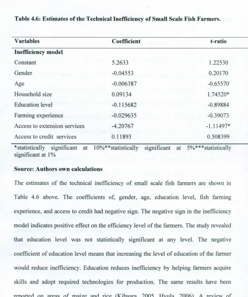
Results presented in Table 4.2 revealed that the null hypothesis was not rejected thus Cobb Douglas production function was considered to be the best represent the data. Esmeali, (2006), while estimating technical efficiency in Iranian Persian fishery similarly rejected a translog production function, while Hyuha (2006) rejected the null hypothesis. The null hypothesis was that the functional form had no inefficiency factors and the alternative had the inefficiency factors that included age, gender, household size, and level of education, fish farming experience, access to extension services, and access to credit services. The null hypothesis suggesting that the farmers were technically efficient was rejected and the alternative hypothesis that the farmers were

-,

4.3.2 Technical Efficiency of Small Scale Fish Farmers in Kiambu County

This section analyses technical efficiency of small fish farmers and presents their

efficiency levels in table 4.3 below.

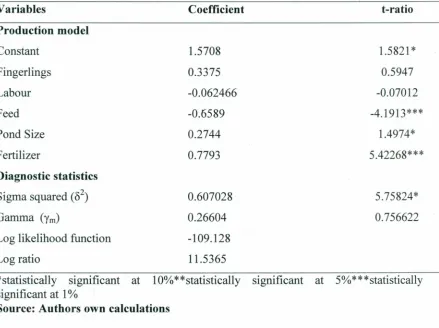
Table 4.3: Maximum Likelihood Estimates of the Stochastic Frontier Production

Function for Small Scale Farmers.

Variables Coefficient t-ratio

Production model

Constant Fingerlings Labour Feed Pond Size Fertilizer

1.5708 1.5821*

0.3375 0.5947

-0.062466 -0.07012

-0.6589 -4.1913***

0.2744 1.4974*

0.7793 5.42268***

Diagnostic statistics

Sigma squared (82)

Gamma (Ym)

Log likelihood function

Log ratio

0.607028

0.26604

-109.128

11.5365

5.75824*

0.756622

*statistically significant at 10%**statistically significant at 5%***statistically

significant at 1%

Source: Authors own calculations

Table 4.3 above shows the maximum likelihood estimates of the stochastic frontier

production function for small scale fish farmers. As shown in the Table 4.3, the

estimated sigma squared (82) of 0.607 was significantly different from zero at 10%

specified distributed assumption of the composite error term. The gamma (Ym) value

was 0.26604 though not significant at any level confirmed that farmers in the study area

were not producing along the frontier level. Gamma (Ym) is bound between zero and one

(Battese, 1992). Where it is zero, inefficiency effects do not exist in the model and if it

is one, inefficiency is significant and is not random. This means that the observed

inefficiencies are related to farmer practice.

The upper part of Table 4.3 shows the maximum likelihood estimates of the production

model. It indicates that feed consumed, pond size and fertilizer were significant at 1%,

10% and 1% respectively. However fingerlings and labour were not significant at any

level. Furthermore labour had negative coefficient. The implication of the results is that

the optimum level of labour utilization under the current scale of fish production in the

study area had been reached. This is true considering the fact that the fish ponds were

small hence may not have required a lot of manual work.

The coefficient of feed was negative and statistically significant at 10% level. This

implies that increasing the amount of feed by 10% will reduce the output of fish by the

same percentage. This result may be due to the fact that the more the farmers feed the

fish daily with low quality feed, the less their output efficiency. These findings

contradict the findings of Inoni (2007) who suggested that for fish to reach maximum

market size, quantity and quality of feed must increase, holding other inputs constant.

According to. Inoni (2007), improving the yield requires fast growing fingerlings of

coefficient of fingerlings may be attributed to the farmer's goal to realize the highest

output from the resources employed in production. The coefficient of pond size was

positive implying it affected positively the output of farmed fish. The positive and the

significance level of pond size implied direct relationship between the variable and fish

output. As the pond size increases given other inputs, fish output will increase. This is because the pond is one important variable upon which production in fish farming

depends. This finding is consistent with the findings of (Nwosu et al., 2012) who noted

that the more the size of the pond increases the farmer's output increase.

Inoni (2007) opined that if other inputs are available to expand, the farmer will have to

expand the size of his ponds if existing ponds are stocked to the maximum capacity.

Fertilizer application positively affected the output of fish in the study area. This was

shown by the positive coefficient of fertilizer and its significance level of 1%, the

implication of the result meant if fish output is to be increased fertilizer usage should be

4.3.4 Level of Technical Efficiency among the Small Scale Fish Farmers in Kiambu

County

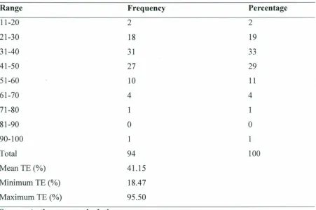
Table 4.4: Frequency Distribution of Technical Efficiency (%) in Small scale Fish

Farming.

Range Frequency Percentage

11-20 2 2

21-30 18 19

31-40 31 33

41-50 27 29

51-60 10 11

61-70 4 4

71-80 1 1

81-90 0 0

90-100 1 1

Total 94 100

Mean TE (%) 41.15

Minimum TE (%) 18.47

Maximum TE (%) 95.50

Source: Authors own calculations

The efficiency distribution Table 4.4 above shows that, efficiency of small scale fish farming is distributed across a wide range of frequency and no farmer has attained the

frontier level of a hundred percent. The result indicated that about 2% of fish farmers are operating at 70% or more technical efficiency levels. Furthermore, about 17% of

fish farmers are operating ata technical efficiency level of 50% or more. The result also

suggests that for the technical efficiency level of less than 50%, there were about 83%

The predicted farm specific technical efficiency ranged between 18.47% and 95.37%.

The average mean of the study was 41.15% which is below the frontier level. About

54% of the farmers are operating below the mean technical efficiency of 41%. This

means that in the short run, there is room for increasing fish production by about 59%

by adopting the new technology and techniques used by the best practiced fish farms.

The low levels could be related to low input usage as well as farm specific factors such

as lack of specialized extension services and education level. Capacity for improving

the existing technical efficiency level to that of the best farm in the country or fairly

different level is possible. This is by placing emphasis on farmer education and

extending targeted or specialized extension education which are considered low cost

4.3.5 Technical Efficiency Distribution and Household Characteristics

Table 4.5: Summary of technical efficiency by household characteristics.

Technical efficiency Standard

Household characteristics Mean Dev

p

Secondary 44.59 1.93

0.813

Tertiary 41.8 2.59

University 55.13 _7.39

Extension 0 42.23 4.17

0.002

1 40.58 1.2

House Hold Size 1-5 46.62 1.89

6+ 35.92 1.34 <0.001

Farming Experience 0-3 42.57 40.93

4-6 39.15 37.13

Age < 30 55.64 10.63

30-49 40.8 1.5

50-69 40.02 1.51 0.29

70+ 40.81 7.91

Credit No 41.22 1.42

Yes 40.88 2.93 1

Gender Female 41.25 2.29

Male 41.12 1.52 0.81

Table 4.5 above shows summary statistics of efficiency score by household

characteristics (age, gender, household size, and level of education, fish farming experience, access to extension services, and access to credit services). The results revealed that there was a statistically significance difference in technical efficiency

between the farmers who accessed the extension services and those who did not access .

the service as shown by the p-value of 0.002 and standard deviation of 4.17 for those

who did not and .1.2 for those who accessed. Similarly there was statistically