Reducing the Complexity of Normal Basis Multiplication
¨
Omer Eˇgecioˇglu and C¸ etin Kaya Ko¸c Department of Computer Science University of California Santa Barbara
{omer,koc}@cs.ucsb.edu
Abstract
In this paper we introduce a new transformation method and a multiplication algorithm for multiplying the elements of the field GF(2k
) expressed in a normal basis. The number of XOR gates for the proposed multiplication algorithm is fewer than that of the optimal normal basis multiplication, not taking into account the cost of forward and backward transformations. The algorithm is more suitable for applications in which tens or hundreds of field multiplications are performed before needing to transform the results back.
1
Introduction
Arithmetic operations in finite fields GF(q) have several applications in cryptography, coding, and computer algebra. Particularly of interest are fields of characteristic 2, where q = 2k, which have
various uses in elliptic curve cryptography for large values ofk, usually in the range from 160 to 521. Furthermore, smaller fields, for example, k= 8 (AES/Rijndael) and k= 2, . . . ,32 (Reed-Solomon and BCH codes) are also commonly used. Elliptic curve cryptographic protocols generally require fast hardware and software implementations of the multiplication and inversion operations. On the other hand circuits for these operations for small fields may be implemented completely in hardware and/or using a table lookup approach.
The subject of this paper is multiplication algorithms in the binary extension fields GF(2k).
There are essentially two categories of algorithms, based on the representation of field elements using polynomial basis or normal basis. In this paper, a new transformation method and a new multiplication algorithm for normal basis is introduced. First we will review the existing algorithms for both polynomial and normal bases, and then introduce the transformation method, which maps the elements of the field uniquely to the same set. This also slightly changes the definition of multiplication, as the product is computed in the transformed domain. The resulting algorithm is useful for applications where several normal basis multiplications are performed, as is the case for elliptic curve cryptography.
2
Polynomial Basis Multiplication
In the polynomial basis a field element a ∈ GF(2k) is represented as a polynomial of degree less
than or equal to k−1, written as a(x) =Pk−1
i=0 aixi with coefficients ai ∈ {0,1}. The addition of
two field elements a and b is accomplished by adding the coefficients ai and bi in GF(2), which is
first computing the degree 2k−2 product polynomialc′(x) =a(x)b(x) and then reducing it modulo
the irreducible polynomial p(x) of degree k, in order to obtain the product c(x) of degree at most
k−1:
c(x) =a(x)b(x) modp(x) .
The multiplication of the individual coefficients ai and bi require 2-input AND gates, while the
steps of the multiplication is accomplished by shift and XOR operations in software, or rewiring and XOR gates in hardware.
There are various polynomial basis multiplication algorithms; the work of Mastrovito is quite remarkable [14, 15]. This was followed up in [19, 25, 8, 28].
The properties of the irreducible polynomialp(x) are also important, and not to be overlooked. In general, low Hamming weight irreducible polynomials [23], for example, trinomials and pen-tanomials are preferred. These yield many efficient algorithms [11, 9, 27]. A comprehensive list of polynomial basis multiplication algorithms can be found in [5].
A polynomial basis multiplication algorithm of interest is the Montgomery multiplication algo-rithm, proposed by Ko¸c and Acar in [12]. This algorithm has three important properties that do not exist in the common algorithms found in the literature. The first property is that it works for general irreducible polynomials, not just special ones (such as trinomials, pentanomials, or all-one polynomials), making it more suitable for software implementations of cryptographic algorithms. The second property is that, it actually computes
¯
c(x) = MonPro(¯a(x),¯b(x)) = ¯a(x)¯b(x)x−kmodp(x), (1)
instead of the usualc(x) =a(x)b(x) modp(x). This algorithm is actually the polynomial analogue of the Montgomery multiplication algorithm for integers [16, 13]. In order to compute a field multiplication, the elementsaandbare firstforward transformedinto the polynomial Montgomery domain
a→¯a : ¯a(x) =a(x)xkmodp(x)
b→¯b : ¯b(x) =b(x)xk modp(x)
and then, the Montgomery product is computed
¯
c(x) = ¯a(x)¯b(x)x−kmodp(x)
= a(x)xkb(x)xkx−k modp(x)
= a(x)b(x)xkmodp(x) ,
which is equal to c(x)xk. When the result ¯cneeds to be transformed back to c, we use
¯
c→c : c(x) = ¯c(x)x−k modp(x) .
Of course, in order to be useful, one should not be needing too many forward c→c¯and backward ¯
c→ctransformations. This is never a problem for applications we are considering, such as elliptic curve cryptography, where tens of field multiplications are performed for each elliptic curve point addition and doubling operations, and hundreds of field multiplications are performed for elliptic curve point multiplication operations.
word-by-word, due to the properties of the Montgomery multiplication for integers [16, 13]. How-ever, it can be argued [4] that this is a moot point, since in most cases, we have low Hamming weight irreducible polynomials (trinomials and pentanomials) and there is no particular need for general irreducible polynomials.
Before closing this section we should also add that the Montgomery multiplication in GF(2k)
is not the only transformative multiplication algorithm; there are also spectral methods [21, 22], embedding techniques [24], and transformation of the field elements into polynomials [26].
3
Normal Basis Multiplication
An element β of the field GF(2k) is called a normal element, if all 2k elements of the field can be
uniquely written as a linear sum of the powers of two powers ofβ as
a =
k−1 X i=0
aiβ2
i
= a0β+a1β2+a2β4+· · ·+ak−1β2
k−1
,
such that ai ∈ {0,1}. Since the work of Kurt Wilhelm Sebastian Hensel in 1888, we know that
there always exists a normal element for any primep and integer kfor the field GF(pk).
The normal representation of a= (ak−1ak−2· · ·a1a0)∈GF(2k) is particularly useful for
squar-ing the element a. Sinceβ2k =β, we obtain a2 as
a2 = (a0β+a1β2+a2β4+· · ·+ak−1β2
k−1
)2
= a0β2+a1β4+a2β8+· · ·+ak−1β2
k
= ak−1β+a0β2+a1β4+a2β8+· · ·+ak−2β2
k−1
= (ak−2ak−3· · ·a1a0ak−1).
Therefore, the normal expression ofa2is obtained by left-rotating the digits of the normal expression ofa. The ease of squaring in normal basis is remarkable, but the multiplication is more complicated. In the following we explain the steps of the normal basis multiplication, which will be used to develop a new transformation method and normal basis multiplication algorithm.
In order to describe the computational requirements of the normal basis multiplication, we follow the steps of the Massey-Omura algorithm [18, 20], which gives the general outline for normal basis multiplication. Given the input operandsaandb, the Massey-Omura multiplier first generates all partial productsaibj for 0≤i, j≤k−1 using AND gates, and then sums these partial product
terms using multi-operand adders (whose unit element is an XOR gate).
There arek2 partial product termsaibj, a computation that can be performed usingk2 2-input
AND gates in a single AND gate delay. Decidedly this computation is optimal; k2 is both upper and lower bound on the number of partial product terms, because all of them need to be computed. However, in the computation of each of the product terms cr for 0≤r ≤k−1, we need only
a subset of the k2 partial product terms aibj. According to the optimality argument [17] of the
normal basis multiplication, the number ofaibj terms needed to compute any ofcr is at least 2k−1
for GF(2k). If there exists a normal basis for which the number ofa
ibj terms for computing any of cr is exactly 2k−1 for GF(2k), then this normal basis is called optimal. It should be noted that
optimal normal bases do not exist for every value ofk in GF(2k), which is easily verified for small
Several constructions of optimal normal bases are given in [17], together with a conjecture that describes all finite binary field extensions which have an optimal normal basis. It was proven by Gao and Lenstra in [7, 6] that the optimal normal basis constructions given in [17] are indeed all there is. These constructions are summarized in the theorem below:
Theorem 1. An optimal normal basis for GF(2k) exist only in either of the following cases:
1. If k+ 1 is prime and 2 is a primitive element inZk+1, then each of the k nonunit (k+ 1)th
root of unity forms an optimal normal basis in GF(2k).
2. If 2k+ 1 is prime and
2a: Either, 2 is primitive in Z2k+1;
2b: Or, 2k+ 1 = 3 (mod 4) and 2 generates quadratic residues in Z2k+1;
then, β = γ +γ−1 generates an optimal normal basis in GF(2k), where γ is a primitive
(2k+ 1)th root of unity.
For historical reasons, the optimal normal bases that satisfy the first part of the above theorem are named Type 1, while the ones that follow from the second part are named Type 2 bases.
3.1 Optimal Normal Multiplication in GF(22)
The elements of GF(22) expressed in polynomial basis are {0,1, x, x + 1}. There is only one irreducible polynomial of degree 2 over GF(2), which is p(x) = x2 +x+ 1. Since k+ 1 = 3 is prime, and 2 is a primitive element inZ3 (because 21 = 2 and 22 = 1), the field GF(22) has Type 1
optimal normal basis. The 2 nonunit 3rd roots of the unity in GF(22) are the two optimal normal basis elements of GF(22), and they arex and x+ 1, becausex3 = (x+ 1)3 = 1 modp(x).
We illustrate the normal basis multiplication in GF(22) using the optimal normal elementβ =x. Let the normal representations of two operands given asa=a0β+a1β2 and b=b0β+b1β2. The
productc is equal to
c=a0b0β2+a0b1β3+a1b0β3+a1b1β4 .
This expansion contains the termsβ2,β3andβ4. First we need to obtain the normal representation of β3. Since β = x, we have β2 = x2 = x+ 1 modp(x), and thus, β3 = x(x + 1) = x2 +x = 1 modp(x). Furthermore,β+β2 =x+x+ 1 = 1, and thus, we have
β0 = β+β2 = 1, β1 = β = x ,
β2 = β2 = x+ 1,
β3 = β+β2 = 1.
Substituting β3 and β4 withβ+β2 and β in the expansion of the product c, we obtain
c = a0b0β2+a0b1(β+β2) +a1b0(β+β2) +a1b1β
= (a0b1+a1b0+a1b1)β+ (a0b0+a0b1+a1b0)β2 (2)
which gives the individual terms of the productcas
c0 = a0b1+a1b0+a1b1
We now define the k×k matrix λ such that λij =β2i+2j for 0≤i, j ≤k−1, which for k= 2 is
given as
λ=
β2 β3 β3 β4
=
β2 β+β2 β+β2 β
=
0 1 1 1
β+
1 1 1 0
β2 = λ(0)β+λ(1)β2 (4)
We will explain some properties of λ in the following subsection, however, it suffices to say that
the matrix λ has k(2k−1) = 6 entries (3 in each column or 3 in each row). Furthermore, when
it is expanded into the powers of β, we obtain the 0-1 matrices λ(0) and λ(1), each of which has
2k−1 = 3 nonzero entries.
3.2 Optimal Normal Multiplication in GF(23)
We now illustrate the normal basis multiplication in GF(23), which has Type 2 optimal normal basis. We use the optimal normal elementβ =x+ 1, and irreducible polynomialp(x) =x3+x+ 1. In this section we will also describe certain properties of the λ matrices that are relevant to our
proposed multiplication algorithm. Let aand bgiven as
a = a0β+a1β2+a2β4 ,
b = b0β+b1β2+b2β4 .
The productc would be
c = a0b0β2+a0b1β3+a0b2β5+a1b0β3+a1b1β4+a1b2β6+
a2b0β5+a2b1β6+a2b2β8 . (5)
This expansion contains terms β2, β4, and β8. Since β8 =β, these are the powers of 2 powers of
β, required for normal representation in GF(23). However, the above expansion ofc also contains
other powers: β3, β5, and β6. All powers of β can be expressed in polynomial basis, reduced modulo the irreducible polynomial p(x), generating a conversion table between the powers of β
and the elements of the field represented in polynomial basis. Furthermore, once the polynomial representations ofβ,β2 and β4 are obtained, we can also obtain the normal representations of all elements. Table 1 contains the polynomial, the normal, and the powers ofβ representations of the field elements.
Table 1: The normal and the powers of β =x+ 1 representations of elements in GF(23) with irreducible polynomial p(x) =x3+x+ 1.
β4+β2+β β0
β β1
Substituting the powers of β in the expansion of the product cin Eqn. (5), we obtain
c = a0b0β2+a0b1(β+β4) +a0b2(β2+β4) +a1b0(β+β4) +a1b1β4+a1b2(β+β2) +
a2b0(β2+β4) +a2b1(β+β2) +a2b2β
= (a0b1+a1b0+a2b2+a1b2+a2b1)β+ (a0b0+a0b2+a2b0+a1b2+a2b1)β2+
(a0b1+a1b0+a0b2+a2b0+a1b1)β4 .
which gives the individual terms of the productcas
c0 = a0b1+a1b0+a2b2+a1b2+a2b1 ,
c1 = a0b0+a0b2+a2b0+a1b2+a2b1 , (6)
c1 = a0b1+a1b0+a0b2+a2b0+a1b1 .
The k×kmatrixλ with entries λij =β2i+2j for 0≤i, j≤k−1 is given as
λ=
β2 β3 β5 β3 β4 β6 β5 β6 β8 =
β2 β+β4 β2+β4 β+β4 β4 β+β2 β2+β4 β+β2 β
. (7)
Theλmatrix contains all powers ofβ needed in the computation ofc, as given in Eqn. (5). It can
also be expressed by separating the powers of β as
λ=
0 1 0 1 0 1 0 1 1
β+
1 0 1 0 0 1 1 1 0
β2+
0 1 1 1 1 0 1 0 0
β4 = λ(0)β+λ(1)β2+λ(2)β4 , (8)
where, the 3×3 matrices λ(r) forr = 0,1,2 have entries in{0,1}. Since the productc in Eqn. (5)
can be written as
c =
2 X
i=0 2 X j=0
aibjβ2
i+2j
=
2 X
i=0 2 X j=0
aibjλij
=
2 X
i=0 2 X j=0
aibjλ(0)ij β+ 2 X
i=0 2 X j=0
aibjλ(1)ij β2+ 2 X i=0
2 X j=0
aibjλ(2)ij β4
By expressing casc=c0β+c1β2+c2β4, we can write the individual terms of the productcr as
cr = 2 X
i=0 2 X j=0
aibjλ(ijr) .
The complexity of computing the terms cr depends on the number of 1s in the matrices λ(r) for r= 0,1,2. Furthermore, the matrices λ(r)
ij have the following properties:
λ(ijr) = λ(jir) (9)
λ(r+1)
i+1,j+1 = λ (r)
i,j (10)
The first property is due to the fact that 2i+ 2j = 2j + 2i, and thus,
The second property follows from the fact that 2i+1+ 2j+1 = 2(2i+ 2j), and thus
β2i+1+2j+1 = (β2)2i+2j ,
which implies
λi+1,j+1(β) =λi,j(β2) .
Considering also the fact that β2k =β, we obtain Eqn. (10). Note that all index arithmetic, i.e., increments such asi+ 1 andj+ 1 are considered mod 3 in GF(23) or mod kin GF(2k).
The optimal basis theorem [17, 7] teaches that if the normal element β is optimal, then each one of the matrices λ(r)
ij for 0 ≤ r ≤ k−1 has 2k−1 nonzero entries, as was the case for both
GF(22) in Eqn. (4) and GF(23) in Eqn. (8), where we have 2·2−1 = 3 and 2·3−1 = 5 nonzero elements in each matrix. Equivalently, the matrixλ hask(2k−1) individual terms such that each
term is a power of 2 power of β, as was shown in Eqn. (4) for GF(22) and Eqn. (7) for GF(23), which has 15 terms.
3.3 Complexity and Implementation
While there are several different ways of putting things together, the basic outline of a normal basis multiplier has 2 steps:
• Step 1: Computeaibj terms usingk2 2-input AND gates.
• Step 2: Sum the subset of the terms as implied by the nonzero entries of the λ(r)
ij matrix
using 2k−2 2-input XOR gates for each cr term.
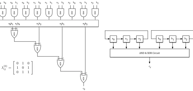
Step 1 and Step 2 can be performed sequentially, partially parallel, or fully parallel. Since Step 1 is pretty obvious, that is, it computes k2 different things, there is no need to dwell on it. Step 2, on the other hand, provides several different implementations and optimizations. For example, we can implement a single circuit consisting of 2k−2 XOR gates (arranged either as a linear array or a binary tree) to computec0, and reuse the same circuit for computingcr forr= 1,2, . . . , k−1, by
only shifting the input operandsai andbj for 0≤i, j≤k−1. Figure 1 illustrates the construction.
!" #"
AND
!" #$
AND
!" #%
AND
!$ #"
AND
!$ #$
AND
!$ #%
AND
!% #"
AND
!% #$
AND
!% #%
AND
XOR
&"
XOR
XOR
XOR
!"#$!$#" !$#% !%#$ !%#%
'()*+*,-.*/01&203
!" !$ !% #" #$ #%
&1
We are intentionally ignoring some of the details of the circuit in Figure 1, since there are various ways to arrange the circuit elements, for example, sequential, parallel, systolic, and pipelined circuits have been designed [2, 3, 1]. Our focus in this paper is not on how the individual steps of the optimal normal basis multiplications are performed or how individual circuit elements are arranged. Rather, we are interested in discovering whether there is another way to multiply two elements expressed in a normal basis defined by β in GF(2k).
4
The Proposed Method
Let aand bbe expressed in an optimal normal basis, using the normal element β in GF(2k). The
multiplication of aand bproducesc, expressed as
c=
k−1 X i=0
k−1 X j=0
aibjβ2
i+2j
=
k−1 X i=0
k−1 X j=0
aibjλij , (11)
such that the k×k matrix λ has k(2k−1) terms of type β2i fori = 1,2, . . . , k−1. Let α be a
fixed element of GF(2k),such thatα6= 0,1. We will also needα−1 which can be precomputed using
the extended Euclidean algorithm or the Fermat’s method, or the Itoh-Tsujii method [10], which is actually based on the Fermat’s method.
We define a new multiplication function, which we denote as NewPro, that takes two elements ¯
aand ¯bof the field GF(2k), which are the forward transformations of aand b, as
a→¯a : ¯a=a·α−1 , (12) b→¯b : ¯b=b·α−1 . (13)
The transformation requires the precomputedα−1 value. The operands aandbare now expressed
in “bar” domain. The NewPro algorithm takes ¯aand ¯bas input and computes ¯cas
¯
c = NewPro(¯a,¯b) = ¯a·¯b·α . (14)
After the multiplication, the resulting ¯c can be backward transformed to “nobar” domain using
¯
c→c : c = ¯c·α . (15)
since
¯
c·α= (¯a·¯b·α)·α = (a·α−1)·(b·α−1)·α2=a·b .
We call the fixed element α as the NewPro transformation constant. We apply forward transfor-mation by multiplying with α−1 and backward transformation by multiplying with α.
This new transformation method reminds us of the Montgomery transformation, however, no polynomial analogue of the Montgomery multiplication algorithm is implied here. Instead, we will propose a direct method to obtain ¯c from ¯a and ¯b, that will require fewer XOR gates than the optimal normal basis multiplication. However, this does not mean that the optimal normal basis multiplication is not optimal. The optimal normal basis multiplication computes c =a·b, while our algorithm computes ¯c= ¯a·¯b·α for a judiciously selected (and fixed) element α∈GF(2k).
Before proceeding, we should also add that both forward and backward transformations are trivially performed using the NewPro algorithm:
a→a¯ : NewPro(a, α−2) = a·α−2·α = ¯a ,
¯
a→a : NewPro(¯a,1) = (a·α−1)·1·α = a . (16)
For these computations, we need α−2, which is easily obtained from the normal representation of α−1 by a left rotation of the digits. We also need the normal representation of the unity element,
which is given as (11· · ·1) =Pk−1 i=0 β2
i
for any normal element β.
Also, if two elements are expressed in the bar domain, then their additions produce the output in the bar domain, that is
¯
a+ ¯b=a·α−1+b·α−1 = (a+b)·α−1 =c·α−1 = ¯c .
Finally we should remark that, similar to (11), the NewPro function for computing ¯c= ¯a·¯b·α can be expanded as
¯
c=
k−1 X i=0
k−1 X j=0
¯
ai¯bjλij ·α =
k−1 X i=0
k−1 X j=0
¯
ai¯bj(αλij) .
This is the usual normal basis multiplication, however, the matrix involved is αλ, instead of just λ, for a fixed element α of the field GF(2k). The matrixλ hask(2k−1) terms of type β2i, which
determines the number of 2-input XOR gates as 2k−2 for computing each component of cr for
0≤r≤k−1.
In order to have a reduced complexity (in terms of the XOR gates) normal basis multiplication, we need to show that there exists a special element α of GF(2k) for which αλ has fewer than k(2k−1) terms of type β2i. We will show the construction of α and the analyses for the fields GF(22), GF(23), and GF(24) below, and then describe the general cases.
4.1 Complexity of NewPro Multiplication in GF(22)
The proposed NewPro algorithm requires the existence of a special element αof GF(2k) such that
the matrix αλ has fewer than k(2k−1) terms of type β2i. Since GF(22) has only two suitable elements β and β2, we can easily try each one to see if the number of terms in the matrix αλ is
less than 6. First we considerα=β:
αλ=βλ=β
β2 β+β2 β+β2 β
=
β3 β2+β3 β2+β3 β2
=
β+β2 β β β2
Indeed the resulting αλ has 5 terms, instead of 6. This gives theαλ(r) matrices as
αλ=βλ=
1 1 1 0
β+
1 0 0 1
β2
We obtain the individual components of the product ¯c as
¯
c0 = ¯a0¯b0+ ¯a0¯b1+ ¯a1¯b0 ,
¯
Therefore we showed that the NewPro multiplication ¯c = NewPro(¯a,¯b) = ¯a¯bα requires only 3 2-input XOR gates using the above formulae with the selection of α =β, instead of 4 2-input XOR gates required by the normal product computationc=ab, as given by the formulae in Eqn. (3).
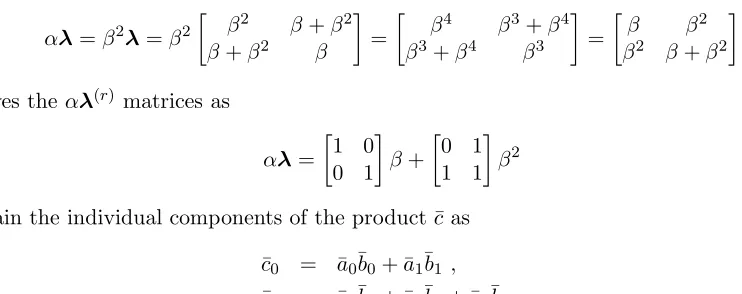
It turns out thatα =β2 also reduces the complexity:
αλ=β2λ=β2
β2 β+β2 β+β2 β
=
β4 β3+β4 β3+β4 β3
=
β β2 β2 β+β2
This gives the αλ(r) matrices as
αλ=
1 0 0 1
β+
0 1 1 1
β2
We obtain the individual components of the product ¯c as
¯
c0 = ¯a0¯b0+ ¯a1¯b1 ,
¯
c0 = ¯a0¯b1+ ¯a1¯b0+ ¯a1¯b1 .
The NewPro multiplication ¯c = NewPro(¯a,¯b) = ¯a¯bα requires only 3 2-input XOR gates using the above formulae with the selection ofα=β2, instead of 4 2-input XOR gates required by the regular normal basis multiplication c=ab, as given by the formulae in Eqn. (3).
4.2 Complexity of NewPro Multiplication in GF(23)
The proposed NewPro algorithm requires the existence of a special element αof GF(2k) such that
the matrixαλhas fewer thank(2k−1) terms of typeβ2i. For a small field such as GF(23), we can
try all possible candidates for α. Since our construction excludes α as 0 or 1, we need to try only 6 different α values in GF(23). We have performed this search using a simple Mathematica code, and obtained the number of elements in the αλ matrix for each value of α, as shown in Table 2.
Note that without the transformation, the matrix λhask(2k−1) = 15 terms.
Table 2: The number of terms in the matrix αλfor GF(23).
α Terms
β 17
β2 17
β4 17
β+β2 14
β+β4 14
β2+β4 14
The search shows that for α=β+β2, α=β+β4, and α =β2+β4 values the matrixαλhas
only 14 terms, which is 1 fewer than 15, the optimal value for the matrix λ.
We show how to obtain the αλ matrix for α =β+β2. We first multiply (β+β2) with every
term of the matrix λ, and then substitute the powers of β which are not powers of 2, using the
normal representations of all elements given in Section 3.1.
αλ= (β+β2)
β2 β+β4 β2+β4 β+β4 β4 β+β2 β2+β4 β+β2 β
=
β β2 β4
β2 β+β4 β2+β4 β4 β2+β4 β+β2+β4
As is observed, this matrix has 14 terms. We can expand this matrix in terms ofλ(r)matrices and
powers of β, to obtain
αλ=
1 0 0 0 1 0 0 0 1
β+
0 1 0 1 0 1 0 1 1
β2+
0 0 1 0 1 1 1 1 1
β4 .
Since we destroyed the shift property (Eqn. 10) of λ(r) matrices by multiplying α with λ, these
matrices no longer have the same number of 1s, however, the total number of 1s is 3 + 5 + 6 = 14, instead of 5 + 5 + 5 = 15. Finally, we obtain the individual components of the ¯c vector as
¯
c0 = ¯a0¯b0+ ¯a1¯b1+ ¯a2¯b2 ,
¯
c1 = ¯a0¯b1+ ¯a1¯b0+ ¯a1¯b2+ ¯a2¯b1+ ¯a2¯b2 ,
¯
c2 = ¯a0¯b2+ ¯a1¯b1+ ¯a1¯b2+ ¯a2¯b0+ ¯a2¯b1+ ¯a2¯b2 .
which requires 11 2-input XOR gates, instead of 12. The other two α values also produce the
λ matrices with exactly 14 terms, and the associated formulae for the components ¯cr are easily
obtained.
4.3 Complexity of NewPro Multiplication in GF(24)
Given the irreducible polynomialp(x) =x4+x+1 generating the field GF(24), we obtain an optimal normal elementβ=x3 using the construction in Theorem 1. This field has Type 1 optimal normal basis sincek+ 1 = 5 is prime, and 2 is primitive inZ5.
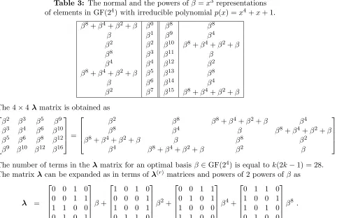
Table 3: The normal and the powers of β=x3 representations of elements in GF(24) with irreducible polynomial p(x) =x4+x+ 1.
β8+β4+β2+β β0 β8 β8
β β1 β9 β4
β2 β2 β10 β8+β4+β2+β
β8 β3 β11 β
β4 β4 β12 β2
β8+β4+β2+β β5 β13 β8
β β6 β14 β4
β2 β7 β15 β8+β4+β2+β
The 4×4λ matrix is obtained as
β2 β3 β5 β9 β3 β4 β6 β10 β5 β6 β8 β12 β9 β10 β12 β16 =
β2 β8 β8+β4+β2+β β4
β8 β4 β β8+β4+β2+β
β8+β4+β2+β β β8 β2
β4 β8+β4+β2+β β2 β
The number of terms in the λmatrix for an optimal basis β ∈GF(24) is equal tok(2k−1) = 28.
The matrix λcan be expanded as in terms of λ(r) matrices and powers of 2 powers of β as
λ =
0 0 1 0 0 0 1 1 1 1 0 0 0 1 0 1
β+
1 0 1 0 0 0 0 1 1 0 0 1 0 1 1 0
β2+
0 0 1 1 0 1 0 1 1 0 0 0 1 1 0 0
β4+
0 1 1 0 1 0 0 1 1 0 1 0 0 1 0 0
The total number of 1s in these matrices is also 28, each of which has 7 1s. Therefore, we need 6 2-input XOR gates to computes each one of thecr terms forr = 0,1,2,3, which totals to 24 XOR
gates. Similar to the case GF(23), we performed an exhaustive search over the set GF(24) and obtained the list of αvalues, and the minimum number of terms in the matrix αλ, as summarized
in Table 4.
Table 4: The minimum number of terms in the matrixαλfor GF(24).
α Terms
β 25
β2 25
β4 25
β8 25
It turns out that there are only 4 α values, which minimize the number of terms in the matrix
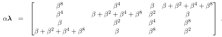
αλ; the minimum value is found as 25. We obtain the matrix αλ forα=β, by multiplying every
element of the matrix byα. The elements of the matrix which contains the powers ofβ which are not powers of 2 are then replaced with their normal expansions.
αλ =
β8 β4 β β+β2+β4+β8 β4 β+β2+β4+β8 β2 β
β β2 β4 β8
β+β2+β4+β8 β β8 β2
.
The matrixαλhas exactly 25 terms. It can be expanded in terms of λ(r) matrices and powers of
2 powers of β as
αλ =
0 0 1 1 0 1 0 1 1 0 0 0 1 1 0 0
β+
0 0 0 1 0 1 1 0 0 1 0 0 1 0 0 1
β2+
0 1 0 1 1 1 0 0 0 0 1 0 1 0 0 0
β4+
1 0 0 1 0 1 0 0 0 0 0 1 1 0 1 0
β8 .
The total number of 1s in these matrices is also equal to 25. The number of 2-input XOR gates to compute ¯cr terms forr = 0,1,2,3 is found as 6 + 5 + 5 + 5 = 21.
5
The General Case for GF
(2
k)
The NewPro transformation and the multiplication algorithms require the existence of an element
α of GF(2k), that minimizes the number of terms in the αλ matrix. We gave detailed analyses
of the NewPro multiplication for the fields GF(22), GF(23) and GF(24) together with all special α values. It turns out that the number of terms in the αλ matrix are equal to 5, 14 and 25 for
GF(22), GF(23) and GF(24) respectively, while the original λmatrices have 6, 15 and 28 terms.
However, we need a more detailed analysis of the proposed NewPro algorithm, specifically, we identify the following types of problems to study:
1. Due to the optimal normal basis theorem, we know that λ hask(2k−1) terms for GF(2k).
2. Does there exist anα for any ksuch that number of terms inαλis less than k(2k−1)?
3. Is there a constructive or non-exhaustive method for finding α that reduces the number of terms to fewer thank(2k−1)?
The answers to these questions for Type 2 optimal normal bases seem to be negative fork >3. For such normal bases, no α can bring down the number of terms in αλ to a quantity below
k(2k−1). However, we settle the above questions for Type 1 optimal normal bases in the following fashion.
6
Optimality for the Type 1 Case
Let us assume that GF(2k) has a Type 1 optimal normal basis; this implies thatk+ 1 is prime and
2 is primitive in Zk+1. Moreover, the optimal normal element β is a primitive (k+ 1)st root of 1
in GF(2k). For the brevity of the notation, we writek+ 1 = 2m+ 1, β i =β2
i
, and 1 stands for the unity element in normal basis:
1=β+β2+β4+· · ·+β2k−1
=β0+β1+β2+· · ·+βk−1 .
We also use B to represent the basis set B={β0, β1, . . . , βk−1}. As before, the k×kmatrix λ is
defined as
λij =β2i+2j =βiβj
for 0≤i, j≤k−1. For example, fork= 4, we have
λ=
β1 β3 1 β2 β3 β2 β0 1
1 β0 β3 β1 β2 1 β1 β0
.
Lemma 1. The elements in the entries (0, m),(1, m+ 1), . . . ,(k−1, m+k−1) of λ, where the
indices are computed mod k, are all 1s.
Proof. What we need to show is βiβm+i = 1 for 0 ≤ i≤ k−1, where the indices are computed
mod k. Letθi=βiβm+i, and put θ=θ0 =β0βm. Then
θi=β2
i+2m+i
= β2m+12
i
=θ2i .
Therefore it suffices to show thatθ=1. Calculating,
θ2m=β2mβ22m =βmβ0 =θ ,
so thatθ2m−1=1. On the other hand,θ is a power ofβ and β2m+1 =1, soθ2m+1 =1. Therefore
the order of θ dividesd= gcd(2m−1,2m+ 1). Since p= 2m+ 1 is prime,dis either 1 or p. But
2m−1 = 2p−1
2 −1 and this cannot be divisible by p for otherwise 2 is a quadratic residue modulo p and so cannot be primitive. Therefore,d= 1 andθ=1.
The entryβiβm+i =β0+β1+· · ·+βk−1 contributeskto the sum of the number of basis vectors
appearing in row i. Since the basis is optimal, the total number of these is 2k−1. Each of the remaining k−1 entries is a single βj. By optimality, the elements in row i excluding the unit in
columnm+iis a permutation ofβ0, . . . , βi−1, βi+1, . . . , βk−1. We record the fact that the elements
Lemma 2. For an optimal normal basis of Type 1 with k+ 1 = 2m+ 1, generated by β =β0, the
row r for 0≤r ≤k−1 of λ is a permutation of B − {βr} with 1 appearing in the column index m+r modulo k. Therefore βr· {β0, β1, . . . , βk−1}=B − {βr} .
Next, we consider the matrix βrλ.
Lemma 3. Row m+r of βrλ is a permutation of B. Each of the other rows is a permutation of
B minus some basis element.
Proof. We will give the proof for r= 0. Note that every row inλ has a 1 (the entries in positions
(0, m),(1, m+ 1), . . . ,(k−1, m+k−1) are 1s), so inβλ, β0 appears in each row. By Lemma 2,
therth row of λis a permutation of B − {βr}. Therefore the rth row of βλis
1. a permutation of B − {1} forr=m,
2. a permutation of B − {β0βr}forr 6=m (note: β0βr =βj for somej in this case).
Therefore, we conclude that the total number of basis vectors appearing in the matrix is
k+ (k−1)(2k−1) =k(2k−1)−(k−1),
which is k−1 fewer than that of the multiplication matrixλ. We state the following theorem for
the Type 1 case, but omit its proof.
Theorem 2. Suppose α hast nonzero coefficients in its normal basis expansion. Then the number of terms in the matrix αλ is k(2k−1) + (k−t) (t(2k−2)−(2k−1)). In particular α = βi for
0 ≤ i≤k−1 are the only αs with the property that αλ matrix has smaller than k(2k−1), i.e.,
k(2k−1)−(k−1) basis vectors.
7
Further Work
By slightly changing the definition of the multiplication operation, we introduced a new normal basis multiplication algorithm which requires fewer XORs than the optimal normal multiplication algorithm. We proved for the Type 1 case that the number of terms in the αλ isk−1 fewer than that of λmatrix for α=βi for some 0≤i≤k−1. Appendix A gives the λand αλ matrices for
GF(2k) for k= 2,4,10,12, which are the first 4 fields that has Type 1 optimal normal bases.
Moreover, experimentation shows that the field GF(23) and Type 2 optimal normal basis matrix
αλ has 14 terms forα=β+β2,α=β+β4, andα =β2+β4 instead of 15 terms, which is clearly
unlike the Type 1 case, i.e., it is not k−1 = 2 fewer than k(2k−1) = 15. However the case of GF(23) seems to be an anomaly, and it appears that for a Type 2 optimal normal basis GF(2k) for k >3, there is noα value which gives smaller than k(2k−1) terms in αλ.
It is also possible to view αλ as matrix multiplication by αI, so one can study the suitability
References
[1] G. B. Agnew, T. Beth, R. C. Mullin, and S. A. Vanstone. Arithmetic operations in GF(2m).
Journal of Cryptology, 6(1):3–13, 1993.
[2] G. B. Agnew, R. C. Mullin, I. Onyszchuk, and S. A. Vanstone. An implementation for a fast public-key cryptosystem. Journal of Cryptology, 3(2):63–79, 1991.
[3] G. B. Agnew, R. C. Mullin, and S. A. Vanstone. An implementation of elliptic curve cryp-tosystems over F2155. IEEE Journal on Selected Areas in Communications, 11(5):804–813,
June 1993.
[4] I. Blake, G. Seroussi, and N. Smart. Elliptic Curves in Cryptography. Cambridge University Press, 1999.
[5] S. S. Erdem, T. Yanık, and C¸ . K. Ko¸c. Polynomial basis multiplication in GF(2m). Acta
Applicandae Mathematicae, 93(1-3):33–55, September 2006.
[6] S. Gao. Normal Bases over Finite Fields. PhD thesis, University of Waterloo, 1993.
[7] S. Gao and H. W. Lenstra, Jr. Optimal normal bases. Designs, Codes and Cryptography, 2(4):315–323, December 1992.
[8] A. Halbutoˇgulları and C¸ . K. Ko¸c. Mastrovito multiplier for general irreducible polynomials. IEEE Transactions on Computers, 49(5):503–518, May 2000.
[9] M. A. Hasan, M. Z. Wang, and V. K. Bhargava. Modular construction of low complexity parallel multipliers for a class of finite fields GF(2m). IEEE Transactions on Computers,
41(8):962–971, August 1992.
[10] T. Itoh and S. Tsujii. A fast algorithm for computing multiplicative inverses inGF(2m) using
normal bases. Information and Computation, 78(3):171–177, September 1988.
[11] T. Itoh and S. Tsujii. Structure of parallel multipliers for a class of finite fields GF(2m).
Information and Computation, 83:21–40, 1989.
[12] C¸ . K. Ko¸c and T. Acar. Montgomery multiplication in GF(2k). Designs, Codes and
Cryptog-raphy, 14(1):57–69, April 1998.
[13] C¸ . K. Ko¸c, T. Acar, and B. S. Kaliski Jr. Analyzing and comparing Montgomery multiplication algorithms. IEEE Micro, 16(3):26–33, June 1996.
[14] E. D. Mastrovito. VLSI architectures for multiplication over finite field GF(2m). In T. Mora,
editor, Applied Algebra, Algebraic Algorithms and Error-Correcting Codes, pages 297–309. Springer, LNCS Nr. 357, 1988.
[15] E. D. Mastrovito. VLSI Architectures for Computation in Galois Fields. PhD thesis, Link¨oping University, Department of Electrical Engineering, Link¨oping, Sweden, 1991.
[17] R. Mullin, I. Onyszchuk, S. Vanstone, and R. Wilson. Optimal normal bases in GF(pn).
Discrete Applied Mathematics, 22:149–161, 1988.
[18] J. Omura and J. Massey. Computational method and apparatus for finite field arithmetic, May 1986. U.S. Patent Number 4,587,627.
[19] C. Paar. A new architecture for a paralel finite field multiplier with low complexity based on composite fields. IEEE Transactions on Computers, 45(7):856–861, July 1996.
[20] A. Reyhani-Masoleh and M. A. Hasan. A new construction of Massey-Omura parallel multiplier over GF(2m). IEEE Transactions on Computers, 51(5):511–520, May 2001.
[21] G. Saldamlı. Spectral Modular Arithmetic. PhD thesis, Oregon State University, 2005.
[22] G. Saldamlı, Y.-J. Baek, and C¸ . K. Ko¸c. Spectral modular arithmetic for binary extension fields. InThe 2011 International Conference on Information and Computer Networks (ICICN), pages 323–328, 2011.
[23] G. Seroussi. Table of low-weight binary irreducible polynomials, August 1998. Hewlett-Packard, HPL-98-135.
[24] J. H. Silverman. Fast multiplication in finite fields GF(2n). In C¸ . K. Ko¸c and C. Paar, editors,
Cryptographic Hardware and Embedded Systems - CHES 1999, pages 122–134. Springer, LNCS Nr. 1965, 1999.
[25] B. Sunar and C¸ . K. Ko¸c. Mastrovito multiplier for all trinomials. IEEE Transactions on Computers, 48(5):522–527, May 1999.
[26] J. von zur Gathen, A. Shokrollahi, and J. Shokrollahi. Efficient multiplication using type 2 optimal normal bases. In C. Carlet and B. Sunar, editors,Arithmetic of Finite Fields, WAIFI 2007, pages 55–68. Springer, LNCS Nr. 4547, 2005.
[27] H. Wu and M. A. Hasan. Low complexity bit-parallel multipliers for a class of finite fields. IEEE Transactions on Computers, 47(8):883–887, August 1998.
Appendix A: The Type 1
λ
and
α
λ
Matrices
The λ and αλ Matrices for GF(22)
The irreducible polynomial isx2
+x+ 1. The optimal normal element isβ=x. The total count of 1s inλ andαλmatrices are 6 and 5, respectively.
λ=
"
β1 β0 β0 β1
#
, β0λ=
"
1 β0 β0 β1
#
, β1λ=
"
β0 β1 β1 1
#
The λ and αλ Matrices for GF(24)
The irreducible polynomial isx4
+x3
+ 1. The optimal normal element isβ =x+ 1. The total count of 1s inλand αλmatrices are 28 and 25, respectively.
λ=
β1 β3 1 β2 β3 β2 β0 1
1 β0 β3 β1
β2 1 β1 β0
, β0λ=
β3 β2 β0 1
β2 1 β1 β0 β0 β1 β2 β3
1 β0 β3 β1
, β1λ=
β2 1 β1 β0
1 β0 β3 β1
β1 β3 1 β2 β0 β1 β2 β3
β2λ=
β0 β1 β2 β3 β1 β3 1 β2 β2 1 β1 β0 β3 β2 β0 1
, β3λ=
1 β0 β3 β1
β0 β1 β2 β3 β3 β2 β0 1
β1 β3 1 β2
The λ and αλ Matrices for GF(210)
The irreducible polynomial isx10
+x7
+ 1. The optimal normal element isβ=x6
+x3
+x2
+x. The total count of 1s inλandαλ matrices are 190 and 181, respectively.
λ=
β1 β8 β4 β6 β9 1 β5 β3 β2 β7 β8 β2 β9 β5 β7 β0 1 β6 β4 β3 β4 β9 β3 β0 β6 β8 β1 1 β7 β5 β6 β5 β0 β4 β1 β7 β9 β2 1 β8 β9 β7 β6 β1 β5 β2 β8 β0 β3 1 1 β0 β8 β7 β2 β6 β3 β9 β1 β4 β5 1 β1 β9 β8 β3 β7 β4 β0 β2 β3 β6 1 β2 β0 β9 β4 β8 β5 β1 β2 β4 β7 1 β3 β1 β0 β5 β9 β6 β7 β3 β5 β8 1 β4 β2 β1 β6 β0
, βλ=
β8 β2 β9 β5 β7 β0 1 β6 β4 β3 β2 β4 β7 1 β3 β1 β0 β5 β9 β6 β9 β7 β6 β1 β5 β2 β8 β0 β3 1
β5 1 β1 β9 β8 β3 β7 β4 β0 β2 β7 β3 β5 β8 1 β4 β2 β1 β6 β0 β0 β1 β2 β3 β4 β5 β6 β7 β8 β9
1 β0 β8 β7 β2 β6 β3 β9 β1 β4
β6 β5 β0 β4 β1 β7 β9 β2 1 β8 β4 β9 β3 β0 β6 β8 β1 1 β7 β5 β3 β6 1 β2 β0 β9 β4 β8 β5 β1
The λ and αλ Matrices for GF(212)
The irreducible polynomial isx12
+x10
+x2
+x+1. The optimal normal element isβ=x11
+x7
+x3
+x2
+x. The total count of 1s inλandαλmatrices are 276 and 265, respectively.
λ=
β1 β4 β9 β8 β2 β11 1 β6 β10 β5 β7 β3 β4 β2 β5 β10 β9 β3 β0 1 β7 β11 β6 β8 β9 β5 β3 β6 β11 β10 β4 β1 1 β8 β0 β7 β8 β10 β6 β4 β7 β0 β11 β5 β2 1 β9 β1 β2 β9 β11 β7 β5 β8 β1 β0 β6 β3 1 β10 β11 β3 β10 β0 β8 β6 β9 β2 β1 β7 β4 1
1 β0 β4 β11 β1 β9 β7 β10 β3 β2 β8 β5
β6 1 β1 β5 β0 β2 β10 β8 β11 β4 β3 β9 β10 β7 1 β2 β6 β1 β3 β11 β9 β0 β5 β4 β5 β11 β8 1 β3 β7 β2 β4 β0 β10 β1 β6 β7 β6 β0 β9 1 β4 β8 β3 β5 β1 β11 β2 β3 β8 β7 β1 β10 1 β5 β9 β4 β6 β2 β0
βλ=
β4 β2 β5 β10 β9 β3 β0 1 β7 β11 β6 β8 β2 β9 β11 β7 β5 β8 β1 β0 β6 β3 1 β10 β5 β11 β8 1 β3 β7 β2 β4 β0 β10 β1 β6 β10 β7 1 β2 β6 β1 β3 β11 β9 β0 β5 β4 β9 β5 β3 β6 β11 β10 β4 β1 1 β8 β0 β7 β3 β8 β7 β1 β10 1 β5 β9 β4 β6 β2 β0 β0 β1 β2 β3 β4 β5 β6 β7 β8 β9 β10 β11
1 β0 β4 β11 β1 β9 β7 β10 β3 β2 β8 β5
β7 β6 β0 β9 1 β4 β8 β3 β5 β1 β11 β2 β11 β3 β10 β0 β8 β6 β9 β2 β1 β7 β4 1 β6 1 β1 β5 β0 β2 β10 β8 β11 β4 β3 β9 β8 β10 β6 β4 β7 β0 β11 β5 β2 1 β9 β1