A Data Placing Policy Established on Genetic
Algorithm in Cloud Computing
Y.Neeraja1, G.Divya Zion2, U.Supriya3 1
M.Tech(CS) Student, Ravindra College of Engineering For Women, Kurnool, A.P, India.
2
Assistant Professor, Dept of CSE, Ravindra Engineering College for Women, Kurnool, AP, India.
3
Assistant Professor, Dept of CSE, G.Pullaiah College of Engineering & Technology,
Kurnool, AP, India
Abstract
Cloud computing has become a new platform for personal computing. Cloud computing provides high performance computing resources and mass storage resources. Cloud providers use the distributed cloud computing for the better cloud services. This means that we can minimize the data scheduling between the data centers. The use of genetic algorithms to address the data placement problems in cloud computing. The experimental results show that genetic algorithm can effectively work out the approximate optimal data placement, and minimize the data scheduling between data centers.
Keywords
Cloud computing, Data placement, Genetic algorithm
I. INTRODUCTION
Cloud computing, as well on-demand computing[1], is a kind of Internet-based computing that provides community dealing out property and information to computers and other devices on demand. It is a model for enable all over the place, on-demand right to use to a shared collection of configurable computing assets. Cloud computing and storage solutions make available users and enterprise with various capabilities to store and process their data in third-party data centers. It relies on sharing of resources to achieve consistency and economy of scale, similar to a utility (like the electrical energy grid over a network). Cloud providers naturally use a "pay as you go" model. The current accessibility of high-capacity networks, not costly computers and storage space devices as well as the acknowledged acceptance of hardware virtualization, service-oriented devise and autonomic and utility computing have led to a growth in cloud computing.
Deciding how to assign data items to nodes in a distributed system in such way that they can be later retrieved [2]. It encompasses all data movement related activities such as transfer, staging, replication, space allocation and
has become huge problem. In data intensive computing if multiple computations are jointly process multiple datasets in frequent way, these data sets are supposed to be correlative with each other. The objective of data scheduling is partly to ensure that most important data are sent first, partly to ensure that any transmission is cost efficient. The data scheduling applies to data sent between the mobile host and the GSM.
II. RELATED WORK:
The promise of data-driven decision-making is now being recognized broadly, and there is growing enthusiasm for the notion of "Big Data," including the recent announcement from the White House about new funding initiatives across different agencies, that target research for Big Data. While the promise of Big Data is real -- for example, it is estimated that Google alone contributed 54 billion dollars to the US economy in 2009 -- there is no clear consensus on what is Big Data [8]. In fact, there have been many controversial statements about Big Data, such as "Size is the only thing that matters." In this panel we will try to explore the controversies and debunk the myths surrounding Big Data.
A Data Placement Strategy for Data-Intensive Applications in Cloud. With the development of information technology, data-intensive applications in cloud have been used in more and more fields. Because of the decentralized data centers in cloud, these applications now are facing some new challenges in data placement which mainly include how to reduce the time cost of data movements between data centers, how to deal with the data dependencies, and how to keep a relative load balancing of data centers. This paper proposes a data placement strategy [9], the three stages of which address the three challenges above respectively. Simulation shows that the strategy can effectively reduce the time cost of data movements across data centers during the application’s execution.
A, a data manager must intelligently select
data centers in which these data will
reside. This is, however, not the case for
data which must have a fixed location.
Placement Strategy in Scientific Cloud
Workflows, In scientific cloud workflows,
large amounts of application data need to
be stored in distributed data centers. To
effectively store these when one task needs
several datasets located in different data
centers, the movement of large volumes of
data becomes a challenge [10]. In this
paper
, we propose a matrix based k-meansclustering strategy for data placement in scientific cloud workflows. The strategy contains two algorithms that group the existing datasets in k data
centers during the workflow build-time stage, and dynamically clusters newly generated datasets to the most appropriate data centers–based on dependencies–during the runtime stage.
A Framework for Reliable and Efficient Data Placement in Distributed Computing Systems. Data placement is an essential part of today's distributed applications since moving the data close to the application has many benefits. The increasing data requirements of both scientific and commercial applications and collaborative access to these data make it even more important [11]. In the current approach, data placement is regarded as a side affect of computation. Our goal is to make data placement a first class citizen in distributed computing systems just like the computational jobs. They will be queued, scheduled, monitored, managed, and even check pointed. Since data placement jobs have different characteristics than computational jobs, they cannot be treated in the exact same way as computational jobs. For this purpose, we are proposing a framework which can be considered as a “data placement subsystem” for distributed computing systems, similar to the I/O subsystem in operating systems. This framework includes a specialized scheduler for data placement, a high level planner aware of data placement jobs, a resource broker/policy enforcer and some optimization tools. Our system can perform reliable and efficient data placement, it can recover from all kinds of failures without any human intervention, and it can dynamically adapt to the environment at the execution time.
III. SYSTEM DESIGN
In cloud computing the data storage typically achieves large amounts of data such as petabytes magnitude scale, high requirements of data service types are high level great pressure to manage the data [12]. Cloud systems have the characteristics of data-intensive and compute intensive and the concurrent execution of large scale computations in the system
A) Data scheduling between data centers in
cloud computing:
physical model of data scheduling between data center is showed in Figure 1.
Assuming that the collection of datasets stored in a distributed cloud computing system is:
D= {d1, d2, d3,……..,dn}
Where n is the number of datasets and the size of dataset di is i , i = 1, 2,….., n .
The l data centers in the system are denoted as:
S= {S1, S2, S3,……..,Sl}
The basic capacity of data center Sk.The m
computations in the system are denoted as:
C= {c1, c2, c3,……….,cm}
The execution frequencies of each computation is
U= {µ1, µ2, µ3,……, µm}
Where µ1 is the execution frequency of
computation ci in unit interval. Now we can define
a processing factor αij. The processing factor
consists of dataset dj is needed to process during
the execution of computation ci or not.
αij = 1 data set dj is needed to process ci 0 data set dj is not needed to process ci
And we can form a Association matrix for the computation set C and dataset D is denoted as A= [αij]m*n
Data placement is to distribute datasets into each data center. In this paper, data replica is out of consideration. Similarly, we define a placement factor βjk .The placement factor consists of dataset
dj is placed in datacenter Sk or not.
1 When dataset dj is placed
βjk = in data center Sk
0 When dataset dj is not placed
in data center Sk
And we can form a Association matrix for the dataset D and datacenter S is denoted as
B= [βjk] n*l
Matrix B reflects the status of the datasets D stored in the data centers S. Why because the datasets and datacenters are placed in the placement matrix i.e; matrix B. We can easily find that the sum of the elements of each row in matrix B is 1
Σl
k=1 βik=1
The sum of the elements of the kth column in
matrix B is the number of datasets stored in the data center Sk, when we place datasets into data center Sk, the stored data size should not exceed the
basic capacity of Sk, thus
Σn
j=1 βjk* j ≤ Sk
Where j is the size of the dataset and Sk is the
basic capacity of datacenter.
To place the processing matrix and placement matrix in another matrix i.e. matrix Z.
Matrix Z=A*B
This means that we can multiply the computations, datasets and datacenter. Then we can obtain the number of computations can accessing the number of datacenters.
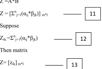
Then matrix Z as follows
Z =A*B
Z = [Σnj=1(αij*βjk)] m*l
Suppose
Zik =Σnj=1(αij*βjk)
Then matrix
Z= [zik] m*l
Where zik is the number of datasets processed when
the computation ci is performed one time in data
center. This means that the computation ci is
accessed from the datacenter Sk. The sum of
elements in each row in matrix Z, denoted as Σl k=1
zik , is the total number of times of accessing all
data centers during the execution of the computation ci , also is the number of datasets
processed during the execution of the computation
ci .
Fig 1: A physical model of data scheduling between data centers
1
2
3
4
5
6
7
8
9
10
11
12
The sum of elements in each column, denoted as
Σm
i=1 zik is the number of the datasets processed in
data center Sk when all the computations are
performed one time.
Define a u (zik) function denoted as,
u(zik ) = 1 zik≠0
0 zik=0
Then the number of data centers accessed during the execution of computation ci is
Σl
k=1 u (zik)
The number of data scheduling is (Σl
k=1 u (zik
)-1) when computation ci is executed one time.
Which means that computation ci is accessed one
time from the datacenter Sk.
When the placement matrix is B, the total number of data scheduling during the execution of all computations in the system in unit interval can be expressed as:
Γ (B) = [Σm
i=1Σlk=1u (zik)-1]*µi
Our objective is to find the optimal data placement solution B* that minimize Γ (B) . When placing datasets to data centers, we should meet the requirements of data center capacity and no duplication of data placement.
B*=
argmin{Γ(B)}
This Γ (B) requires more data scheduling. So we can reduce the data scheduling between data centers by using Genetic Algorithm.
IV. GENETIC ALGORITHM IN DATA PLACEMENT
STRATEGY
Genetic algorithm is a search method that mimics the process of natural selection. Genetic algorithm used to generate useful solutions to optimization and search problems. A solution generated by a genetic algorithm is called a chromosome. The collection of chromosomes is referred as population. These chromosomes will undergo a process called fitness function. Actually there are lots of traditional optimization algorithms such as Exhaustive search algorithm, Monte Carlo algorithm, Genetic algorithm and so on.
Exhaustive search algorithm is a randomization technique [13]. It can be used to reduce the search space. Exhaustive search algorithms are backtracking algorithms, but all backtracking algorithms are not exhaustive. These algorithms will take high computational complexity which is
approximately (ln). The exhaustive search
algorithm is possible when datasets are small.
Monte Carlo algorithm is a randomized method [14]. It uses randomness and statistics to get the result. The computation complexity has improved while compare to the Exhaustive search algorithm but the search complexity is not still high. So we can use the Genetic algorithm.
Genetic algorithm is direct method to evaluate an optimization solutions based on the natural selection and natural genetics [15]-[16]. A population consists of collection of chromosomes or individuals. For these individuals we can evaluate the fitness value, if the highest fitness value is selected from the current population, then crossover and mutation operations are performed. The best candidate solutions (individuals) are used in the algorithm for the next generation. For the best solutions we have to follow some steps.
A. Encodng:
Encoding is the way to represent the solution. In genetic algorithm the placements of datasets in datacenters is represented by matrix B. In this algorithm the matrix B is directly manipulated as a genotype.
B. Chromosome and Population
Chromosome is a set of parameters which define a proposed solution to the problem that the genetic algorithm is trying to solution. The set of all solutions is known as the population.
A population consists of several individuals and it is a subset of whole searching space.
C. Fitness Function
Fitness function is used as to summarize the solution as a single point [17]-[18]. The fitness function is a reciprocal of the objective function. In genetic algorithm the objective function is denoted as Γ (B). And fitness function (F) is F=1/ Γ (B).
A. Genetic operators
Genetic operators are used to guide the algorithm towards a solution in a given problem. In genetic algorithm we have to use 3 different types of operators.
1. Selection:
In selection process many types of selection processes. They are Roulettewheel selection, Rank selection, Steady state selection, Tournament selection. In this paper we areusing Roulettewheel selection. Why because all the chromosomes are 14
15
placed in the population, if the high fitness values are selected more times. If the fitness value is low that chromosome will be rejected.
If the selection process may follow as below.
1. The fitness function is evaluated for each individual, providing fitness values, which are then normalized. Normalization means dividing the fitness value of each individual by the sum of all fitness values, so that the sum of all resulting fitness values equals 1.
2. The population is sorted by descending fitness values.
3. Accumulated normalized fitness values are computed (the accumulated fitness value of an individual is the sum of its own fitness value plus the fitness values of all the previous individuals). The accumulated fitness of the last individual should be 1 (otherwise something went wrong in the normalization step).
4. A random number R between 0 and 1 is chosen.
5. The selected individual is the first one whose accumulated normalized value is greater than R.
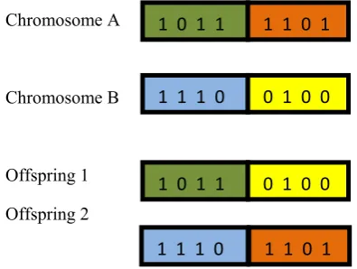
2. Crossover
Crossover is a genetic operator which can be used to vary the chromosome or chromosomes from one generation to the next.
Chromosome A
Chromosome B
Offspring 1
Offspring 2
Fig 2: A two point crossover Example 3. Mutation
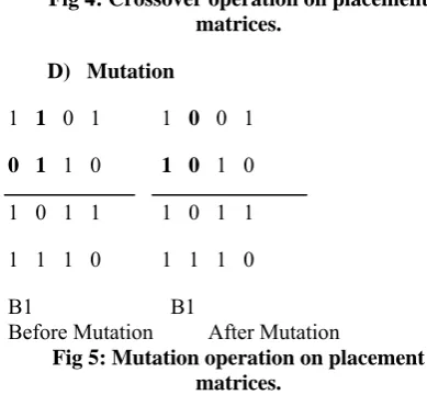
Mutation is a genetic operator, which is used to maintain genetic diversity from one generation of the chromosomes to the next. In mutation operator the selected bits are inverted, which means that 0 as 1 and vice versa.
Fig: Before Mutation
Fig: After Mutation
Fig 3: Mutation Example
V. DATA PLACEMENT STRATEGY IN GENETIC
ALGORITHM EXAMPLE
We have to place the data placement strategy in genetic algorithm following some steps.
Step 1: Determine the size of the population (L), crossover rate (Cr) and mutation rate (Mr).
Step 2: Generate initial population in random BL
(0) consists of L placement matrices. All the elements of B matrix is set to zero, then generate n different random numbers i.e; {r1, r2,…,ri,….,rn}
(0≤ri≤1).
If ri indicates that the dataset di is to be placed into
the datacenter Sri then placement matrix is changed
to 1. If the generated matrix does not meet requirements,(do not cross the limited capacity of datacenter), then it abandon and generate a new matrix.
Step 3: Calculate the each individual in the
population BL (T), T=0, 1, 2, 3,…, and generate a matrix Z by matrix multiplication, Z=A*B. the number of data scheduling is calculated from the equation(15).
Step 4: Calculate the number of data scheduling is
Γ (Bt). For each individual in each population BL
(T). The fitness value of Bt is denoted as F=1/ Γ
(Bt ).
After calculating the fitness value of each individual in population, then calculate the probabilities of L individual from BL (T) by using the roulette wheel selection.
Step 5: perform crossover operation on selected
placement matrices. The crossover rate (Cr)
indicates that percentage of chromosomes taking part in the crossover operation.
Step 6: perform mutation operation on crossover
resultants.
We have to take practical example on process of data placement based on genetic algorithm.
A Data Placement Strategy Based on Genetic Algorithm in Cloud Computing, we can minimize the data scheduling between data centers. Let us 1 0 1 1 1 1 0 1
1 1 1 0 0 1 0 0
1 0 1 1 0 1 0 0
1 1 1 0 1 1 0 1
1 1 0 1 0 1 0 1
examine the practical example on data placement strategy based on Genetic Algorithm.
Let us assume data centers as (l), datasets as (n) and computations as(c). In this example we can define Processing factor (αij) and Placement factor
(βjk).
The Association matrix (processing factor) for computation set C and Datasets D is denoted as A.
A= [αij]m*n
A=
The Association matrix (placement factor) for dataset D and datacenter S is denoted as B.
B= [βjk]n*l
B1=
Where we can define a matrix Z=A*B1
Z=[Σnj=1(αij*βjk)]m*l
Zik= *
Zik=
In the resultant matrix Z, row can be represented as data centers. And columns represented as computations. Where Σi=1m u (Zik). is the number of
the datasets processed in data center Sk when
all
the computations are performed one time.
Σi=1m u (Zik) = 5+5+6
= 11 Where Σl
k=1 u (Zik) is the total number of times of
accessing all data centers during the execution of the computation ci , also is the number of datasets
processed during the execution of the computation ci.
Σl
k=1 u (Zik) = 4+5+5+2
= 16
In this example all computations are executed one time is 16. And we can define a execution frequencies of each computation ci is denoted as µi.
The number of data scheduling is (Σlk=1 u(zik)-1)
when computation ci is executed one time.
The number of data scheduling is
(16-1) =15 when computation c1 is executed one
time.
(16-2) = 14 when computation c1 is executed
second time.
All computations are executed in the unit interval is
Γ (B= Σm
i=1 [Σlk=1 u (zik)-1]*µi
=Σm
i=1 [15*1]
Where µ1=1
Γ (B1) = [15+28+26+36+11+20+9+8+14+24+5]
=196
All computations are executed in the unit interval is 196.
In this example the processing factor is constant, and placement factor is varies. This means that
A=
B2=
Z= *
Zik=
0 1 0 1
0 1 0 1
1 0 1 0 0 1 0 1
0 1 0 1
1 0 1 0
1 1 0 1
0 1 1 0
1 0 1 1
1 1 1 0
1 1 0 1
0 1 1 0
1 0 1 1
1 1 1 0 0 1 0 1
0 1 0 1
1 0 1 0
1 2 2 0
1 2 2 0
2 1 1 2
1 1 0 1
1 1 1 0
0 0 1 0
1 0 1 0
2 1 2 0
2 1 2 0
1 1 1 1 0 1 0 1
0 1 0 1
1 0 1 0
1 1 0 1
1 1 1 0
0 0 1 0
Σi=1m u (Zik) = 5+5 +4
=14
Σl
k=1 u (Zik) = 5+3+5+1
=14
The number of data scheduling is (14-1) = 13 is executed one time.
The number of data scheduling is (14-2) =12 is executed second time.
All computations are executed in the unit interval is
Γ (B2) = Σmi=1 [Σlk=1u (zik)-1]*µi
= Σm
i=1 [13*1]
=151 And
A=
B3=
Z=A*B3
Z= *
Zik=
Now calculate the sum of rows and columns in matrix Z.
Σi=1m u (Zik) = 4+4+4
=12
Σl
k=1 u (Zik) = 4+3+2+3
=12
The number of data scheduling is (12-1) = 11 is executed one time.
The number of data scheduling is (12-2) =10 is executed second time.
All computations are executed in the unit interval is
Γ (B3) = Σmi=1 [Σlk=1 u (zik)-1]*µi
= Σm
i=1 [11*1]
=95
And
A=
B4=
Z=A*B4
Z= *
Zik=
Now we can calculate the sum of rows and columns.
Σi=1m u (Zik) = 5+5+4
=14
Σl
k=1 u (Zik) = 3+4+6+1
=14
The number of data scheduling is (14-1) = 13 is executed one time.
The number of data scheduling is (14-2) =12 is executed second time.
All computations are executed in the unit interval is
Γ (B4) = Σmi=1 [Σlk=1u (zik)-1]*µi
= Σm
i=1 [13*1]
=142
In the above example the data scheduling between data centers is more. To reducethe data scheduling between data centers by using Genetic Algorithm. In the genetic algorithm we are using fitness function, crossover and mutation.
A) Fitness function
Fitness function is the evaluation function to guide the search in genetic algorithm. In the issue of genetic algorithm-based data placement, the objective function is denoted as Г(B), and the
fitness function is the reciprocal of the objective function, that is = 1/Г(B).
Fitness function f (1) =1/ (B1)
0 1 0 1
0 1 0 1
1 0 1 0
1 0 1 0
0 1 1 0
0 0 1 1
1 1 1 0 0 1 0 1
0 1 0 1
1 0 1 0
1 1 0 0
1 1 0 1
1 0 0 1
0 0 1 0
0 1 0 1
0 1 0 1
1 0 1 0
1 1 0 0
1 1 0 1
1 0 0 1
0 0 1 0
1 1 1 1
1 1 1 1
2 1 0 1
1 2 2 0
1 2 2 0
1 0 2 1 0 1 0 1
0 1 0 1
1 0 1 0
1 0 1 0
0 1 1 0
0 0 1 1
=1/196 =0.0051 f (2) =1/ Γ(B2)
=1/151 =0.0066 f (3) =1/ (B3)
=1/95 =0.0105 f (4) =1/ (B4)
=1/142 =0.007
Total=0.0051+0.0066+0.0105+0.0070 =0.0292
B) Probability
Suppose there is an individual and its probability of being selected is p (k):
P (k) =f (k)/∑i=1N-1 f (i); k=1, 2, 3,., N
P [1] =f (1)/ total =0.0051/0.0292 =0.1746 P [2] =f (2)/ total =0.0066/0.0292 =0.2260 P [3] =f (3)/ total =0.0105/0.0292 =0.3595 P [4] =f (4)/ total =0.0070/0.0292 =0.2397 Suppose (0) = 0,
q (k ) = p (1) + p (2) +………+ p (k );
k = 1, 2,…….N ;
q (1) =0.1746 q (2) =0.1746+0.2260 =0.4006
q (3) =0.1746+0.2260+0.3595 =0.7601
q (4) =0.1746+0.2260+0.3595+0.2397 =0.9998
After that we can perform crossover and mutation operation.
C) Crossover
0 1 1 0 1 1 1 0
1 1 0 1 1 1 0 1
1 0 1 1 0 0 1 0
1 1 1 0 1 0 1 0
B1 B2
Before two point crossover
1 1 0 1 1 1 0 1
1 1 1 0 0 1 1 0
0 0 1 0 1 0 1 1
1 1 1 0 1 0 1 0
B1 B2
After two point crossover
Fig 4: Crossover operation on placement matrices.
D) Mutation
1 1 0 1 1 0 0 1
0 1 1 0 1 0 1 0
1 0 1 1 1 0 1 1
1 1 1 0 1 1 1 0
B1 B1
Before Mutation After Mutation
Fig 5: Mutation operation on placement matrices.
Here we can derive normal crossover and mutation. And now we can use crossover and mutation algorithms.
We have take a values L=4, Cr=25% (0.25) and Mr
=10% (0.1)
E) Crossover algorithm:
i=0, num=0, j=0;
if i<L (0<4) /*TRUE*/
/*Then generate random number r0=0.201*/
if ri < Cr (0.201<0.25) /*TRUE*/
/* Select B0 as a father */
num =num+1 (num =0+1)
num =1
i=i+1 (i=0+1)
i=1
if j<num/2 /* generate a random number rk =1
(rk≠j)
/* change genes between Brk, Bj */
/* crossover between B1, B0 */
j=j+1 (j=0+1)
j=1
terminated. And the crossover operation performed between the selected parents from the above crossover algorithm.
By using the crossover algorithm we can perform the crossover operation between B0 and B1, B1 and
B2.
F) Mutation Algorithm
i=0
if i<L (0<4) /*TRUE*/
/*generate a random number r0=0.201*/
if ri< Mr (0.201<0.1) /*FALSE*/
if i<L (1<4) /*TRUE*/
/* generate a random number r0=0.09*/
if ri< Mr (0.09<0.1) /*TRUE*/
Mutate B1
i=i+1 (i=1+1)
i=2
This algorithm continuous up to condition is false. If the condition is false the mutation algorithm is terminated. And the mutation operation performed between the selected parents from the above mutation algorithm.
The mutation operation performed on B0, B1, B2
matrices. The data can be accessed from the datasets B0, B1, B2. The resultant data can be modified after
performing the crossover and mutation operations.
VI. EXPERIMENTS AND RESULTS
To test the data placement strategy based on genetic algorithm proposed data storage and access platform is constructed. The platform is composed of 20 Dell Power Edge T410 servers. Each of them has 8 Intel Xeon E5606 CPU (2.13 GHz), 16G DDR3 memory and 3TB SATA disk. Every server acts as a data center and we deploy VMware and independent hadoop file system on each data center under the environment of Gigabit Ethernet.
A) Result and Analysis
The data placement strategy in genetic algorithm is as follows. The feasibility of genetic algorithm in data placement is tested. The solutions of genetic algorithm are compared with the Exhaustive search algorithm, when the numbers of datasets are small. The relationship between the minimum number of data scheduling of different number of datasets and the generation are represented by a line chart.
In genetic algorithm the size of initial population was 4, the maximum generations was set to 100, and the crossover rate and mutation rate were 0.25 and 0.1. The number of iterations of Monte Carlo algorithm is 102.
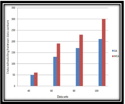
The data scheduling between data centers of three algorithms are shown in below figure.
Fig 6: Data scheduling between data centers with different number of datasets.
We can increase the number of generations then the number of data scheduling becomes smaller and smaller. The optimization results are very near to solutions.
If the number of datasets is large, the computation complexity is high in the Exhaustive search algorithm. The optimization results are infeasible, because of the computation complexity. Then we compare the results of genetic algorithm and Monte Carlo algorithm. We ran 20 different test computations randomly for 500 times on 8 data centers with different datasets. And we increase the number of data centers in different searching algorithms i.e; 20, 40, 60, and so on. The results are shown in below.
In the above graph we can compare the results of data scheduling between the data centers with the number of datasets. And now we can compare the results of data scheduling between the data centers with the number of data centers. By comparing those results such as numbers of data sets and numbers of data centers.
Fig 8: A data scheduling between data centers with different number of datasets.
From the above two figures the results are compared. The data scheduling between data centers of approximate results of genetic algorithm is smaller than results of Monte Carlo algorithm. When the number of datasets is large, the optimal solutions can be improved compared with the monte carlo algorithm.
VII. CONCLUSION
In the environment of distributed cloud computing, the data placement becomes a huge or critical issue. In genetic algorithm the optimization time is low. With the results of optimization time is low in genetic algorithm with the monte carlo algorithm.
Fig 9: Optimization time of the two algorithms in different number of data sets.
Reasonable placement of dataset in data centers can minimize the data scheduling between the data centers.
Fig 10: Optimization time of the two algorithms in different number of data centers.
In this paper a mathematical is built. The model illustrates relationship between datasets, data centers and computations. In this paper three different types of algorithms are used. The Exhaustive search algorithm is valid when the number of datasets is small. In Monte Carlo algorithm the optimization time is high. And genetic algorithm is overcome those problems in above two algorithms.
Genetic algorithm can find the optimal data placement matrix, when the numbers of data sets are large. Genetic algorithm can find an approximate optimal data placement matrix in a reasonable time, and the optimization result is better than the exhaustive search algorithm, Monte Carlo algorithm.
The focus of our research is to find the data placement matrix, and reduce the data scheduling between data centers as small as possible. In genetic algorithm the selection operator is main important. The selection operators such as Roulette wheel selection, Steady state selection, Tournament selection, and so on. In this paper we are using Roulette wheel selection, why because the selection operator in genetic algorithm affects the performance of the algorithm.
REFERENCES
[1] Introduction to cloud
computing-https://en.wikipedia.org/wiki/Cloud_computing.
[2] Data placement strategy in distributed systems
www.gsd.inesc-id.pt/~jgpaiva/pubs/ladis14-presentation.pdf
[4] Fedak, G., He, H. and Cappello, F. (2008) BitDew. A Programmable Environment for Large-Scale Data Management and Distribution. ACM/IEEE Conference on Supercomputing, Austin, 15-21 November 2008, 1-12. http://dx.doi.org/10.1109/SC.2008.5213939
[5] Kosar, T. and Livny, M. (2005) A Framework for Reliable and Efficient Data Placement in Distributed Computing Systems. Journal of Parallel and Distributed Computing,
65, 1146-1157.
http://dx.doi.org/10.1016/j.jpdc.2005.04.019
[6] Yuan, D., Yang, Y., Liu, X. and Chen, J.J. (2010) A Data Placement Strategy in Scientific Cloud Workflows. Future
Generation Computer Systems, 26, 1200-1214.
http://dx.doi.org/10.1016/j.future.2010.02.004
[7] Zheng, P., Cui, L.Z., Wang, H.Y. and Xu, M. (2010) A Data Placement Strategy for Data-Intensive Applications in Cloud. Chinese Journal of Computers, 33, 1472-1480. http://dx.doi.org/10.3724/SP.J.1016.2010.01472
[8] Labrinidis, A. and Jagadish, H. (2012) Challenges and Opportunities with Big Data. Proceedings of the VLDB Endowment,5, 2032-2033. http://dx.doi.org/10.14778/2367502.2367572
[9] Zheng, P., Cui, L.Z., Wang, H.Y. and Xu, M. (2010) A Data Placement Strategy for Data-Intensive Applications in Cloud. Chinese Journal of Computers, 33, 1472-1480.http://dx.doi.org/10.3724/SP.J.1016.2010.01472 [10] Yuan, D., Yang, Y., Liu, X. and Chen, J.J. (2010) A Data
Placement Strategy in Scientific Cloud Workflows. Future Generation Computer Systems, 26, 1200-1214. http://dx.doi.org/10.1016/j.future.2010.02.004
[11] Kosar, T. and Livny, M. (2005) A Framework for Reliable and Efficient Data Placement in Distributed Computing Systems. Journal of Parallel and Distributed Computing,
65, 1146-1157.
http://dx.doi.org/10.1016/j.jpdc.2005.04.019
[12] Agrawal, D., Das, S. and El Abbadi, A. (2011) Big Data and Cloud Computing: Current State and Future Opportunities. Proceedings of the 14th International Conference on Extending Database Technology, Uppsala, 21-25 March 2011,530-533.
[13] Exhaustive search
algorithm-www.algorithmist.com/index.php/Exhaustive_Search
[14] Monte carlo
algorithm-https://en.wikipedia.org/wiki/Monte_Carlo_algorithm [15] Grant, K. (1995) An Introduction to Genetic Algorithms.
C/C++ Users Journal, 13, 45-58.
[16] Zhou, M. and Sun, S.D. (1999) Genetic Algorithms and Applications. National Defense Industry Press, Beijing. [17] Polgar, O., Fried, M., Lohner, T. and Barsony, I. (2000)
Comparison of Algorithms Used for Evaluation of Ellipsometric Measurements Random Search, Genetic Algorithms, Simulated Annealing and Hill Climbing Graph-Searches. Surface Science, 457, 157-177. http://dx.doi.org/10.1016/S0039-6028(00)00352-6