* Corresponding author: magda.vestfalova@tul.cz
Determination of the applicability limits of the ideal gas model
for the calculation of moist air properties
Magda Vestfálová1,*, and Pavel Šafařík2
1KEZ, TU Liberec, Studentská 1402/2, 461 17 Liberec 1, Czech Republic
2CTU in Prague, FME, Department of Fluid Dynamics and Thermodynamics, Technická 4, 166 07 Praha 6, Czech Republic
Abstract.
The submitted paper deals with the finding of such moist air states in which the components of
moist air and hence the humid air itself can be described by the ideal gas model while maintaining a predefined accuracy. Both components of moist air (dry air and water vapor) can be described by a model of ideal gas at sufficiently low pressures and sufficiently high temperatures. In the paper, we are looking for such combinations of pressures and temperatures for both components, where the relative deviation in the density calculation using the ideal gas model does not exceed the desired value. In addition, on the basis of the mixture theory, such moist air conditions (characterized by pressure, temperature and specific humidity) are searched, on which the accuracy of the calculation meets the required conditions. Subsequently, diagrams are constructed that can be used to help identify the interface between a moist air area that can be described by a simple ideal gas model, and areas where it is necessary to use a more accurate model for one of the components.1 Introduction
Moist air is a mixture of dry air and water. To simplify the physical description of moist air that occurs in nature or participates in technical processes, only these components can be considered. The presence of other substances in the air (such as various gaseous pollutants, liquid components of different technologies, solids dust) will not be considered.
If all the humidity in the moist air is in gaseous state, the moist air is a homogeneous mixture. The moist air as a heterogeneous mixture contains water partly in the gas state and partly in the liquid state or partly in the gas state and partly in the solid state or partly in the gas state, partly in the liquid state and partly in the solid state.
Humidity is present in relatively small quantities in atmospheric air but is of considerable importance both in the environment and in technological processes too.
In the case of homogeneous moist air, the properties of its components are very often described by the ideal gas model. Therefore, the aim of the present paper is to determine the applicability range of this model when the ideal gas is defined [1] as a theoretical model of compressible fluid, which is characterized by the relationship between the quantities of pressure p Pa , temperature T K and density
kg m3
prT , (1)
where r
J kg 1K
is the specific gas constant, and by constant values of specific heat capacities at constantpressure
1
.const K kg J
cp
and at constant volume
1
.const K kg J
cV
.
2 Components of moist air
Dry airThe basic physical and thermodynamic properties of dry air as an ideal gas are, according to NIST (National Institute for Standards and Technology, USA) [2]:
middle molar mass:
kmol kg M 28.958 3
specific gas constant:
K kg
J r
287 .12
specific heat capacity at constant pressure:
K kg
J cp
1005 .9
specific heat capacity at constant volume:
K kg
J cV
718.8
Poisson constant:
399 . 1
0 50 100 150 200 250 300 350 400 450 500
-100 0 100 200 300 400 500 600 700 800 900 1000
temperature t [ °C ]
dens
ity
[
kg
/ m
3 ]
0.1 MPa 1 MPa 5 MPa
10 MPa 20 MPa 50 MPa
100 MPa
100 MPa
50 MPa
20 MPa 10 MPa
5 MPa 1 MPa
Fig. 1. Dependence of dry air density on pressures of MPa
1 .
0 (black), 1MPa (yellow), 5MPa (blue), 10 MPa (purple), 20 MPa (green), 50 MPa (brown) and 100 MPa (red) according to [2] (solid lines) and dependence of dry air density obtained with the ideal gas model (dashed lines).
The theoretical model of ideal gas is very advantageous for its simplicity, and is usually used to calculate the dry air properties near the atmospheric conditions. For conditions significantly different from standard atmospheric, the ideal gas model exhibits large deviations from the actual values. Figure 1 shows the actual temperature-dependence of density for selected constant pressure values (solid lines) and for a comparison of the same dependences obtained with the ideal gas model (dashed lines).
It can be seen that the ideal gas model is useful for calculating the density of dry air at low pressures and high temperatures. With increasing pressure and decreasing temperature, the differences between actual density and density calculated using the ideal gas model increase.
Figure 2 shows relative dry air density deviations calculated using the ideal gas model for the same pressures as were used in Figure 1. The area of possible use of the ideal gas model depends on the required accuracy: if we would consider the accuracy of 10 % to be sufficient, it is possible to use the ideal gas model to calculate the dry air density up to pressures of 20 MPa
(for temperatures higher than 50 C ) (for pressures of MPa
50 and 100 MPa , the ideal gas model in the entire
temperature range of 150 C to 1000 C gives
deviations greater than 10 % ). However, if we require an accuracy of up to 1% , it would be possible to use the ideal gas model to calculate the dry air density only
within a certain range of pressures and temperatures. For example, for a pressure of 0.1MPa , the ideal gas model
is usable for temperatures above about 140 C , for
a pressure of 1MPa is usable for temperatures above
about 25 C , for a pressure of 5MPa in a temperature
range of 25C to 105 C , for a pressure of 10 MPa
only in a temperature range of 25 C to 75C .
-5 -4 -3 -2 -1 0 1 2 3 4 5 6 7 8 9 10
-200 0 200 400 600 800 1000
temperature t [ °C ]
re
lat
ive d
ev
iat
io
n
of
DA
[
% ]
0.1 MPa 1 MPa 5 MPa
10 MPa 20 MPa 20 MPa
10 MPa
5 MPa
1 MPa
0.1 MPa
Fig. 2. The course of relative deviations of dry air densities as an ideal gas in dependence on temperature for pressures of
MPa
1 .
0 (black), 1MPa (yellow), 5MPa (blue), 10 MPa (purple), 20 MPa (green), 50 MPa (brown) a 100 MPa (red).
Water is a relatively complex substance from a thermodynamic point of view. It is the most widely used and best available energy transfer medium. Therefore, extensive research has focused on it. For the work of experts, documents are gradually approved by the International Association for Properties of Water Steam (IAPWS) as recommendations for determination of thermodynamic and thermophysical properties of water and water vapour. Important documents are:
1995 (revision 2014) – Formulation of the thermodynamic properties of a common water substance for general and scientific use (in short IAPWS-95),
1997 – New international formulation of thermodynamic properties of water and steam for industrial purposes (in short IAPWS IF-97). The state equations of water and water vapour according to these two documents are substantially distant from the state equation of the ideal gas.
0 50 100 150 200 250 300 350 400 450 500
-100 0 100 200 300 400 500 600 700 800 900 1000
temperature t [ °C ]
dens ity [ kg / m
3 ]
0.1 MPa 1 MPa 5 MPa
10 MPa 20 MPa 50 MPa
100 MPa 100 MPa 50 MPa 20 MPa 10 MPa 5 MPa 1 MPa
Fig. 1. Dependence of dry air density on pressures of MPa
1 .
0 (black), 1MPa (yellow), 5MPa (blue), 10 MPa (purple), 20 MPa (green), 50 MPa (brown) and 100 MPa (red) according to [2] (solid lines) and dependence of dry air density obtained with the ideal gas model (dashed lines).
The theoretical model of ideal gas is very advantageous for its simplicity, and is usually used to calculate the dry air properties near the atmospheric conditions. For conditions significantly different from standard atmospheric, the ideal gas model exhibits large deviations from the actual values. Figure 1 shows the actual temperature-dependence of density for selected constant pressure values (solid lines) and for a comparison of the same dependences obtained with the ideal gas model (dashed lines).
It can be seen that the ideal gas model is useful for calculating the density of dry air at low pressures and high temperatures. With increasing pressure and decreasing temperature, the differences between actual density and density calculated using the ideal gas model increase.
Figure 2 shows relative dry air density deviations calculated using the ideal gas model for the same pressures as were used in Figure 1. The area of possible use of the ideal gas model depends on the required accuracy: if we would consider the accuracy of 10 % to be sufficient, it is possible to use the ideal gas model to calculate the dry air density up to pressures of 20 MPa
(for temperatures higher than 50 C ) (for pressures of MPa
50 and 100 MPa , the ideal gas model in the entire
temperature range of 150 C to 1000 C gives
deviations greater than 10 % ). However, if we require an accuracy of up to 1% , it would be possible to use the ideal gas model to calculate the dry air density only
within a certain range of pressures and temperatures. For example, for a pressure of 0.1MPa , the ideal gas model
is usable for temperatures above about 140 C , for
a pressure of 1MPa is usable for temperatures above
about 25C , for a pressure of 5MPa in a temperature
range of 25C to 105 C , for a pressure of 10 MPa
only in a temperature range of 25 C to 75 C .
-5 -4 -3 -2 -1 0 1 2 3 4 5 6 7 8 9 10
-200 0 200 400 600 800 1000
temperature t [ °C ]
re lat ive d ev iat io n
of
DA
[
% ]
0.1 MPa 1 MPa 5 MPa
10 MPa 20 MPa 20 MPa
10 MPa
5 MPa
1 MPa
0.1 MPa
Fig. 2. The course of relative deviations of dry air densities as an ideal gas in dependence on temperature for pressures of
MPa
1 .
0 (black), 1MPa (yellow), 5MPa (blue), 10 MPa (purple), 20 MPa (green), 50 MPa (brown) a 100 MPa (red).
Water is a relatively complex substance from a thermodynamic point of view. It is the most widely used and best available energy transfer medium. Therefore, extensive research has focused on it. For the work of experts, documents are gradually approved by the International Association for Properties of Water Steam (IAPWS) as recommendations for determination of thermodynamic and thermophysical properties of water and water vapour. Important documents are:
1995 (revision 2014) – Formulation of the thermodynamic properties of a common water substance for general and scientific use (in short IAPWS-95),
1997 – New international formulation of thermodynamic properties of water and steam for industrial purposes (in short IAPWS IF-97). The state equations of water and water vapour according to these two documents are substantially distant from the state equation of the ideal gas.
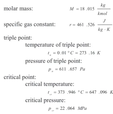
The basic physical properties of water and water vapour are according to [3]:
molar mass:
kmol kg M 18.015
specific gas constant:
K kg
J r
461 .526
triple point:
temperature of triple point:
K C
ttr0.01 273 .16 pressure of triple point:
Pa ptr611 .657
critical point:
critical temperature:
K C
tcr373.946 647.096
critical pressure:
MPa pcr22.064
The thermodynamic behaviour of water occurring in homogeneous moist air (i.e. water vapour) can be described under normal atmospheric conditions by the ideal gas model.
The basic thermodynamic properties of water vapour as an ideal gas:
specific heat capacity at constant pressure:
K kg
J cp
1898 .56
specific heat capacity at constant volume:
K kg
J cV
1398 .56
Poisson constant: 33 . 1
For thermodynamics of humid air, it is important to determine the thermodynamic properties of water vapour within the limits of saturation.
On the liquid-steam saturation limit from the triple point to the critical point, the scientific formulation (IAPWS 95) [4] determines the dependence of the saturated water vapour pressure on the temperature function
5 , 7 6 4 5 5 , 3 4 3 3 5 , 1 2 1 1 1 exp a a a a a a p p cr, (2)
where: cr T T 1 (3)
is the temperature function,
K
T is the temperature,
the constants in equation (2) are given in Table 1.
Table 1. Constants in equation (2).
1
a 7.859 517 83 a4 22.680 7411
2
a 1.844 082 59 a5 15.961 871 9
3
a 11.786 649 7 a6 1.801 225 02
On the saturation limit between the solid and gaseous phases H2O, i.e. for sublimation and desublimation, the
pressure in relation to the temperature from 50 K to the
triple point is solved according to equation [5]
3 1 1 exp i i b i tr a p
p , (4)
where:
tr T
T
, (5)
is the temperature function, T K is the temperature,
the constants in equation (4) are given in Table 2.
Table 2. Constants in equation (4).
1
a 21.214 400 6 b1 0.003 333 333 33
2
a 27.320 3819 b2 1.206 666 67
3
a 6.105 9813 b3 1.703 333 33
Similarly to dry air, it is advantageous to describe the properties of water steam be the ideal gas model. The scope of application of the ideal gas model is limited by the beginning of condensation, it is by achieving a saturation state (a condition where moist air becomes a heterogeneous mixture, it is when water begins excreted from moist air in the form of a liquid or solid phase), and next by the range of pressures and temperatures where the steam is a homogeneous mixture, but the ideal gas model has large deviations from actual data. Figure 3 shows the actual dependence of density of water vapor at the temperature for selected constant pressure values (full line) and, for comparison, the same dependence obtained using the ideal gas model (dashed lines).
Similarly to dry air, at lower pressures, the ideal gas model produces results comparable to real values, even up to the saturation curve. At higher pressures, the densities calculated using the ideal gas model deviate from the actual properties near the saturation curve, and for very high pressures, the ideal gas model does not produce the right results even at high temperatures.
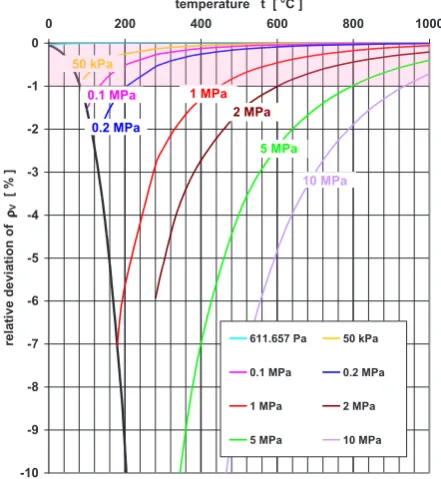
Figure 4 shows relative water vapor density deviations calculated using the ideal gas model for the pressures used in Figure 3. As with dry air, the area of possible use of the ideal gas model depends on the required accuracy: if we would consider the accuracy of
%
10 to be sufficient, it is possible to use the ideal gas model to calculate the water vapor density up to pressure of 2MPa and it up to the saturation curve, or even up to
pressure of 10 MPa for temperatures over 500 C .
However, if we require an accuracy of up to 1% , it would be possible to use the ideal gas model to calculate the water vapor density only up to pressure about
kPa
50 (an accuracy of up to 1% would be met up to the saturation vaporous state), or to pressure about
MPa
1 .
0 , but only for temperatures higher than about
C
135 , or to pressure about 0.2MPa , but only for
temperatures higher than about 205 C ; at a pressure of MPa
0 1 2 3 4 5 6
0 200 400 600 800 1000
temperatura t [ °C ]
dens
ity
[
kg
/ m
3 ]
611.657 Pa
50 kPa
0.1 MPa
0.2 MPa
0.5 MPa
1 MPa
2 MPa 2 MPa
1 MPa
0.5 MPa
0.2 MPa
0.1 MPa
50 kPa
Fig. 3. The dependence of the density of water vapor at the temperature for pressures 611.657 Pa (light blue), 50 kPa (yellow), 0.1MPa (purple), 0.2MPa (blue), 0.5MPa (green), 1MPa (red) and 2MPa (brown) according to [3] (solid lines) and the dependence of water vapor density obtained with the ideal gas model (dashed lines).
3 Moist air
Moist air as a thermodynamic system is a mixture of dry air and water substances. The water contained in the moist air is always in the form of steam, but in addition (in the case of a heterogeneous mixture), part of the water in moist air may also be in a liquid or solid state.
Temperature of moist air tMA C is equal to the
temperature of its components
t t t
tMA DA V . (6)
Pressure of moist air pMA Pa is equal according to
Dalton's law to the sum of the partial pressures of dry air and water vapor
pMApDA pV . (7)
Mass of moist air mMA kg is equal
O H DA
MA m m
m 2 . (8)
Density of moist air
3
m kg MA is the ratio of the mass of moist air to its volume, it is provided that the water in the humid air is only as vapor
V DA
MA
. (9)
Pressure of saturated water vapor pV Pa is
a significant variable for moist air, which determines the water content limit in the air for the existence of a homogeneous mixture:
- if pV pV, the moist air is unsaturated and the
mixture homogeneous;
- if pV pV, the moist air is saturated and the
mixture homogeneous;
- if pV pV, the moist air is supersaturated and
the mixture is heterogeneous.
Pressure of saturated water vapor is a function of temperature
t p
pV V , (10)
(see equation (2), (4)).
Dew point temperature tDP C is the moist air
temperature at which the moist air reaches the saturation state under isobaric cooling
V DP
V t p t
p , (11)
it is the water vapor contained therein is in the state of saturated vapor.
-10 -9 -8 -7 -6 -5 -4 -3 -2 -1
00 200 400 600 800 1000
temperature t [ °C ]
re
lat
ive d
ev
iat
io
n
of
V
[
% ]
611.657 Pa 50 kPa
0.1 MPa 0.2 MPa
1 MPa 2 MPa
5 MPa 10 MPa
10 MPa
5 MPa 2 MPa
1 MPa
0.2 MPa
0.1 MPa
50 kPa
Fig. 4. The course of relative deviations of water vapor densities as an ideal gas in dependence on temperature for pressures of 611 .657 Pa (light blue), 50 kPa (yellow),
MPa
1 .
0 (purple), 0.2MPa (blue), 1MPa (red), 2MPa (brown), 5MPa (green) a 10 MPa (violet).
Absolute air humidity
3
m kga is the mass amount
of steam in unit air volume. It's the vapor density V at
vapor pressure pV and temperature t. Absolute
humidity is defined only for a homogeneous mixture and for given temperature can be within a range
t
a V.
;
0 .
Relative air humidity is the ratio of absolute humidity to absolute humidity of saturated humid air at a given temperature
a a
0 1 2 3 4 5 6
0 200 400 600 800 1000
temperatura t [ °C ]
dens ity [ kg / m
3 ]
611.657 Pa 50 kPa 0.1 MPa 0.2 MPa 0.5 MPa 1 MPa 2 MPa 2 MPa 1 MPa 0.5 MPa 0.2 MPa 0.1 MPa 50 kPa
Fig. 3. The dependence of the density of water vapor at the temperature for pressures 611.657 Pa (light blue), 50 kPa (yellow), 0.1MPa (purple), 0.2MPa (blue), 0.5MPa (green), 1MPa (red) and 2MPa (brown) according to [3] (solid lines) and the dependence of water vapor density obtained with the ideal gas model (dashed lines).
3 Moist air
Moist air as a thermodynamic system is a mixture of dry air and water substances. The water contained in the moist air is always in the form of steam, but in addition (in the case of a heterogeneous mixture), part of the water in moist air may also be in a liquid or solid state.
Temperature of moist air tMA C is equal to the
temperature of its components
t t t
tMA DA V . (6)
Pressure of moist air pMA Pa is equal according to
Dalton's law to the sum of the partial pressures of dry air and water vapor
pMApDA pV . (7)
Mass of moist air mMA kg is equal
O H DA
MA m m
m 2 . (8)
Density of moist air
3
m kg MA
is the ratio of the
mass of moist air to its volume, it is provided that the water in the humid air is only as vapor
V DA
MA
. (9)
Pressure of saturated water vapor pV Pa is
a significant variable for moist air, which determines the water content limit in the air for the existence of a homogeneous mixture:
- if pV pV, the moist air is unsaturated and the
mixture homogeneous;
- if pV pV, the moist air is saturated and the
mixture homogeneous;
- if pV pV, the moist air is supersaturated and
the mixture is heterogeneous.
Pressure of saturated water vapor is a function of temperature
t p
pV V , (10)
(see equation (2), (4)).
Dew point temperature tDP C is the moist air
temperature at which the moist air reaches the saturation state under isobaric cooling
V DP
V t p t
p , (11)
it is the water vapor contained therein is in the state of saturated vapor. -10 -9 -8 -7 -6 -5 -4 -3 -2 -1
00 200 400 600 800 1000
temperature t [ °C ]
re lat ive d ev iat io n of V [ % ]
611.657 Pa 50 kPa
0.1 MPa 0.2 MPa
1 MPa 2 MPa
5 MPa 10 MPa
10 MPa 5 MPa 2 MPa 1 MPa 0.2 MPa 0.1 MPa 50 kPa
Fig. 4. The course of relative deviations of water vapor densities as an ideal gas in dependence on temperature for pressures of 611 .657 Pa (light blue), 50 kPa (yellow),
MPa
1 .
0 (purple), 0.2MPa (blue), 1MPa (red), 2MPa (brown), 5MPa (green) a 10 MPa (violet).
Absolute air humidity
3
m kg
a is the mass amount
of steam in unit air volume. It's the vapor density V at
vapor pressure pV and temperature t. Absolute
humidity is defined only for a homogeneous mixture and for given temperature can be within a range
t
a V.
;
0 .
Relative air humidity is the ratio of absolute
humidity to absolute humidity of saturated humid air at a given temperature
a a
. (12)
Relative humidity is defined only for a homogeneous mixture and may be within the range 0;1 . Assuming water vapor contained in moist air can be described by the ideal gas model
V V p p
. (13)
Specific air humidity
1
DA
V kg kg
x is the ratio of the
mass of water to the dry air mass DA O H m m
x 2 . (14)
In the case of a homogeneous mixture in which water is contained in the air only in the vapor form
DA V DA V m m x
. (15)
Specific gas constant of moist air
1 1
kg K
J
rMA is
equal
MA DA rV x x r x r 1 1 1 (16)
and specific heat capacity at constant pressure of moist air
1 1
kg K
J c
MA
p is equal
pMA pDA cpV x x c x c 1 1 1
. (17)
So that thermodynamic constant of moist air as and ideal gas depend on specific humidity x; at xconst . they are constant.
If the moist air forms a homogeneous mixture and its components (dry air and steam) can be described by the ideal gas model, it is possible to derive the relationship between specific and relative humidity
V MA V p p p x
0.622 , (18)
resp. V MA V p p p x 622 .
0 . (19)
For the specific humidity of the saturated homogeneous mixture 1
t x t p p t p x V MA
V
0.622 . (20)
Our task is to find a boundaries in moist air (combination of pressure, temperature and humidity), where there is possible to use the ideal gas model to calculate the properties of components of the moist air with sufficient accuracy.
One limit is the boundary on which ends the existence of water in the form of steam only. The paper [6] deals by searching for this boundary: For a given value of specific humidity of moist air, the dependence of saturated pressure of moist air on the temperature was solved from equations (20) and (2), respectively at the case of sublimation limit may be (4). In the equilibrium
T
p diagram, a curve (with a parameter of the specific
humidity x) was constructed, on which water would be
excreted from moist air (the curves of the saturated moist air for different water contents, it is for different values of specific humidity x), see Figure 5.
1.E+04 1.E+05 1.E+06 1.E+07 1.E+08
0 50 100 150 200
temperature t [ °C ]
pr
essu
re p
[ P a ] x=0.001 x=0.01 x=0.1
Fig. 5. Curves of saturated moist air for different values of specific humidity x [6].
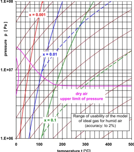
The aim of this paper is to find additional limits (it means the areas of states of the homogeneous moist air), where both components can be described by the ideal gas model with the required accuracy.
The curves in Figure 5 show the states of saturated (it means homogeneous) moist air for three different values of specific humidity x. The vapor contained in the
saturated moist air is in the form of saturated vapor. However, according to Figure 4, the ideal gas model used for vapor exhibits increasing deviations, when the pressure increases. So, for higher pressures, on the curves in the diagram in Figure 5 there are although the homogeneous states of moist air, but if we want to keep the necessary accuracy, it is no longer possible to describe the water vapor contained in the moist air by the ideal gas model!
For the desired maximum deviation, it is possible to find in the diagram in Figure 4 the dependence of partial pressure of vapor on temperature. Then, for the selected specific humidity x, we calculate from the relation (18)
the maximum pressure of the humid air, at which the density of the water vapor contained in the moist air at a given temperature and at given specific humidity can be calculated using the ideal gas model (when the required accuracy is achieved). The obtained curve ends in the pT diagram on the saturated moist air curve
corresponding to the given specific humidity x. In
Figures 6, 7 and 8, these curves are plotted with a dashed line of the same color as the saturated moist air curves for the corresponding value of specific humidity x.
Thus, if the state of moist air of a given specific humidity in the pT diagram is to the right of the
required accuracy; between the two curves is the area where the moist air is still homogeneous, but for calculating the vapor properties it is necessary to use one of the more precise models; to the left of the saturated moist air curves, the humid air is already heterogeneous.
1.E+05 1.E+06 1.E+07 1.E+08
0 100 200 300 400 500
temperature t [ °C ]
pr
essu
re p
[
P
a ]
x = 0.001
x = 0.01
x = 0.1
dry air upper limit of pressure
Range of usability of the model of ideal gas for humid air
(accuracy: to 1%)
Fig. 6. Area of usability of the ideal gas model for the calculation of properties of components of moist air at the required accuracy of the calculation to 1% for specific
humidity x of 0.1, 0.01 and 0.001 .
Other limit, which have to be found, is the field of application of the ideal gas model for dry air contained in the moist air. As in the case of water vapor, we can find in the diagram in Figure 2 the dependence of dry air partial pressure on the temperature for the desired maximum relative deviation. By adjusting the equation (18) the relationship between the pressure of moist air, specific humidity and partial pressure of dry air can be obtained
622 . 0 1 x
p
pMA DA , (21)
from which we can calculate the maximum moist air pressure for the selected specific humidity x in which the density of the dry air contained in the moist air at a given temperature and specific humidity can be calculated using the ideal gas model to meet the required accuracy.
In Figure 6, for the selected values of specific humidity x is plotted line (dotted curve) of maximum pressure of moist air at which it is possible to calculate the partial dry air density using the ideal gas model, while meeting the required accuracy. It can be seen from the Figure 6 that the upper limit of pressure of moist air
depends very little on the specific humidity x and the curves almost coincide with the dry air partial pressure curve (for the maximum humidity used by us: x0.1,
the total pressure is equal to 1.16 times the dry air partial pressure; for humidity x0.01 is equal to 1.016 times
and for humidity x0.001 it's just 1.0016 times). Thus,
in the diagram in Figure 6, the dependence of the maximum dry air partial pressure on the temperature to fulfill the required accuracy is plotted. This curve is only a little different from the curves describing the total pressure of moist air for the selected values of specific humidity x. In the other figures, therefore, only the dependence of dry air partial pressure is plotted for expression of boundary of usability of model of ideal gas for dry air.
1.E+06 1.E+07 1.E+08
0 100 200 300 400 500
temperature t [°C]
pr
essu
re p
[
P
a ]
x = 0.001
x = 0.01
x = 0.1
dry air upper limit of pressure
Range of usability of the model of ideal gas for humid air
(accuracy: to 2%)
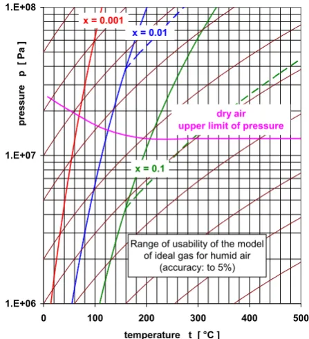
Fig. 7. Area of usability of the ideal gas model for the calculation of properties of components of moist air at the required accuracy of the calculation to 2% for specific
humidity x of 0.1, 0.01 and 0.001 .
Thus, if the state of moist air is in the pT diagram shown by a point below the maximum dry air partial pressure curve, the partial density of the dry air (contained in the moist air) may be calculated with sufficient precision using the ideal gas model.
required accuracy; between the two curves is the area where the moist air is still homogeneous, but for calculating the vapor properties it is necessary to use one of the more precise models; to the left of the saturated moist air curves, the humid air is already heterogeneous.
1.E+05 1.E+06 1.E+07 1.E+08
0 100 200 300 400 500
temperature t [ °C ]
pr
essu
re p
[
P
a ]
x = 0.001
x = 0.01
x = 0.1
dry air upper limit of pressure
Range of usability of the model of ideal gas for humid air
(accuracy: to 1%)
Fig. 6. Area of usability of the ideal gas model for the calculation of properties of components of moist air at the required accuracy of the calculation to 1% for specific
humidity x of 0.1, 0.01 and 0.001 .
Other limit, which have to be found, is the field of application of the ideal gas model for dry air contained in the moist air. As in the case of water vapor, we can find in the diagram in Figure 2 the dependence of dry air partial pressure on the temperature for the desired maximum relative deviation. By adjusting the equation (18) the relationship between the pressure of moist air, specific humidity and partial pressure of dry air can be obtained
622 . 0 1 x
p
pMA DA , (21)
from which we can calculate the maximum moist air pressure for the selected specific humidity x in which the density of the dry air contained in the moist air at a given temperature and specific humidity can be calculated using the ideal gas model to meet the required accuracy.
In Figure 6, for the selected values of specific humidity x is plotted line (dotted curve) of maximum pressure of moist air at which it is possible to calculate the partial dry air density using the ideal gas model, while meeting the required accuracy. It can be seen from the Figure 6 that the upper limit of pressure of moist air
depends very little on the specific humidity x and the curves almost coincide with the dry air partial pressure curve (for the maximum humidity used by us: x0.1,
the total pressure is equal to 1.16 times the dry air partial pressure; for humidity x0.01 is equal to 1.016 times
and for humidity x0.001 it's just 1.0016 times). Thus,
in the diagram in Figure 6, the dependence of the maximum dry air partial pressure on the temperature to fulfill the required accuracy is plotted. This curve is only a little different from the curves describing the total pressure of moist air for the selected values of specific humidity x. In the other figures, therefore, only the dependence of dry air partial pressure is plotted for expression of boundary of usability of model of ideal gas for dry air.
1.E+06 1.E+07 1.E+08
0 100 200 300 400 500
temperature t [°C]
pr
essu
re p
[
P
a ]
x = 0.001
x = 0.01
x = 0.1
dry air upper limit of pressure
Range of usability of the model of ideal gas for humid air
(accuracy: to 2%)
Fig. 7. Area of usability of the ideal gas model for the calculation of properties of components of moist air at the required accuracy of the calculation to 2% for specific
humidity x of 0.1, 0.01 and 0.001 .
Thus, if the state of moist air is in the pT diagram shown by a point below the maximum dry air partial pressure curve, the partial density of the dry air (contained in the moist air) may be calculated with sufficient precision using the ideal gas model.
The area where the densities of the both components of moist air can be calculated using the equation state of the ideal gas lies in the pT diagrams "bottom right": it is bounded by a saturated moist air curve for the corresponding specific humidity x, by a curve showing the maximum value of the air pressure (at given temperature and specific humidity x), when it is possible to model water vapor with the ideal gas model, and by a curve showing the maximum pressure value (at
given temperature) when it is possible to model dry air with the ideal gas model.
1.E+06 1.E+07 1.E+08
0 100 200 300 400 500
temperature t [ °C ]
pre
ss
ure
p
[ P
a ]
x = 0.001
x = 0.01
x = 0.1
dry air upper limit of pressure
Range of usability of the model of ideal gas for humid air
(accuracy: to 5%)
Fig. 8. Area of usability of the ideal gas model for the calculation of properties of components of moist air at the required accuracy of the calculation to 5% for specific
humidity of 0.1, 0.01 and 0.001 .
Figure 6 shows an area in which the ideal gas model achieves an accuracy of 1% , in Figure 7 an area with
accuracy of 2% , and in Figure 8 an area with accuracy
of 5% .
In all of the figures, an isentropy network (a set of brown curves) is plotted for better idea:
1) If the reversible adiabatic compression occurs in homogeneous moist air, the moist air will "move away" from the saturation curve, it means: it is not possible to get from homogeneous moist air to heterogeneous moist air during isentropic compression, on the other hand, in a reversible adiabatic expansion, it is possible to reach a state of saturated moist air.
2) If the reversible adiabatic compression occurs in homogeneous moist air, the accuracy of the description of the water vapor properties by the ideal gas model will be increased ("we move away" from boundaries limiting the usability of the ideal gas model for steam water), but the accuracy of the calculation of the dry air properties by the ideal gas model will be reduced; in reversible adiabatic compression it is possible to cross the boundary where the ideal gas model is still usable for calculating the dry air properties.
3) In reversible adiabatic expansion, the accuracy of the ideal gas model for the dry air contained in moist air increases; the accuracy of the ideal gas model for the water vapor contained in moist air reduces, but not too significantly - the curve limiting the pressure of moist air for using the ideal gas model for the water vapor has
only a slightly greater slope than the isentropic curves; The main "danger" in reversible adiabatic expansion in moist air is the possibility of reaching the condensation boundary.
Conclusion
In the equilibrium pT diagram, the boundary of range of usability of the ideal gas model for the calculation of properties of components of moist air were constructed for different relative accuracy values (1% , 2% , 5% ).
Once the boundary is reached, a more accurate model is required to use (for calculation of properties of the components of moist air) for preserve the accuracy of calculation.
Acknowledgment
This publication was written at the Technical University of Liberec, Faculty of Mechanical Engineering with the support of the Institutional Endowment for the Long Term Conceptual Development of Research Institutes, as provided by the Ministry of Education, Youth and Sports of the Czech Republic in the year 2017.
The second author, P.Šafařík, expresses thanks for
support from the Project No. CZ.2.16/3.100/21569 Centre 3D Volumetric Anemometry.
References
1. P. Šafařík, M. Vestfálová, Thermodynamics of Moist Air, CTU Publishing House (in Czech) (2016) 2. E.W. Lemmon, R.T. Jacobsen, S.G. Penoncello,
D.G. Friend, Journal of Physical and Chemical Reference Data, 29, 3: 331-385 (2000)
3. O. Šifner, J. Klomfar, International Standards of Thermophysical Properties of Water and Steam, Academia (in Czech) (1996)
4. IAPWS: Revised Release on the IAPWS
Formulation 1995 for the Thermodynamic Properties of Ordinary Water Substance for General and Scientific Use (2014)
5. IAPWS: Revised Release on the Pressure along the Melting and Sublimation Curves of Ordinary Water Substance (2011)
![Fig. 1. Dependence of dry air density on pressures of 0.1MPa (black), 1MPa (yellow), 5MPa (blue), 10MPa (purple), 20MPa (green), 50MPa (brown) and 100MPa (red) according to [2] (solid lines) and dependence of dry air density obtained with the ideal gas mod](https://thumb-us.123doks.com/thumbv2/123dok_us/8046990.1340368/2.595.61.282.75.342/dependence-density-pressures-yellow-according-dependence-density-obtained.webp)
![Fig. 5. Curves of saturated moist air for different values of specific humidity x [6]](https://thumb-us.123doks.com/thumbv2/123dok_us/8046990.1340368/5.595.310.535.87.293/fig-curves-saturated-moist-different-values-specific-humidity.webp)