Bayesian Analysis of Competing Risks Models with Masked Causes of Failure and Incomplete Failure Times
Yosra Yousif 1, Faiz A. M. Elfaki 2,* and Meftah Hrairi 1
1 Department of Mechanical Engineering, Faculty of Engineering, International Islamic
University Malaysia (IIUM), P.O. Box 10, 50728 Kuala Lumpur, Malaysia
2 Department of Mathematics, Statistics and Physics, College of Arts and Sciences, Qatar
University, P.O. Box 2713, Doha, Qatar
* E-mail: [email protected]
Abstract
Bayesian analysis for masked data under competing risk frameworks is studied for the purpose of assessing the impact of covariates on the hazard functions when the failure time is exactly observed for some subjects but only known to lie in an interval of time for the remaining subjects. Such data, known as partly interval-censored data, usually result from periodic inspection. Dirichlet and Gamma processes are assumed as priors for masking probabilities and baseline hazards. The Markov Chain Monte Carlo (MCMC) technique is employed for the implementation of the Bayesian approach. The effectiveness of the proposed model is tested through numerical studies, including simulated and real data sets.
Keywords: competing risks; masked causes of failure; Markov Chain Monte Carlo; Bayesian analysis; partly interval censored
1. Introduction
Suppose we have a unit subjected to causes of failure under study. Let T be the time until the unit experiences failure due to one of the causes. It often happens that there are a few unidentified causes responsible for the unit’s failure. Such type of incomplete data is generally referred to as masked data. Why a unit fails can only be identified up to a Minimum Random Subset (MRS) S ⊆ {1, … , K}. If the precise cause of failure is identified as , then S = {K} is a singleton. If the cause of failure is not identified, then S = {1, … , K} resulting in full masking of the cause. Thus, every detected failure time ,i = 1, … , N, is accompanied by a detected MRS denoted by . However, another reason for incomplete detections could be because the exact failure time T is not known.
Work on masked data is in abundance in the literature, Miyakawa (1984) provided maximum likelihood estimates (MLEs) with two causes of failure and independent exponential failure-times when the data is masked and uncensored. Dinse (1986) suggested nonparametric maximum likelihood estimators of prevalence and mortality when the MRS is a known cause or a full masked cause. Reiser et al. (1995) presented a Bayesian analysis assuming exponentially distributed component lifetimes, and Guttman et al. (1994) took this work further to the case where the masking probability depends on the actual cause of failure. Considering the partial masking cases, Mukhopadhyay & Basu (1997) studied a Bayesian analysis with independent Weibull distributions and made the assumption of similar shape structures for all the K risks. Basu et al. (1999) on the other hand, developed a Bayesian analysis for masked data from a general K component system with non-identical Weibull distributions. Further, they investigated a Bayesian analysis based on a general flexible parametric framework for complex forms of censoring (Basu et al. 2003). Without the symmetry assumption, Kuo & Yang (2000) developed a Bayesian analysis with
independent exponential as well as Weibull distributions, while Mukhopadhyay & Basu (2007) studied the case of a series system, the components of which possess independent log-normal life distribution. Xu & Tang (2011) considered a nonparametric Bayesian approach for masked data which extended the findings of Neath & Samaniego (1996) to series systems comprising some masked competing risks. In contrast, based on a cause-specific formulation, Flehinger et al. (2002) proposed an approach of completely parametric cause-specific hazards using stage 1 and stage 2 information when the failure times for the competing risks have a Weibull distribution. Craiu & Reiser (2006) developed an EM-based method that allowed dependent competing risks and produced estimators for the sub-distribution functions. Moreover, Lu & Tsiatis (2001) presented parametric models to estimate the regression coefficients where by the cause-specific hazard for the cause of interest is associated with the covariates through a proportional hazards relationship. Sen et al. (2010) introduced a semi-parametric Bayesian approach discussing three different models using variety in priors. Yosra, et al. (2016) discussed partly interval-censored data under competing risks framework when the cause of failure might be masked, and compared their result with Sen’s models.
In engineering field, researchers often show interest in component reliability. Therefore, most of the work mentioned above was developed for masked data based on the series system formulation considering the cases where the failure time is complete (no censored units), right-censored (RC) or interval-censored. Nevertheless, one can be interested in studying the impact of the risk factors on the hazard function other than the estimation of reliability.
Since the covariates’ effect is of interest, a Bayesian analysis under cause-specific hazard framework is considered in this paper employing Cox proportional hazards model, which is used extensively but mostly for public health studies (see (Han et al. 2017) and (Liu et al. 2017)) . We investigate the case where the data are masked and the failure time is partly interval-censored (PIC). This work can be regarded as a development of Sen et al.'s (2010) model. Section 2 and 3 introduce the model construction and the Bayesian computation techniques. Section 4 provides some results using simulated data to evaluate the model performance, while section 5 illustrates our approach using an actual data set, while section 6 concludes this paper.
2. Model Structure
In the case of masked data, for each unit, we not only observe the failure time but also a set of causes that include the true cause of failure. Assume that we observe N units each has K causes of failure acting on it. Let X denote the observed collection of covariates. Then for any unit , we observe the vector ( , , ), where denotes the failure time and denotes the MRS of causes that are possibly responsible for the unit failure. For the unit, the likelihood contribution from the data ( , , ) consists of P( , | ), Kuo & Yang (2000) and can be expressed as
P( , | ) = P( , = | )P( | , = , ), j = 1, … , K ,
where denotes the actual cause of failure of the unit. Note that P( , = | ) = ( | ). Then when the observation of C is incomplete, see Martin J. Crowder (2001), the likelihood contribution for an observed failure can be modified to;
P( , | )
∈
= ( | )P( | , = , ).
∈
time of the unit ( ∈( , ]). If the unit failure occurred before the first inspection time, then
we have a left-censored observation ( ∈(0, ]) and if the unit did not fail until the last inspection time, then we have a right-censored observation ( ∈( ,∞]). Define δ , γ as censoring indicators taking the value of one if the failure time T is left-censored or interval-censored and taking a value of zero otherwise. Then, the likelihood contribution of the unit when the observation of T is incomplete can be expressed as;
= ( | ) [ ( | ) − ( | )]
= ( | ) [1 − ( | )] [( ( | ) ( | )⁄ ) − 1] [ ( | )] ,
where , ( + = ) are the numbers of the units whose failure time is exact and interval-censored (including left- and right-interval-censored), respectively.
In this study, our interest is in the semi-parametric Bayesian estimation of the regression coefficients. Therefore, we prefer to work with the cause-specific formulation utilizing the popular proportional hazards (PH) model that is;
λ(T, X) =λ (T)eβ′ , j = 1, … , K , (2.1)
where λ , β are, respectively, the baseline hazard and the regression coefficient of the cause of failure, and X represents the vector of the explanatory variables.
In this study, where both failure time and cause of failure are incomplete, we need to consider the two cases discussed above to formulate the likelihood function. Let , , ( + + =
) denote the numbers of the units whose failure times are exact, right-censored, and interval-censored (including left-interval-censored) respectively. Then the full likelihood of masked and partly interval-censored data can be expressed as;
L = P(S|T , C = j, X)f (T|X)
∈
S(L |X )
× P(S|T , C = j, X )[F (R |X ) − F (L|X)]
∈
L = P(S|T , C = j, X )λ (T|X ) ∑ X
∈
× ∑ X
× P(S|T , C = j, X)[ λ (t|X )e ∑ sX dt
∈
− λ (t|X)e ∑ sX dt] (2.2)
= P(S|T , C = j, X)λ (T ) ′ ∑ ( )
′
∈
× ∑ X
× P(S|T , C = j, X )[ λ (t) ′ e ∑ ( )
′
dt
∈
− λ (t) ′ e ∑ ( )
′
dt] (2.3)
When dealing with the masked data, many researchers adopt the symmetry assumption that involves an equal chance of detecting a similarly masked subset of causes regardless of the actual cause, that is;
P(S|T , C = j, X ) = P(S T , C = j′, X ), j, j′ ∈ S (2.4)
The assumption (2.4) makes the analysis proceed with less likelihood that is not reliant on masking probabilities. In this paper, we introduce a Bayesian analysis using the full likelihood (2.3). We model the masking probabilities to be autonomous of the failure time but dependent on cause of failure. Moreover, we allow them to depend on subject-level covariates.
It is often of interest to determine the cause that is responsible for the unit failure when it is masked. To determine this cause, we need to compute the diagnostic probability, which is the probability of the i risk, causing the unit to fail given the observed masking set and the unit’s failure time. According to our full likelihood, we have two different ways to compute the diagnostic probabilities depending on whether the failure time of the unit is exact or interval-censored (including left-censored). First, when the i unit is exact, the diagnostic probability can be defined as;
P(C = j|S , T , X ) = P(S|T , C = j, X )f (T|X)
∑∈ P(S|T , C = l, X)f (T|X ), j ∈ S (2.5) Second, when the i unit is interval-censored, the diagnostic probability can be defined as;
P(C = j|S , T , X) = ∑ P(S|T , C = j, X) F (R |X) − F (L|X ) P(S|T , C = l, X)[F (R |X) − F (L|X)]
∈ , j ∈ S (2.6)
3. Bayesian analysis
To derive the Bayesian analysis, we need to assign prior distributions to the unknown parameters which are assumed to be stochastically independent. In this paper, we consider using the most popular prior distributions in the literature. For example, we assign independent Dirichlet priors to the masking probabilities. Let J = 2 denote the number of sets that include the cause j, and let = { , … , } denote the collection of potential MRS’s that contain cause j. Then the random Dirichlet variables can be defined as;
As prior for cause-specific baseline hazards we use an independent Gamma process that is a very common prior for the baseline hazard, and it has the form
Λ (t) ∽ GP cω(t), c , j = 1, … , K ,
where Λ is the cumulative baseline hazard specific to i cause of failure. Here, ω (t) can be regarded as a prior guess at unknown hazard function specific to j cause of failure while c represents the degree of confidence in this guess.
The regression coefficients are assumed to be independently normal distributed, that is; β ∽ N θ,σ , j = 1, … , K ,
where β ,θ and σ are the regression coefficient, the mean, and the variance, respectively, specific to the i cause of failure.
After we define the prior distributions, our interest turns to the joint posterior distribution which is defined as;
P(β, ,μ|D) ∝ L(D|β, ,μ)П(β)П( )П(μ), (3.1)
where L denotes the likelihood function, П denotes the prior distribution, and D denotes the observed data. Since (3.1) has a complicated form, we utilize the MCMC technique to generate random draws from the related full conditional posterior distributions, namely ( | , , ), ( | , , ), and ( | , , ). These distributions need to be identified for the construction of an effective simulation method. This is exactly what the WinBUGS software does. However, it performs these steps internally and automatically.
4. Simulation Study
Since we work under a cause-specific hazards formulation, we adopt the cause-specific hazards-based simulation design of Beyersmann et al. (2009) to simulate the failure times. We consider a competing risks model with two causes of failure, where each has a Weibull distributed lifetime with parameters (λ , ), = 1, 2 and set = 0.005, = 0.003, = 1.9, = 1.3. First, we simulate the failure times and the censored times. Then we simulate the causes of failure and mask them randomly with equal chance to be masked or unmasked, which results in masked right-censored data. Last, we create inspection times so that the data becomes partly interval right-censored data which include exact, left-censored, right-censored, and interval-censored failure times. The obtained data consist of 46% exact failure times, as well as 32% right, 10% left, and 12% interval censored times. Furthermore, 32% of the observations are masked while 30% and 6% of the observations fail due to causes 1 and 2, respectively.
Table 1: The posterior summaries of the regression coefficients from the two approaches.
Right-censored Data Partly Interval-censored Data
Parameters Mean Median SE 95% PCI* Mean Median SE 95% PCI
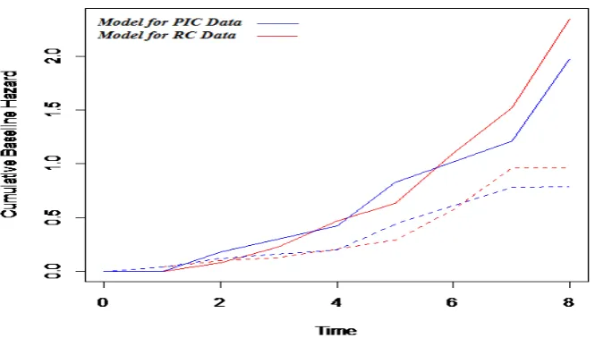
β1 1.009 1.002 0.486 (0.0658, 1.973) 0.7739 0.7677 0.473 (-0.1436 , 1.730)
β2 0.7331 0.719 0.667 (-0.05647, 2.072) 0.5075 0.4995 0.6436 (-0.7413 , 1.803)
*Posterior credible interval.
Solid line=cause1, Dashed line=cause2
Figure1: Comparison of cumulative baseline hazards from the two approaches.
5. Illustration
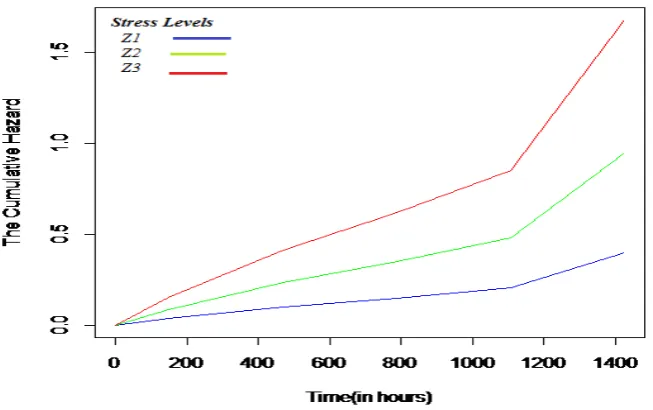
causes have almost equal cumulative hazard. In addition, figure 3-5 demonstrates that as stress increases the hazard increases, irrespective of cause. This is exactly the purpose of such experiments as it is run in high levels of stress to accelerate the failure and so reduce the cost and the experiment period.
Table 2: Number of units across masking sets and failure/censored times.
Failure time type
Masking sets
{0}** { T} { P} {G } {T,P } {T,G } {P,G } {T,P,G}* Total
Exact 0 0 0 1 0 1 0 0 2
Interval - 7 4 6 6 4 3 11 41
Left - 3 0 0 1 1 1 1 7
Right 10 - - - - 10
Total 10 10 4 7 7 6 4 12 60
*T=Turn, P=Phase, G=Ground. **{0}=No cause of failure or right-censored.
Table 3: The posterior summaries of the regression coefficients. Parameters Mean Median SE 95% PCI
β0T -21.49 -21.32 6.744 (-35.33, -8.82)
β0P -18.94 -18.74 7.739 (-34.82, -4.355)
β0G -20.96 -20.83 7.424 (-36.11, -6.728)
β1T 28.67 28.39 13.71 (2.698, 56.70)
β1P 22.55 22.17 15.75 (-7.589, 54.51)
β1G 27.09 26.88 15.10 (-1.971, 57.73)
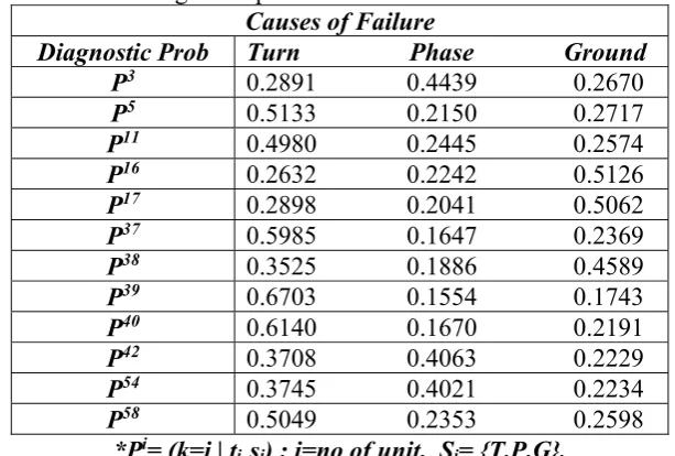
Table 4: Diagnostic probabilities of the full masked units. Causes of Failure
Diagnostic Prob Turn Phase Ground P3 0.2891 0.4439 0.2670
P5 0.5133 0.2150 0.2717
P11 0.4980 0.2445 0.2574
P16 0.2632 0.2242 0.5126
P17 0.2898 0.2041 0.5062
P37 0.5985 0.1647 0.2369
P38 0.3525 0.1886 0.4589
P39 0.6703 0.1554 0.1743
P40 0.6140 0.1670 0.2191
P42 0.3708 0.4063 0.2229
P54 0.3745 0.4021 0.2234
P58 0.5049 0.2353 0.2598
*Pi= (k=j | t
Figure 2: Cumulative baseline hazard of the three causes.
Figure 3: Cumulative hazard of cause turn.
Figure 5: Cumulative hazard of cause ground.
6. Conclusion
In this study, Bayesian analysis for competing-risk models was derived from conditions of masked failure cause and incomplete failure time. This method offers some flexibility in modeling as it is not built on assumptions with questionable validity such as the symmetry assumption or independence of the competing risks. Furthermore, it provides an assessment of the risk factors’ (covariates) effect on the hazard function. Based on the simulation results, it can be seen that our method is feasible.
Acknowledgments
The authors would like to thank Mrs Lynn Mason for editing the manuscript language. References
Basu, S., Asit, P.B. & Mukhopadhyay, C., 1999. Bayesian analysis for masked system failure data using non-identical Weibull models. Journal of Statistical Planning and Inference, 78, pp.255–275.
Basu, S., Sen, A. & Banerjee, M., 2003. Bayesian analysis of competing risks with partially masked cause of failure. Journal of the Royal Statistical Society: Series C (Applied Statistics), 52(1), pp.77–93. Available at: http://doi.wiley.com/10.1111/1467-9876.00390. Beyersmann, J. et al., 2009. Simulating competing risks data in survival analysis. Statistics in
Medicine, 28(6), pp.956–971. Available at: http://doi.wiley.com/10.1002/sim.3516.
Craiu, R. V & Reiser, B., 2006. Inference for the dependent competing risks model with masked causes of failure. Lifetime data analysis, 12(1), pp.21–33. Available at:
http://www.ncbi.nlm.nih.gov/pubmed/16583297 [Accessed June 13, 2014].
Association, 81(394), pp.328–336.
Flehinger, B.J., Reiser, B. & Yashchin, E., 2002. Parametric modeling for survival with competing risks and masked failure causes. Lifetime data analysis, 8(2), pp.177–203. Available at: http://www.ncbi.nlm.nih.gov/pubmed/12048866.
Guttman, I., Lin, D .K.J., Reiser, B., and Usher, J. S., 1994. Dependent masking and system life data analysis: Bayesian inference for two-component systems. Lifetime Data Analysis, 1(1), pp.87–100. Available at: http://link.springer.com/10.1007/BF00985260 [Accessed April 23, 2014].
Han, L., Gao, Q., Yang, J., Wu, Q., Zhu, B., Zhang, H., Ding, B., and Ni, C., 2017. Survival Analysis of Coal Workers ’ Pneumoconiosis ( CWP ) Patients in a State-Owned Mine in the East of China from 1963 to 2014. Int. J. Environ. Res. Public Health, 14(5).
Klein, J.P. & Basu, A.P., 1981. Weibull Accelerated Life Tests When There are Competing Causes of Failure.
Kuo, L. & Yang, T.Y., 2000. Bayesian reliability modeling for masked system lifetime data. Statistics & Probability Letters, 47(3), pp.229–241. Available at:
http://linkinghub.elsevier.com/retrieve/pii/S0167715299001601.
Liu, S., Huang, L., Chung, W., Chang, H., Wu, J., Chen, L., Chen, Y., Huang, W., Chang, H., and Lo, S., 2017. Increased Risk of Stroke in Patients of Concussion : A Nationwide Cohort Study. Int. J. Environ. Res. Public Health, 14(3).
Lu, K. & Tsiatis, A.A., 2001. Multiple imputation methods for estimating regression coefficients in the competing risks model with missing cause of failure. Biometrics, 57(4), pp.1191–7. Available at: http://www.ncbi.nlm.nih.gov/pubmed/11764260.
Martin J. Crowder, 2001. Classical Competing Risks, Chapman& Hall/CRC.
Miyakawa, M., 1984. Analysis of Incomplete Data in Competing Risks Model. IEEE Transactions on Reliability, R-33(4), pp.293–296. Available at:
http://ieeexplore.ieee.org/lpdocs/epic03/wrapper.htm?arnumber=5221828 [Accessed July 2, 2014].
Mukhopadhyay, C. & Basu, A.P., 1997. Bayesian analysis of incomplete time and cause of failure data. Journal of Statistical Planning and Inference, 59(1), pp.79–100. Available at: http://linkinghub.elsevier.com/retrieve/pii/S0378375896001036 [Accessed April 23, 2014]. Mukhopadhyay, C. & Basu, S., 2007. Bayesian Analysis of Masked Series System Lifetime
Data. Communications in Statistics - Theory and Methods, 36(2), pp.329–348. Available at: http://www.tandfonline.com/doi/abs/10.1080/03610920600853357 [Accessed June 13, 2014].
Neath, A. a. & Samaniego, F.J., 1996. On bayesian estimation of the multiple decrement function in the competing risks problem. Statistics & Probability Letters, 31(2), pp.75–83. Available at: http://linkinghub.elsevier.com/retrieve/pii/S0167715296000168.
Reiser, A.B. et al., 1995. Bayesian Inference for Masked System Lifetime Data. , 44(1), pp.79– 90.
Sen, A., Banerjee, M., Li, Y., and Noone, M., 2010. A Bayesian approach to competing risks analysis with masked cause of death. Statistics in medicine, 29(16), pp.1681–95. Available at: http://www.ncbi.nlm.nih.gov/pubmed/20575048 [Accessed March 23, 2014].