Optimizing the operating time of wireless sensor network

(1)

R E S E A R C H

Open Access

Optimizing the operating time of wireless sensor

network

Thanh Tung Nguyen

1*

and Van Duc Nguyen

2

Abstract

A difficult constraint in the design of wireless sensor networks (WSNs) is the limited energy resource of the batteries of the sensors. This limited resource restricts the operating time that WSNs can function in their applications. Routing protocols play a major part in the energy efficiency of WSNs because data communication dissipates most of the energy resource of the networks. There are many energy-efficient cluster-based routing protocols to deliver data from sensors to a base station. All of these cluster-based algorithms are heuristic. The significant benefit of heuristic algorithms is that they are usually very simple and can be utilized for the optimization of large sensor networks. However, heuristic algorithms do not guarantee optimal solutions. This article presents an analytical model to achieve the optimal solutions for the cluster-based routing protocols in WSNs.

Keywords:Sensor networks, Routing, Cluster networks, Battery, Linear programming, Optimization.

Introduction

There is a common problem in energy efficiency consid-erations in wireless sensor networks (WSNs): maximiz-ing the amount of data sent from all sensor nodes to the base station (BS) until the first sensor node is out of bat-tery. In sensor networks, sensors send data to each BS periodically during each fixed amount of time. Thus, the problem is the same as maximizing network operation lifetime until the first sensor node run out of battery. Numerous studies have been done on the energy effi-ciency using cluster-based routing in WSNs [1-5]. Cluster-based routing was originally used to solve the scalability problems and resources-efficient communica-tion problems in wire-line and wireless networks [6,7]. The method can also be used to perform energy-efficient routing in WSNs. In the cluster-based routing, nodes cooperate to send sensing data to a BS. In this routing, a network is organized into clusters and nodes play different roles in the network. A node with higher remaining energy can be elected as the cluster head (CH) of each cluster. This node is responsible to receive data from its members in the cluster and to send the data to the BS.

However, all of the above-mentioned cluster-based routing work is heuristic. The real benefit of heuristic algorithms is that they are usually very simple and can be used for the optimization of large sensor networks. However, in general, heuristic algorithms do not guaran-tee optimal solutions.

In this article, an analytical model is used to obtain the optimal solutions for the above clustering lifetime prob-lem. The basic idea is to formulate the problem as an integer linear programming (ILP) problem and to utilize ILP solvers [8] to compute the optimal solutions. These solutions are employed to evaluate the performance of previous heuristic algorithms. These analytical models are used to formulate the system lifetime problem into a simpler problem, find the optimum solution for the sys-tem lifetime problem, and evaluate the performance of heuristic models.

This article is organized as follow. The following sec-tion summarizes previous work in energy efficiency using cluster-based routing. Then, an analytical model of the cluster-based routing is developed. The model is first implemented by an analysis of a simple network with one cluster. After that, the analysis is extended for more complex cases of multiple clusters. A new heuristic cluster-based routing is also proposed. Finally, the simu-lation results of the analytical model, old heuristic solu-tions, and the new ones are presented and discussed.

* Correspondence:[email protected] 1

International School, Vietnam National University, 144 Xuan Thuy, Cau Giay, Hanoi, Vietnam

Full list of author information is available at the end of the article

(2)

Previous work in energy efficiency using cluster-based routing

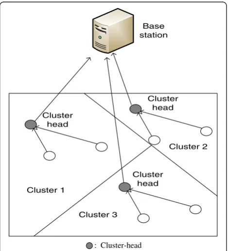
In a cluster-based routing, higher remaining energy nodes can gather data from low ones, perform data ag-gregation, and send the data to a BS. Nodes in networks are grouped into clusters, and nodes that have higher remaining energy are elected as the CHs. In each cluster, the nominated CH node receives and aggregates data from all sensor nodes in the cluster. Usually, the sizes of the data of all sensors are the same and the aggregated data at the CH node has the same size with the data of every sensor in the cluster. As the data are aggregated in the CH node before reaching a BS, this technique reduces the amount of information sent to the distant BS, hence saves energy. For example, if each sensor in the cluster sends a message of 100 bits to the CH node, then the CH node sends the aggregated message of 100 bits to the BS. Details are given in [2,6,9]. As shown in Figure 1, all nodes in Cluster 1 send data to the CH. The node aggregates the data with its own data and sends the final data to the BS.

In sensor applications, every sensor node sends data periodically to its BS. Initially, every node starts with the initialized battery storage. A round of data transmission is defined as the duration of time to send a unit of data to the BS. At the end of each round, every sensor node loses an amount of energy which is used to send a unit of data to the BS. The lifetime of sensor networks is

defined as the total number of rounds sending data to the BS until the first node is off.

Heinzelman et al. [1,2] proposed a Low-Energy Adap-tive Clustering Hierarchy (LEACH). In LEACH, the op-eration of the protocol is divided into rounds. Each round consists of the setup and the transmission phase. In the setup phase, the network is divided into clusters and nodes negotiate to nominate CHs for the round. In more details, during the setup phase, a predetermined fraction of nodes, p, elect themselves as CHs as follows. A node picks a random number,r, between 0 and 1.

If(r<T(n))then

The node becomes a CH for the current round else

The node remains a non-CH node whereTis a threshold value given by:

T nð Þ ¼p:n∈G; ð1Þ

whereGis the set of nodes that are involved in the CH election. The selected CHs for the round advertise them-selves as the round’s new CHs to the rest of the nodes in the network. All the non-CH nodes decide on the clus-ter to which they want to belong to. The decision is based on the distance to the closest CH.

In the transmission phase of LEACH, the elected CH collects all the data from nodes in its cluster, aggregates these data, and forwards them to a BS. In the next rounds, the process is repeated and CH positions are reallocated among all nodes in the network to extend the network lifetime.

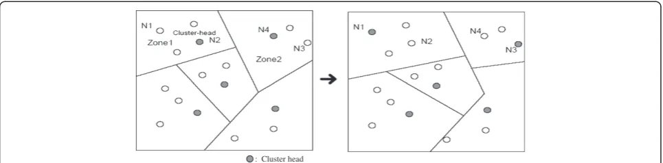
For examples, as can be seen from Figure 2, the role of CH for Zone 1 is moved from Node 2 to Node 1 and the role of CH for Zone 2 is moved from Node 4 to Node 3 in the next round of data transmission. There-fore, the energy dissipation of these nodes during the network operation is balanced.

The LEACH protocol ensures that every node can be-come a CH exactly once within 1/p rounds. This will not give the optimum network lifetime, as sensor nodes that are far away from the BS will consume more energy than closer nodes to send data to the BS. Therefore, nodes, which are close to BS, need to become CHs more frequently than other nodes.

There are some LEACH variants to address the above issues in LEACH protocol [3,10-13]. Saha Misra et al. [3] proposed the energy enhanced-efficient adaptive clustering protocol for distributed sensor networks. CHs can be formed based on the residual energy of each node. The residual energy is calculated for every node after each round of transmission. Every node transmits a code containing the information about its residual Cluster 1

(3)

energy and its identification. If this residual energy is more than the ones of all other nodes in the same sub-area, then the node is the CH for that round in this sub-area. Otherwise, it can detect the node that has the maximum residual energy and elects this node as the CH.

A different approach was used by the authors of [4,5] who add the current energy information of sensor nodes into Equation (1).

T nð Þ ¼ p

1p rð mod 1ð =pÞÞ Ecurrent

Einitial ;

n∈G; ð2Þ

whereEcurrentis the current energy of Node nandEinitial

is the initial energy of the node.

If (r<T(n)) then

The node becomes a CH for the current round else

The node remains a non-CH node

Simulation results showed that the lifetime of the network with the scheme is improved 30% compared with the LEACH algorithm under the same experiments for LEACH.

After the design of LEACH protocol, these authors fur-ther proposed a new centralized version called LEACH_C in [2]. Unlike LEACH, LEACH_C utilizes the BS for creat-ing clusters. Durcreat-ing the setup phase, the BS receives the information about the location and the energy level of each node in the network. Using this information, the BS decides the number of CHs and configures the network into clusters. To accomplish this, the BS computes the average energy of nodes in the network, and nodes that have energy storage below this average cannot become CHs for the next round. From the remaining CH nodes, the BS uses the simulated annealing (SA) algorithm to find thekoptimal CHs. The selection problem is an NP-hard problem [14,15]. The solution attempts to minimize the total energy required for non-CH nodes in sending data to the corresponding CHs. As soon as the CHs are found, the BS broadcasts a message that contains a list of CHs

for all sensors. If a node CH’s ID matches its own ID, the node becomes a CH. Otherwise, the node determines its TDMA slot for its data transmission from the broadcast message and turns off its radio until the transmission phase. The transmission phase of LEACH_C is identical to that of LEACH. Under the same experimental settings, LEACH_C improves LEACH from 30 to 40%.

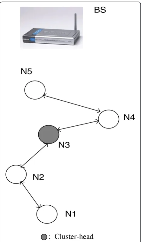
Besides cluster-based routings [10-13], there is also a chain-based one. Lindsey and Raghavendra [16] pro-posed one type of chain-based protocol called power-efficient gathering in sensor information systems (PEGASIS), which is near optimal for gathering data in sensor networks. PEGASIS forms a chain among sensor nodes so that each node will receive data from a near neighboring node and transmit data to another near neighbor. Gathered data move from a sensor node to the nearest neighbor, are aggregated with the neighbor’s data, and eventually reach a determined CH before fi-nally being transmitted to the BS. Figure 3 illustrates the ideas of the PEGASIS protocol. In this round of data transmission, Node 3 is elected as the CH. Node 5 trans-mits data to Node 4, and Node 4 fuses the data with its own data and transmits the fused data to Node 3. Simi-larly, Node 1 transmits data to Node 2, and Node 2 transmits the fused data to Node 3. Finally, Node 3 fuses the data of the other nodes with its own data and trans-mits the final fused data to the BS. The data fusion func-tion can be any funcfunc-tion, e.g., minima, maxima, and average, depending on specific applications. Nodes take turns equally to be the CH so that the energy spent by each node is balanced. In other words, each node becomes a CH once for everynrounds of data transmis-sion, wherenis the number of sensor nodes.

The comparison between the chain-based routings and cluster-based routings were done extensively in [9] and this is not mentioned here as this article only fo-cuses on cluster-based routing.

In the next section, an analytical model is presented to achieve the optimal solutions for the frequency of CHs of sensor nodes. The basic idea is to formulate the prob-lem as an ILP probprob-lem and to utilize ILP solvers [8] to : Cluster head

(4)

compute the optimal solutions. These solutions are employed to evaluate the performance of previous heur-istic algorithms.

Analytical model for optimizing the lifetime of sensor network with one CH

In order to minimize the complexities of the clustering problem, the wireless radio energy dissipation model

is not used. This assumption does not change the validation of any simulation result. A very simple energy usage model is given as

E(S) =αd2,E(D) = 0, forα> 0

whereSdenotes a source node,Ddenotes a destination node, E(S) is the energy usage of node S, and dis the distance from Sto D. This formula states that the en-ergy required to transmit a unit of data is proportional to the square of the distance to a destination, and there is no energy spent at the destination. In this section,α is set to 1.

Let us analyze a very simple network to establish a general method that can be applied for any complicated problem. Figure 4 shows a simple network topology in which there are five nodes that lie on a line. The nodes are located equally from position 0 to position 80 m and the BS is located on the position 175 m. In sensor appli-cations, every sensor node sends data periodically to the BS. A round of data transmission is defined as the dur-ation of time to send a unit of data to the BS. Therefore, the lifetime of sensor networks is defined as the total number of rounds of sending data to the BS until the first node is off. It is assumed that every node starts with the equal initial battery storage of 500,000 units. The problem is maximizing the total the number of rounds of sending data to the BS until the first sensor node runs out of battery.

In each round of operation, every node must transmit a unit of data to the BS. It is also assumed that only one node acts as the CH in each round of transmission and the role is reallocated among all nodes so the system lifetime is maximized. The analytical model needs to compute the optimal usage of nodes as CHs under the battery constraint of every sensor.

Let us denote xj, ∀j∈ [1. . .5] to be the number of

rounds, which Node j becomes a CH and cjibe the

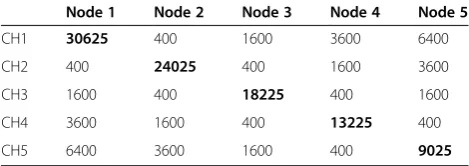
en-ergy consumption of Node i, to deliver a unit of data in each round, when Nodejbecomes a CH,∀i,j∈ [1. . .5]. As there are five nodes and only one CH, there are five possible choices for the CH in each round and there are also five energy usages for these five sensor nodes, re-spectively. This is shown in Table 1. For example, the energy dissipation of Node 1 when Node 5 becomes a

N1

N2

N4

N5

N3

BS

: Cluster-head

Figure 3A reconstructed chain from PEGASIS method.

Base station

N1 N2 N3 N4 N5

0 m 20 m 40m 60m 80m

175m

(5)

CH, c51 is (80 – 0)2 = 6400, the energy dissipation of

Node 1 when Node 1 becomes a CH,c11is (175–0)2=

30625. The optimum number of transmission rounds (or system lifetime) for the network is written as the follow-ing ILP problem.

whereEiis the initial battery storage of nodei.

Formula-tion (3) states that the total number of rounds must sat-isfy the battery storage constraint of every sensor node.

Table 2 shows the optimum result obtained from (3) when the battery capacity increases from 125,000 to 50 million units. When the battery size is large enough (greater than 1 million units), the number of rounds that each node becomes a CH increases almost linearly with the battery capacity (e.g., the number of rounds of each node is nearly doubled when the battery capacity is increased from 1 to 2 million).

Simplification of formulation (3)

Formulation (3) can be converted to a linear program-ming (LP) formulation as given below:

Maximize:X

where the condition of variables being integers is removed. There are two cases to use the formulation to obtain the optimization solutions:

(1)Ei→∞then the solution of (4) becomes the

solution of (3)

(2)Ei≠∞then the solution of (4) is the approximation of the solution of (3)

Formulation (4) can remove the NP-hard characteristic of the ILP formulation (3). Therefore, the optimization solution can be solved by the simplex method [8,9]. In the next section, we will verify the solutions obtained from both formulations. A simple network topology of 11 nodes is given in Figure 5. All nodes are located equally on the line. The nodes are located equally from position 0 to position 100 m (separated each 10 m) and the BS is located on the position 175 m.

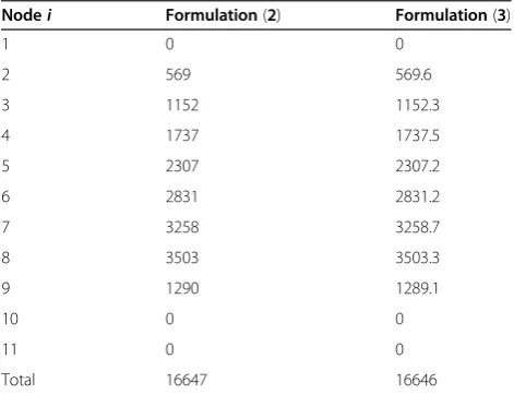
In the simulation, each node starts with an equal amount of initial energy of 500 million units. The life-time problem for the network is first formulated as an ILP problem using (3). Then the LP formulation as in (4) is used to calculate the approximate solutions. Table 3 shows that the solutions given by both methods are al-most identical. Therefore, the formulation of (4) can be an approximating solution of (3). Also, Nodes 10 and 11 never become a CH as they are too far from other nodes. Node 1 will never become a CH as it is too far from the BS.

Analytical model for optimizing the lifetime of sensor network with multiple CH

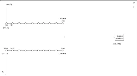
The previous section assumes a very simple case when there is only one CH. It is obvious that for the simple network of Figure 4, too many CHs will drain the energy of all sensor nodes very quickly as the nodes have to send data to the distant BS. This is not true for the other network topologies. The network considered in the ana-lysis section has 20 nodes. The network topology is given in Figure 6. All nodes are located equally on the two lines.

For the network, one CH could not be enough, as other non-CH nodes would consume energy significantly to deliver a unit of data to the CH in each round. Table 4 shows the performance of the network with a variable number of clusters. The simulation result shows that two CHs will minimize the total energy consumption to send data to the BS.

Table 1 The energy dissipatedc_ji(units) per round of

nodeiwhen nodejbecomes a CH

Node 1 Node 2 Node 3 Node 4 Node 5

CH1 30625 400 1600 3600 6400

CH2 400 24025 400 1600 3600

CH3 1600 400 18225 400 1600

CH4 3600 1600 400 13225 400

CH5 6400 3600 1600 400 9025

Table 2 The number of rounds that each nodeiis a CH

over the number of initial batteryE(units) of each node

E Node 1 Node 2 Node 3 Node 4 Node 5

125,000 0 2 5 8 11

250,000 0 5 11 17 13

500,000 1 11 22 34 44

1000,000 3 23 44 68 88

2000,000 7 46 89 135 176

(6)

When the number of CHs is more than one, it is much more complicated to obtain optimum solutions. The number of possible combinations of CHs isO(nk), where nis the number of sensor nodes andkis the number of CHs. Furthermore, with a selected solution of CHs, each sensor has k choices to select its CH. Therefore, the method of finding the optimum solution includes two optimization processes: optimization of the position of CHs and optimization of gathering traffic to the CHs.

In order to design an analytical model for complex cases with multiple CH in sensor networks, Theorem 1 is stated and proved.

Theorem 1:Consider two ILP problems with the same

objective function and the same variables, if the set of coefficients of ILP problem 2 is smaller than the set of coefficients of ILP problem 1, respectively, for all of these coefficients, then the optimal solution of Problem 2 is higher than that of Problem 1.

Consider two ILP problems:

Problem 1:

Maximize:X

n

j¼1 xj

Subject to:

Xn

j¼1

ci_jxj≤Ei:∀i∈½1. . .mxj∈Zþ:∀j∈½1. . .n ð5Þ

Problem 2:

Maximize:X

n

j¼1

xj

Subject to:

Xn

j¼1

c0_jixj≤Ei:∀i∈½1. . .mxj∈Zþ:∀j∈½1. . .n ð6Þ

Definition:O1is the optimal solution of Problem (5).

O2is the optimal solution of Problem (6)

Ifc'ji≤cji∀i∈[1. . .m],∀j∈[1. . .n],thenO2≥O1

Proof: Sincec'ji≤cji∀i∈[1. . .m],∀j∈[1. . .n] andO1is the

optimal solution of Problem 1, thenO1is a feasible solution

of Problem 2 becauseO1satisfy all constraints of (6). Since

O2is the optimal solution of Problem 2,O2≥O1■

To illustrate Theorem 1, let us consider two simple ILP problems:

Simple problem 1:

Maximizex1+x2

Subject to:

2x1þ3x2≤20 3x1þ4x2≤20

x1;x2∈Zþ ð7Þ

Simple problem 2:

Maximizex1+x2

Subject to:

x1þ2:5x2≤20 2:5x1þ3:5x2≤20

x1;x2∈Zþ ð8Þ

Applying Theorem 1 for two simple problems (1) and (2), as the coefficients of the constraint functions (7) are all higher than those of (8) respectively, the optimal solution

Base station

N1 N2 N3 N4 N5

0 m 10 m 20m 30m 40m

175m

N6 N7 N8 N9 N10

50 m 60 m 70m 80m 90m N11

100m

Figure 5A simple topology of 11 nodes on a line.

Table 3 The number of rounds each nodeibecomes a CH

solved by formulations (2) and (3)

Nodei Formulation(2) Formulation(3)

1 0 0

2 569 569.6

3 1152 1152.3

4 1737 1737.5

5 2307 2307.2

6 2831 2831.2

7 3258 3258.7

8 3503 3503.3

9 1290 1289.1

10 0 0

11 0 0

(7)

of (7) must be smaller than that of (8). This result is verified by using the ILP solver in [8]. The optimal solution of Simple problem (1) is 6 while the optimal solution of Simple problem (2) is 8.

This theorem is important because in many cases, this is very hard to calculateO1. One of the reasons is that

work-ing out all coefficientscjiis impossible. Based on the theory,

we know thatO2can be an upper bound ofO1, or all the

feasible solutions of Problem 1 are bounded byO2.

Theorem 2:Given a clustering sensor network with k

CHs, connection from non-CH nodes to the closest CH node of the kCHs provides the optimal lifetime for the clustering network.

In more detail, we are given a set ofnsensors located in two-dimensional space R2. Let us define S as the set of ways to select kCHs in the given set ofn sensors. If every CH is different to the remaining k − 1 CHs, the

number of elements in Sis n

k . However, in the the-orem, some CHs might be the same and these same CHs are considered as one CH. Therefore, the number of elements inSisnkelements. Let us definesnk(i) as the

ith element in S wherei in (1. . .nk). Let us define cij as

the energy usage of Node j consumes, when the ith element in S is selected as the CHs. Let us define nias

the number of rounds, which the ith element in S is selected as the CHs. Let us defineEjas the initial energy

of NodejandOas the optimal solution of the following ILP problem:

Maximize:

Xnk

i¼1

ni ð9Þ

Subject to:

Xnk

i¼1

nicji≤Ej:∀j∈½1. . .nni∈Zþ:∀i∈ 1. . .nk

The energy cij is equal to the energy dissipation of

Node jto send a unit of data to the closest sensor node in the ith element in S. Then,O is the optimal lifetime for the sensor network withkCHs.

Proof: Let us denote c0ij as the energy usage in any

arbitrary way to send a unit of data from sensor node j to the ith element in S, ∀i∈S, ∀j∈[1. . .n]. The optimum selection of CHs ofSis found by solving the mixed integer programming (MIP) problem below:

Base station

(50,175)

(70,90) (70,0)

(30,0)

N1 N2

N11 N12

N10

N20 (30,90) (0,0)

X

Y

Figure 6A simple network topology of 20 nodes on 2 lines,where each line has 10 nodes.The BS is at (50, 175).

Table 4 The average energy dissipated (units) per round over the number of CHs

1 CH 2 CHs 3 CHs

(8)

Maximize:

Xnk

i¼1

ni ð10Þ

Subject to:

Xnk

i¼1

nic0ij≤Ej:∀j∈½1. . .n ni∈Zþ:∀i∈ 1. . .nk

Asc'ij≥cij∀i∈S,∀j∈[1. . .n], since cijis equal to the

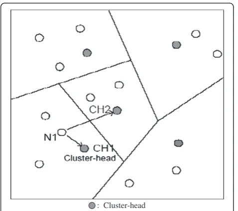
en-ergy dissipation of Node jto send a unit of data to the closest sensor node in theith element inS, any optimum solution O’of (10) is smaller than the optimum solution Oobtained by (9) as Theorem 1. This statement is illu-strated in Figure 7. As the result, O is the global optimum solution for maximizing the operation time withkCHs.■

Calculation of coefficients for Problem (9)

The energy coefficientscijof formulation (9) for a network

ofnnodes withkCHs can be calculated as follows:

Forevery combination ofkCHs from thennodes Forevery node from thennodes

If(the node is a CH)then

cj_i¼d2_toBS

else

cj_i¼d2_toCH

End of code

where dtoCH is the distance from the sensor node to

the closest CH from the k CHs, dtoBS is the distance

from the sensor node to the BS.

Figure 8 shows that for the current selection ofk= 3 CHs and n= 15 nodes, the energy coefficient of Node 2 is equal to d242, and the energy coefficient of Node 1 is

equal tod12.

Theorem 3: The problem formulation in (9) provides

the optimum solution for maximizing the operation time for any clustering network with the number of CHs smaller than or equal tok.

Proof:As stated in Theorem 2,S is the set of ways to select k CHs in the given set of n sensors. In each

: Cluster-head

Figure 7Connection from Node 1 to any CH will dissipate more energy than connection to CH 1 (the closest CH of Node 1).

: Cluster-head

Figure 8Calculation of energy coefficients for a network of 15 nodes with 3 CHs.

Table 5 The average energy dissipated (units) per round and the number of rounds over the number of CHs

1 CH 2 CHs 3 CHs

Energy per round (units) 65933 62016 69560

(9)

combination selection, some CHs might be identical and these identical CHs are considered as one CH. In this case, the number of CHs is less than k. Therefore, any network of less than k CHs is a special element in S, where some CHs are the same.■

It is of interest to know the optimum solution of the network topology in Figure 6. Every sensor node begins with 1 million units of energy and the above-mentioned simple energy model is used. Table 5 shows the optimum system lifetime versus the number of CHs. The results show that the network achieves the optimum solution at the number of two CHs.

It is also of interest to see the distribution of opti-mums CHs among the 20 sensor nodes in Figure 6. The distribution depends on the position of sensors. The en-ergy model used isd2energy model (gamma = 2).

Figure 9 shows the five pairs that are chosen as CHs most frequently. The results show that the pair of nodes (7, 17) is the most preferred CHs. This is due to the fact that the nodes are not very far from the BS as well as the rest of other nodes. As such, they can become inter-mediate CHs to deliver data to the BS. The five pairs are selected as CHs for 56% of the total number of rounds.

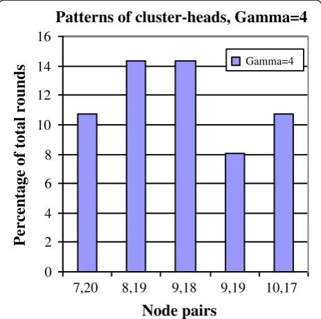
The same experiments are carried out on the same network over the “power 4” (gamma = 4) model. The model is given below:

E(S) =αd4,E(D) = 0, forα> 0

where S denotes a source node, Ddenotes a destination node,E(S) is the energy usage of nodeS, anddis the dis-tance from S to D. This formula states that the energy required to transmit a unit of data is proportional to the

“power 4” of the distance to a destination, and there is no energy spent at the destination. For the rest of this section,αis set to 1.

Figure 10 shows the simulation results whenαis set to 1. Compared to the previous results, the CHs move closer to the BS. This is because when the “power 4” model is used, the energy of CH nodes is drained quickly. As such, the nodes need to be closer to the BS. The five pairs are selected as CHs for 58% of the total number of rounds.

A simplified LEACH_C protocol (AVERA)

As mentioned in the Section “Previous work in energy efficiency using cluster-based routing”, LEACH_C uti-lizes the BS for creating clusters. During the setup phase, the BS receives information about the location and the energy level of each node in the network. Using this in-formation, the BS decides the number of CHs and con-figures the network into clusters. To do so, the BS computes the average energy of nodes in the network. Nodes that have energy storage below this average can-not become CHs for the next round. From the remaining possible CH nodes, the BS uses the SA algo-rithm to find thekoptimal CHs. The selection problem is an NP-hard problem.

If the BS is also far away from main power sources and is energy-limited and processing-limited, it is im-practical for the BS to run LEACH_C as it creates sig-nificant delay and requires sigsig-nificant computation. In this case, we modify LEACH_C algorithm by removing

Patterns of cluster-heads, Gamma=2

0

4,19 6,18 7,17 8,16 9,14

Node pairs

Percentage of total rounds

Gamma=2

Figure 9Percentage of the total number of rounds that each pair of nodes is a pair of CHs ford2_{energy model.}

Patterns of cluster-heads, Gamma=4

7,20 8,19 9,18 9,19 10,17

Node pairs

Percentage of total rounds

Gamma=4

(10)

the SA algorithm process. In more details, our algorithm AVERA is implemented as below.

AVERA:

In every round, select k CHs randomly from m sensor nodes that have their energy level above the average en-ergy of all nodes.

Given:

N: The number of sensor nodes indexed from 1 toN s: The current CH solution

m: The number of sensor nodes that have energy above the average energy of all sensors

Forevery round of data transmission s=k sensors in Random[1. . .m]

Result: s is the CH solution for the round obtained

from the AVERA algorithm. (End of code)

Simulation and comparison

Most of previous work on WSN lifetime [1-5] used the energy consumption model and the energy dissipation parameters given in [9]. The data are kept the same in our experiments to make the comparison between our proposed algorithms and previous ones feasible. The power transmission coefficients for free space and multi-path are given below.

εFS¼10pJ=b=m2

εMP¼:0013pJ=b=m4

From the parameters, the output power of a transmit-ter over a distancedis given by

Pampð Þ ¼d

experiments in [1,2,17-19] and is set to 50 nJ/bit.

In summary, the total transmission energy of a mes-sage ofkbits in sensor networks is calculated by

Et=kEelec+εFSkd2, whend<do

Et=kEelec+εMPkd4, whend>do

and the reception energy is calculated by

Er¼Eeleck

whereEelec,εFS,εMP, anddoare given above.

First, the optimum number of CHs of these networks is studied. In the experiments, 100 random 80-node sensor networks are generated. Each node begins with 1 J of en-ergy. The network settings for the simulations are given

below. The sensor positions and the BS position are defined as below . This is the same settings used in [1-5,9,18,19].

Network size (100m× 100m) Base station (50m, 175m)

Number of sensor nodes 100 nodes Data message size: 4000 bits Broadcast message: 200 bits Energy message: 20 bits

Position of sensor nodes: Uniform placed in the area Energy model: Eelec =50* 10−9 J, εfs =10* 10−12 J/bit/

m2andεmp=0.0013* 10−12J/bit/m4

During the sensor operation, every sensor node sends data periodically to the BS. A round of data transmission is defined as the duration of time to send a unit of data (4000 bits) to the BS. Each round consists of a setup and a transmission phase. In the setup phase, the network is divided into clusters and nodes negotiate to nominate CHs for the round. In the LEACH_C and AVERA proto-cols, each node sends its energy level message to the BS (20 bits). The BS decides the CHs for the round and sends a broadcast message (200 bits) about the decision for the round to all sensor networks.

In the transmission phase, the elected CH collects all data from nodes in its cluster and forwards the data to a BS. After each round, every sensor node loses an

Figure 11Average energy dissipation per round(units)over the number of CHs.

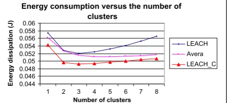
Energy consumption versus the number of clusters

(11)

amount of energy for the data transmission in the round. The amount depends on the distance from the sensor to its CH or to the BS. The lifetime of sensor networks is measured as the total number of rounds sending data to the BS until the first node is off.

LEACH, LEACH_C, and AVERA are used over 100 network topologies while varying the number of CHs from 1 to 8, and the system lifetime and the energy dis-sipation per round are recorded for these numbers of CHs.

Figure 11 shows that the energy dissipation per round is minimized for LEACH, LEACH_C, and AVERA at the number of CHs from 3 to 4. The result agrees well with the analytical model and the results are presented in [1,2,17].

Validation of the analytical model

In this section, the performance of LEACH, LEACH_C, and AVERA and the optimum solution from the analyt-ical model is verified. The number of CHs is set to three in all methods. All methods are run over the above 100 random 80-node network topologies and the ratio be-tween the lifetime of the three protocols and the optimum are recorded. For the calculation of the optimum solution, we use the GNU Linear Programming Kit (GLPK) and the MIP solver. GLPK is a free GNU LP software package for solving large-scale LP, MIP [8].

GLPK provides two methods to solve LP and MIP problems:

(1) Create a problem in C programming language that calls GLPK API routines

(2) Create a problem in a text editor and use a standalone LP/MIP solver to solve it.

We use method 2 to calculate the optimum solution. Figure 12 shows that both AVERA and LEACH_C per-form very closely to the optimum solution while LEACH is only 70% of the optimum solution.

The computation time for all three protocols is also recorded on the 100 network topologies. The computa-tional time for LEACH, AVERA, and LEACH_C are 1.6,2.5, and173.2 s, respectively. This shows that the new protocol AVERA provides a reasonably good operation time while guarantees less processing from the BS.

Conclusion

This article has presented some energy-efficient cluster-based routing protocols. In sensor networks, BSs only require a summary of the events occurring in their en-vironment, rather than the sensor node’s individual data. To exploit the function of the sensor networks, sensor nodes are grouped into small clusters so that CH nodes can collect the data of all nodes in their cluster and

perform aggregation into a single message before send-ing the message to the BS. Since all sensor nodes are en-ergy-limited, CH positions should be reallocated among all nodes in the network to extend the network lifetime. The determination of adaptive clusters is not an easy problem. We start by analyzing simple networks with one CH first to be able to obtain an effective solution for the problem. Then the model is extended to net-works with multiple CHs.

Heuristic algorithms are also proposed to solve the problem. Simulation results show that LEACH solution performs quite far from the optimum solution as it does not directly work on the remaining energy of all sensor nodes. At the same time, both AVERA and LEACH_C solutions perform very closely to the optimum solution. Note that the computational time for AVERA is also 1.4% of LEACH_C.

Competing interests

The authors declare that they have no competing interests.

Acknowledgment

This research is carried out under the frame work of the Project number 102.04-2012.35 funded by the Vietnamese National Foundation for Science and Technology Development (NAFOSTED).

Author details

1

International School, Vietnam National University, 144 Xuan Thuy, Cau Giay, Hanoi, Vietnam.2_{Faculty of Electronics and Telecommunications, Hanoi} University of Science and Technology, Dai Co Viet Str. 1, Hanoi, Vietnam.

Received: 13 September 2011 Accepted: 26 October 2012 Published: 21 November 2012

References

1. WB Heinzelman, AP Chandrakasan, H Balakrishnan, Energy-efficient communication protocol for wireless microsensor networks, in33rd Hawaii

International Conference Systems Sciences, 2000, p. 10. Vol.2. ISBN:

0-7695-0493-0

2. WB Heinzelman, AP Chandrakasan, H Balakrishnan, An application specific protocol architecture for wireless microsensor networks. IEEE Trans. Wirel. Commun1(4), 660–670 (2002)

3. I Saha Misra, S Dolui, A Das, Enhanced-efficient adaptive clustering protocol for distributed sensor networks, inIEEE ICON, 2005, p. 6. doi:10.1109/ ICON.2005.1635525. Vol.1, ISBN:1-4244-0000-7

4. J Zhang, B Huang, L Tu, F Zhang, A cluster-based energy-efficient scheme for sensor networks, inThe Sixth International Conference on Parallel and

Distributed Computing, Applications and Technologies (PDCAT’05), 2005, pp.

191–195. doi:10.1109/PDCAT.2005.3. ISBN: 0-7695-2405-2

5. R Chang, C Kuo, An energy efficient routing mechanism for wireless sensor networks, inThe 20th International Conference on Advanced Information

Networking and Applications (AINA’06), 2006. Vol.2, p. 5. doi:10.1109/

AINA.2006.86. ISSN: 1550-445X; ISBN: 0-7695-2466-4

6. JN Al-Karaki, AE Kamal, Routing techniques in wireless sensor networks: a survey. IEEE Wirel. Commun.11(6), 6–28 (2004)

7. J Deng, YS Han, W Heinzelman, Balanced-energy sleep scheduling scheme for high density cluster-based sensor networks. Comput. Commun.28, 1631–1642 (2005)

8. GLPK programming, 2011. http://www.gnu.org/software/glpk/ 9. T Nguyen Thanh,Energy-efficient routing algorithms in wireless sensor

networks. PhD thesis (Monash University, Australia, 2008)

10. L Guo, Y Xie, C Yang, Z Jing, Improvement on LEACH by combining adaptive cluster head election and two-hop transmission, in9th

International Conference on Machine Learning and Cybernetics, 2010, pp.

(12)

11. T Qiang, W Bingwen, W Zhicheng, MS-LEACH: a routing protocol combining multihop transmission and single-hop transmission, in

Pacific-Asia Conference on Circuits, Communications and Systems, 2009, pp. 107–110

12. M Farooq, AB Dogar, GA Shah, MR-LEACH: multi-hop routing with low energy adaptive clustering hierarchy, in4th International Conference on

Sensor Technologies and Applications, 2010, pp. 262–268

13. J Chen, H Shen, MELEACH-L: more energy efficient LEACH for large scale WSNs, inWireless Communications, Networking and Mobile Computing, 2008, pp. 1–4

14. SG Nash, A Sofer,Linear and Nonlinear Programming(McGraw-Hill, New York, 1996)

15. T Kanungo, DM Mount, NS Netanyahu, A local search approximation algorithm for k-means clustering, inThe Eighteenth Annual Symposium on

Computational geometry, 2002. Volume 28, Issues 2–3, pp. 89–112

16. S Lindsey, C Raghavendra, Power-efficient gathering in sensor information systems, inIEEE Aerospace Conference, 2002. Vol.3, p. 3-1125-3-1130. doi:10.1109/AERO.2002.1035242.0-7803-7231-X

17. WB Heinzelman,Application-specific protocol architectures for wireless

networks. PhD dissertation (Massachusetts Institute of Technology, 2000)

18. T Nguyen Thanh, V Phan Cong,The Energy-Aware Operational Time of

Wireless Ad-hoc Sensor Networks.ACM/Springer Mobile Networks and

Applications (MONET) Journal, Volume 17, August, 2012.

doi:10.1007/s11036-012-0403-1

19. T Nguyen Thanh,Heuristic Energy-Efficient Routing Solutions to Extend the

Lifetime of Wireless Ad-Hoc Sensor Networks(Springer, LNCS 7197, 2012), pp.

487–497. ISBN: 978-3-642-28489-2

doi:10.1186/1687-1499-2012-348

Cite this article as:Nguyen and Nguyen:Optimizing the operating time

of wireless sensor network.EURASIP Journal on Wireless Communications and Networking20122012:348.