R E S E A R C H
Open Access
A new Fibonacci type collocation procedure
for boundary value problems
Ay¸se Betül Koç
1*, Musa Çakmak
2, Aydın Kurnaz
1and Kemal Uslu
1*Correspondence:
[email protected] 1Department of Mathematics,
Faculty of Science, Selcuk University, Konya, Turkey
Full list of author information is available at the end of the article
Abstract
In this study, we present a new procedure for the numerical solution of boundary value problems. This approach is mainly founded on the Fibonacci polynomial expansions, the so-called pseudospectral methods with the collocation method. The applicability and effectiveness of our proposed approach is shown by some
illustrative examples. Then, the results indicate that this method is very effective and highly promising for linear differential equations defined on any subinterval of the real domain.
MSC: 35A25
Keywords: ordinary differential equations; spectral methods; collocation method; Fibonacci polynomials
1 Introduction
A lot of applications, which are of fundamental interest in numerical analysis, have been made on the expansion of an analytic functionf(x) in a series of the form
f(x) = ∞
k=
akϕk(x), (.)
where the set{ϕk(x)}is a special trial polynomial (or function) basis andak’s are constant
coefficients [–]. One of the main utilization areas of the expansions with different basis can be seen in the solution methods for the differential equations. The idea of finding the solution of a differential equation in form (.) goes back, at least, to Lanczos () [, ]. Then, three main techniques have been evolved from that idea, and each of these tech-niques has its own advantages in the implementation (details and applications of those can be seen in [–]). Here, we deal only with the pseudospectral (collocation) type method. In the pseudospectral method, the solution of a differential equation is expressed as a linear combination of the polynomials in the basis set. Therefore, the coefficients in the combination are determined by the use of certain discrete points calledcollocation points. Thus, the accuracy of the approximation and the efficiency of its implementation are closely related to the choice of the grid points and the basis set. Determination of an appropriate set of basis should be kept in view of some rules. The most common one of those rules is that the geometry or the field of applicability determines the basis set. Then, collocation points are chosen according to the basis (for details see []). For example,
the well-known basis functions of the Fourier expansion{,cos(nx),sin(nx), . . .}are all pe-riodic. Thus, Fourier expansion is good for the solutions of the problems with periodic behaviors [–]. On the other hand, since the Chebyshev polynomials of the first kind and Legendre polynomials are orthogonal in the interval [–, ], non-periodic problems on the range of [–, ] can be solved by the collocation method, the matrix method or the Tau method [–]. However, when the problem is posed on an unbounded interval, alternative strategies are developed for the solution, such as domain truncation [] and choosing a basis functions intrinsic to an infinite interval as Sinc [], Hermite [], and exponential Chebyshev []) or to semi-infinite interval as rational Chebyshev [–], and Laguerre [].
In this work, our aim is to develop a new type of collocation method for the boundary value problems (BVPs) on any subinterval of the real axis requiring no domain translation. For this reason, Fibonacci polynomials that have, so far, never been used as a basis for the collocation are considered. Even though this new approach is mainly intended for the BVPs, it can be successfully implemented on the initial value problems (IVPs).
Byrd [] has defined the set{ϕk(t)}(k= , , . . .) as Fibonacci polynomials that satisfy
the recurrence relation
ϕk+(t) – tϕk+(t) –ϕk(t) = , –∞<t<∞ (.)
with the initial conditions
ϕ(t) = , ϕ(t) = . (.)
He has also noted that in the special case oft=, the relation above with the initial con-ditions reduces to the recurrence equation of Fibonacci numbers denoted byϕk() orFk.
However, equation (.) with conditions (.) has a wide use as the relation of Pell polyno-mials []. Therefore, the well-known and common recurrence relation for the Fibonacci polynomials{Fk(x)}(k= , , . . .) is given []
Fk+(x) –xFk+(x) –Fk(x) =
with the initial conditionsF(x) = ,F(x) = . It is also noteworthy that the polynomial ϕk(t) turns intoFk(x) when the variable change oft=x is used in equation (.).
Byrd [] has investigated some fundamental properties and certain applications for the expansion of an analytic function in a series of basic set of Fibonacci polynomials. More-over, many other important properties of those polynomials are also studied by Falcon and Plaza in [, ] and references therein.
2 Properties of the Fibonacci polynomials
Thek-Fibonacci numbers and polynomials have been defined as follows:
Definition [] For any positive real numberk, thek-Fibonacci sequence is defined recurrently by
with the initial conditions
Fk,= ; Fk,= .
Definition [] Ifkis a real variablexin equation (.), then it is obvious thatFk,n=Fx,n.
Therefore, the corresponding Fibonacci polynomials are given by the following general formula
from which the first few Fibonacci polynomials can be deduced as
F(x) = ,
The next proposition indicates the relation between the derivatives of the Fibonacci polynomials followed by the integral equation.
Proposition [] The equality
Fn(x) =
n
Fn+(x) +Fn–(x) (.)
holds for all natural numbers n.Thus,in view of(.),it is easy to verify the integral equa-tion
Now, suppose thatf(x) is a continuous function that can be expressed in terms of the Fibonacci polynomials
Then, a truncated expansion ofNFibonacci polynomials can be written
f(x)∼=
N
r=
where the Fibonacci row vectorF(x) and the Fibonacci coefficient column vectorAare given, respectively, by
F(x) =F(x) F(x) · · · FN(x)
, (.)
A= [a a · · · aN]T. (.)
Matrix relations of the derivatives of approximation
Thekth order derivative of the function (.) can be written as
f(k)(x) = ∞
r=
a(rk)Fr(x).
When the infinite sum is truncated toNterms, we get the approximation
f(k)(x)∼=
N
r=
a(rk)Fr(x) =F(x)A(k), k= , , . . . ,n, (.)
wherea()r =ar,f()(x) =f(x) and
A(k)=a(k) a(k) · · · a(Nk) (.)
shows the coefficient vector of the polynomial approximation ofkth order derivative.
Proposition Let f(x)and kth order derivative be the functions given by(.)and(.),
respectively.Then,there exists a relation between the Fibonacci coefficient matrices as
A(k+)=DkA, k= , , . . . ,n, (.)
whereDis N×N operational matrix for the derivative defined by
D= [di,j] =
⎧ ⎨ ⎩
i·sin(j–i)π, j>i, , j≤i.
(.)
Proof By using the integral relation (.), the Fibonacci coefficientsa(rk)anda(rk+)hold the
equality,
a(rk)=a (k+)
r–
r– +
a(rk++)
r+ . (.)
Therefore, it is easy to see the following recursive relations
a(rk+) =a (k+)
r
r +
a(rk++)
r+ ,
–a(rk+) = –a (k+)
r+
r+ –
a(rk+) =a (k+)
r+
r+ +
a(rk++) r+ , ..
.
Then, summing the terms on both sides gives
a(rk+)
r =a
(k)
r+–a (k)
r++a (k)
r+–a (k)
r++· · · or, equivalently,
a(k+)
r =r
∞
i= (–)ia(k)
r+i+, r= , , . . . ,N. (.)
Now, when we assumea(rk)= forr>N, the system (.) can be transformed into the
matrix form,
A(k+)=DA(k), k= , , . . . ,n. (.) Thus, using equality (.) allows us to write
A()=DA,
A()=DA()=DA,
A()=DA()=DA,
.. .
A(k)=DkA,
whereA()=A.
Corollary From equations(.)and(.),it is clear that the kth order derivative of the function can be expressed in terms of the Fibonacci coefficients as follows
f(k)(x) =F(x)DkA, k= , , . . . ,n. (.) 3 Solution procedure for the ODE’s
Consider the general linear homogeneous differential equation ofnth order,
n
k=
qk(x)y(k)(x) =g(x). (.)
To apply our proposed procedure to the problem, we assumed that the unknown function
y(x) and its derivatives have similar forms as given in (.). Then, we define the collocation points so that
xi=a+
b–a
Substituting these points (.) into the problem (.) gives
n
k=
qk(xi)y(k)(xi) =g(xi), i= , , . . . ,N. (.)
The system (.) can be, alternatively, written in the matrix form
n
Therefore,kth order derivatives of the unknown function at the collocation points can be written in the matrix form as
Consequently, substituting (.) in equation (.), yields the fundamental matrix equation for problem (.),
which corresponds to a system of (N) algebraic equations for the unknown Fibonacci co-efficientsar,r= , , . . . ,N. In other words, when we denote the expression in the sum by
W= [wr,s] forr= , , . . . ,Nands= , , . . . ,N, we get
WA=G. (.)
Thus, the augmented matrix of equation (.) becomes
When the initial or boundary conditions are considered to be
y(l)(cj) =λj,
j= , , . . . ,n–
l= , , . . . ,n– ,a≤cj≤b, (.) it is seen from the relation (.), that
Uj=
y(l)(cj)
= [λj], (.)
where
Uj= [uρ,σ] =FcjD
lA and
Fcj=
F(cj) F(cj) · · · FN(cj)
.
(.)
Therefore, the augmented matrix of the specified conditions is
[Uj:λj] = [uj uj · · · ujN :λj]. (.)
Consequently, (.) together with (.) can be written in the new augmented matrix form
W∗:G∗. (.)
This form can also be achieved by replacing some rows of the matrix (.) by the rows of (.) or adding those rows to the matrix (.), provided thatdet(W∗)= . Finally, the vectorA(thereby vector of the coefficientsar) is determined by applying some numerical
methods designed especially to solve the system of linear equations. On the other hand, when the singular casedet(W∗) = appears, the least square methods are inevitably avail-able to reach the best possible approximation. Therefore, the approximated solution can be obtained. This would be the Fibonacci series expansion of the solution to the problem (.) with specified conditions.
4 Numerical results
In this part, three illustrative examples have been shown in order to clarify the findings of the previous section. Then, the solutionsya(x) of the proposed method are compared with
the exact solutionsye(x) in the tables and in the corresponding figures. It is noted here that
the number of collocation points in the examples is indicated by the capital letterN.
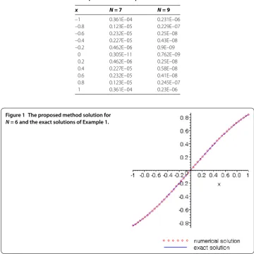
Example Consider the linear nonhomogeneous IVP [],
y(x) +xy(x) – y(x) =xcosx– sinx (.)
with the initial conditions
y() = and y() =
for which the exact solution isye(x) =sinx.
Table 1 Absolute errors of Example 1 at different points
x N= 7 N= 9
–1 0.361E–04 0.231E–06
–0.8 0.123E–05 0.229E–07
–0.6 0.232E–05 0.25E–08
–0.4 0.227E–05 0.43E–08
–0.2 0.462E–06 0.9E–09
0 0.305E–11 0.762E–09
0.2 0.462E–06 0.25E–08
0.4 0.227E–05 0.58E–08
0.6 0.232E–05 0.41E–08
0.8 0.123E–05 0.245E–07
1 0.361E–04 0.23E–06
Figure 1 The proposed method solution for
N= 6 and the exact solutions of Example 1.
Table 2 L∞Errors of Example 2 for differentNvalues
N Present method Haar wavelet based algorithm [37]
B-spline wavelet algorithm [38]
L∞ L∞ L∞
9 9.715E–05 -
-16 5.728E–07 2.9051E–04
-32 3.454E–08 7.4812E–05
-64 1.010E–08 1.8956E–05 2.5E–05
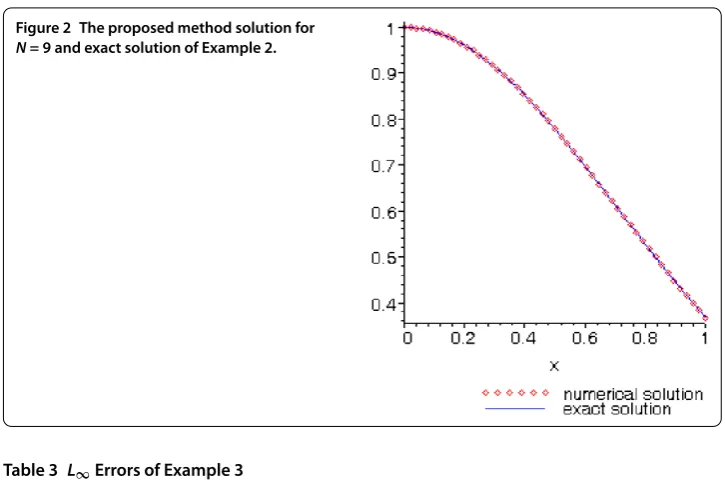
Example Consider now a linear homogeneous BVP
–y= – xy (.)
with Neumann boundary conditions
y() = and y() = –/e,
which is known to have the exact solutionye(x) =e–x.
repre-Figure 2 The proposed method solution for
N= 9 and exact solution of Example 2.
Table 3 L∞Errors of Example 3
N Present method B-spline wavelet algorithm [38]
L∞ L∞
8 2.58E–06
-16 8.94E–09
-32 4.04E–09 9.4E–05
64 2.09E–09 2.0E–05
sentation of the approximationyawith the exact solutionyeis also presented in Figure .
It is very promising to note that althoughL∞errors of the solutions to the problem (.) forN= in [, ] are given .E– and .E–, respectively, almost the same level of error has been achieved by the Fibonacci approach as .E– only forN= .
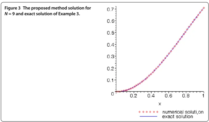
Example Consider a linear nonhomogeneous BVP
y(x) + y(x) = , x∈[, ] (.)
with boundary conditions
y() = , y() =sin(),
whose exact solution isye(x) =sin(x). A comparison ofL
∞errors of our approach and B-spline wavelet algorithm [] has been shown in Table for different values ofN. The exact and the approximate solutions of Example forN= are plotted in Figure .
5 Conclusion
Figure 3 The proposed method solution for
N= 9 and exact solution of Example 3.
Chebyshev polynomial method, the Fibonacci approach does not require interval trans-lation of the problem to an appropriate domain. Then, the reliability and efficiency of the method are verified by some illustrative examples of the boundary value problems. When the results are compared with some existing methods, the proposed method demonstrates its power in accuracy.
Competing interests
The authors declare that they have no competing interests.
Authors’ contributions
The authors have equal contributions to each part of this article. All the authors read and approved the final manuscript.
Author details
1Department of Mathematics, Faculty of Science, Selcuk University, Konya, Turkey.2Yayladagı Vocational School, Mustafa
Kemal University, Hatay, Turkey.
Acknowledgements
The authors would like to thank the editor and referees for their valuable comments and remarks, which led to a great improvement of the article. Also, authors would like to thank the Selcuk University and TUBITAK for their support. Authors reveal here that this study was partially presented orally at the International Congress in Honour of Professor Hari M Srivastava, August 23-26, 2012, Bursa, Turkey.
Received: 10 May 2013 Accepted: 6 August 2013 Published: 27 August 2013
References
1. Lebedev, NN: Special Functions and Their Applications. Prentice Hall, London (1965) (Revised Eng. ed.: translated and edited by Silverman, RA (1972))
2. Yudell, LL: The Special Functions and Their Approximations, vol. 2. Mathematics in Science and Engineering (Bellman, R (ed.)), vol. 53. Academic Press, New York (1969)
3. Wang, ZX, Guo, DR: Special Functions. World Scientific, Singapore (1989)
4. Sahin, A, Dag, I, Saka, B: A B-spline algorithm for the numerical solution of Fisher’s equation. Kybernetes37(2), 326-342 (2008)
5. Doha, EH, Bhrawy, AH, Saker, MA: On the derivatives of Bernstein polynomials: an application for the solution of high even-order differential equations. Bound. Value Probl.2011, 829543 (2011)
6. Celik, I, Gokmen, G: Approximate solution of periodic Sturm-Liouville problems with Chebyshev collocation method. Appl. Math. Comput.170(1), 285-295 (2005)
7. Sezer, M, Karamete, A, Gulsu, M: Taylor polynomial solutions of systems of linear differential equations with variable coefficients. Int. J. Comput. Math.82(6), 755-764 (2005)
8. Kadalbajoo, MK, Aggarwal, VK: Numerical solution of singular boundary value problems via Chebyshev polynomial and B-spline. Appl. Math. Comput.160, 851-863 (2005)
9. Lamnii, A, Mraoui, H, Sbibih, D, Tijini, A, Zidna, A: Spline collocation method for solving linear sixth-order boundary value problems. Int. J. Comput. Math.85(11), 1673-1684 (2008)
11. Fornberg, B: A Practical Guide to Pseudospectral Methods. Cambridge University Press, New York (1996) 12. Boyd, JP: Chebyshev and Fourier Spectral Methods, 2nd edn. Dover, New York (2000)
13. Canuto, C, Hussaini, MY, Quarteroni, A, Zang, TA: Spectral Methods: Fundamentals in Single Domains. Springer, Berlin (2006)
14. Agarwal, RP, O’Regan, D: Ordinary and Partial Differential Equations with Special Functions Fourier Series and Boundary Value Problems. Springer, New York (2009)
15. Sezer, M, Kaynak, M: Chebyshev polynomial solutions of linear differential equations. Int. J. Math. Educ. Sci. Technol.
27(4), 607-618 (1996)
16. Sezer, M, Do ˘gan, S: Chebyshev series solutions of Fredholm integral equations. Int. J. Math. Educ. Sci. Technol.27(5), 649-657 (1996)
17. Akyüz, A, Sezer, M: A Chebyshev collocation method for the solution of linear integro-differential equations. Int. J. Comput. Math.72, 491-507 (1999)
18. Sezer, M, Kesan, C: Polynomial solutions of certain differential equations. Int. J. Comput. Math.76(1), 93-104 (2000) 19. Mason, JC, Handscomb, DC: Chebyshev Polynomials. CRC Press, Boca Raton (2003)
20. Akyüz-Da¸scıo ˘glu, A: Chebyshev polynomial solutions of systems of linear integral equations. Appl. Math. Comput.
151, 221-232 (2004)
21. Celik, I: Solution of magnetohydrodynamic flow in a rectangular duct by Chebyshev collocation method. Int. J. Numer. Methods Fluids66(10), 1325-1340 (2011)
22. Gurefe, N, Kocer, EG, Gurefe, Y: Chebyshev-Tau method for the linear Klein-Gordon equation. Int. J. Phys. Sci.7(43), 5723-5728 (2012)
23. Bhrawy, AH, A-Shomrani, MM: A shifted Jacobi-Gauss-Lobatto collocation method for solving nonlinear fractional Langevin equation involving two fractional orders in different intervals. Bound. Value Probl.2012, 62 (2012) 24. Li, H, Ma, H: Shifted Chebyshev collocation domain truncation for solving problems on an infinite interval. J. Sci.
Comput.18(2), 191-213 (2003)
25. Parand, K, Dehghan, M, Pirkhedri, A: Sinc-collocation method for solving the Blasius equation. Phys. Lett. A373, 4060-4065 (2009)
26. Yalcinbas, S, Aynigul, M, Sezer, M: A collocation method using Hermite polynomials for approximate solution of pantograph equations. J. Franklin Inst.348, 1128-1139 (2011)
27. Kaya, B, Kurnaz, A, Koc, AB: Exponential Chebyshev Polynomials. Paper presented at the 3rd Conferences of the National Ere ˘gli Vocational High School, University of Selcuk, Ere ˘gli, 28-29 April (2011) (in Turkısh)
28. Boyd, JP: Rational Chebyshev spectral methods for unbounded solutions on an infinite interval using polynomial-growth special basis functions. Comput. Math. Appl.41, 1293-1315 (2001)
29. Guo, B, Shen, J, Wang, Z: Chebyshev rational spectral and pseudospectral methods on a semi-infinite interval. Int. J. Numer. Methods Eng.53, 65-84 (2002)
30. Sezer, M, Gülsu, M, Tanay, B: Rational Chebyshev collocation method for solving higher-order linear ordinary differential equations. Numer. Methods Partial Differ. Equ.27(5), 1130-1142 (2011)
31. Gulsu, M, Gurbuz, B, Ozturk, Y, Sezer, M: Laguerre polynomial approach for solving linear delay difference equations. Appl. Math. Comput.217, 6765-6776 (2011)
32. Byrd, PF: Expansion of analytic functions in polynomials associated with Fibonacci numbers. Fibonacci Q.1(1), 12-29 (1963)
33. Horadam, AF, Mahon, BJM: Pell and Pell-Lucas polynomials. Fibonacci Q.23(1), 7-20 (1985)
34. Falcon, S, Plaza, A: Thek-Fibonacci sequence and the Pascal 2-triangle. Chaos Solitons Fractals33(1), 38-49 (2007) 35. Falcon, S, Plaza, A: Onk-Fibonacci sequences and polynomials and their derivatives. Chaos Solitons Fractals39,
1005-1019 (2009)
36. Sezer, M, Gulsu, M: Solving high-order linear differential equations by a Legendre matrix method based on hybrid Legendre and Taylor polynomials. Numer. Methods Partial Differ. Equ.26(3), 647-661 (2010)
37. Siraj-ul-Islam, Aziz, I, Sarler, B: The numerical solution of second-order boundary-value problems by collocation method with the Haar wavelets. Math. Comput. Model.52, 1577-1590 (2010)
38. Lakestani, M, Dehghan, M: The solution of a second-order nonlinear differential equation with Neumann boundary conditions using semi-orthogonal B-spline wavelets. Int. J. Comput. Math.83(8-9), 685-694 (2006)
doi:10.1186/1687-1847-2013-262