Using global magnetospheric models for simulation and interpretation of
Swarm
external field measurements
T. Moretto1∗, S. Vennerstrøm2, N. Olsen2, L. Rast¨atter1, and J. Raeder3 1NASA Goddard Space Flight Center, Greenbelt, Maryland, U.S.A.
2Danish National Space Center, Copenhagen, Denmark
3Space Science Center, University of New Hampshire, Durham, New Hampshire, U.S.A.
(Received January 5, 2004; Revised September 19, 2005; Accepted September 29, 2005; Online published April 14, 2006)
We have used a global model of the solar wind magnetosphere interaction to model the high latitude part of the external contributions to the geomagnetic field near the Earth. The model also provides corresponding values for the electric field. Geomagnetic quiet conditions were modeled to provide simulated external contributions relevant for internal field modeling. These have proven very valuable for the design and planning of the up-coming multi-satelliteSwarmmission. In addition, a real event simulation was carried out for a moderately active time interval when observations from the Ørsted and CHAMP sattelites were available. Comparisons between the simulation results and the satellite observations for this event demonstrate the current level of validity of the global model. We find that the model reproduces quite well the region 1 current system and nightside region 2 currents whereas it consistently underestimates the dayside region 2 currents and overestimates the horizontal ionospheric closure currents in the dayside polar cap. Furthermore, with this example we illustrate the great benefit of utilizing the global model for the interpretation ofSwarmexternal field observations and, likewise, the potential of usingSwarmmeasuremnets to test and improve the global model.
Key words: Ionospheric currents, field-aligned currents, global magnetospheric simulation, low-altitude satel-lites.
1.
Introduction
The geomagnetic activity that is measured in the near-Earth space environment is the combined effect of vast, complex, and continually changing electric current systems in the Earths magnetosphere and ionosphere. Accurate pa-rameterization of these current systems as well as improved understanding of the physical processes that drive them constitute an important goal of the planned multi-satellite
Swarmmission (Friis-Christensenet al., 2006). This is nec-essary for advancing the inclusion of the external fields in the internal field modeling and for improving the data selec-tion and correcselec-tion for this modeling. In addiselec-tion, the exter-nal current systems are a key ingredient in the solar wind-magnetosphere-ionosphere system the full understanding of which is currently one of the main objectives within the field of space plasma physics.
The wide-spread and dynamic nature of the external cur-rent systems means that it is necessary to invoke models when interpreting sparsely distributed observations such as measurements from a few near-Earth spacecraft as sug-gested for the Swarmmission. Previously, empirical sta-tistical models were mainly used for this purpose. Promi-nent examples are the model of high-latitude ionospheric
∗Now at Division of Atmospheric Sciences, National Science
Founda-tion, Arlington, Virginia, U.S.A.
Copyright cThe Society of Geomagnetism and Earth, Planetary and Space Sci-ences (SGEPSS); The Seismological Society of Japan; The Volcanological Society of Japan; The Geodetic Society of Japan; The Japanese Society for Planetary Sci-ences; TERRAPUB.
current distributions developed by Friis-Christensenet al.
(1985); the model of high-latitude ionospheric electrical potential distributions developed by Weimer (1995, 2001), and the recent model of high latitude field-aligned cur-rents derived from geomagnetic satellite observations by Papitashvili et al. (2002). Similarly, empirical models that describe the magnetic variation at non-polar latitudes, such as the quiet day Sq current system and the equa-torial electrojet, exist (e.g., Sabaka et al., 2002). Self-consistent, physics-based models for the various parts of the complex solar wind- magnetosphere-ionosphere system are currently fast emerging. Global Magneto-Hydro-Dynamic (MHD) simulations are first-principle physics models that provide a self-consistent description of the large-scale mag-netospheric configuration and dynamics as well as basic magnetosphere-ionosphere coupling driven by input solar wind parameters. A number of such models exist at present (e.g. Raeder, 2003). For the high-latitude ionospheres they provide realistic, and self-consistent, distributions of the horizontal electric field and currents in the ionosphere as well as the field aligned currents that couple the high lati-tude ionosphere to the outer magnetosphere. The validation of the global simulation models by comparison with obser-vations is a very important task that currently attracts a lot of attention (e.g. Raederet al., 1997; Kelleret al., 2002; Ohtani and Raeder, 2004; Korthet al., 2004 and many oth-ers).
This paper together with the two accompanying papers by Vennerstrømet al.(2006) and Ritter and L¨uhr (2006),
present the first results of utilizing a global MHD model for the interpretation and simulation of Swarm external field measurements. Three different simulations represent-ing quiet and moderately disturbed geomagnetic conditions have been performed. Focus here is on the effect of the high latitude ionospheric currents and corresponding near-Earth field aligned currents from a real event simulation of a time interval with moderate geomagnetic activity. We show ex-amples of comparisons between the simulation results and measurements from the Ørsted and CHAMP geomagnetic satellite missions for this event. These serve to demonstrate the current level of validity of the global model for simu-latingSwarmobservations and to illustrate the potential for very fruitful collaborations between global MHD model de-velopers and theSwarmmission.
The global simulation model is described in the following section. Then follows a description of how the resulting magnetic and electric fields were calculated on a global grid at satellite altitudes. Next, follows a presentation of the three simulations that were performed for theSwarmstudies so far. The next section presents the comparison between the results for the real event simulation and observations from the Ørsted and CHAMP satellites. The final section gives a summary and discusses future plans.
2.
The Open Geospace General Circulation
Model
Realistic estimates of the currents in the ionosphere and magnetosphere responsible for the external magnetic field contributions at polar latitudes are provided for this study by the Open Geospace General Circulation Model (Open-GGCM) (e.g. Raeder et al., 1995; Raeder et al., 1998) that is run at the Community Coordinated Modeling Cen-ter (CCMC) at NASA Goddard Space Flight CenCen-ter. The model solves the resistive MHD equations in the magneto-sphere. The simulation was run on a grid 160×60×60 in size, spanning from−255 Earth radii (RE) to 33 RE in
the GSE X direction and from−48 RE to 48 RE in the
GSE Y and Z directions. The grid has finest resolution of 0.4 RE close to the inner magnetospheric boundary. The
model also includes a magnetosphere-ionosphere coupling module that not only maps the field-aligned current den-sities, J, into the ionosphere and the potential back into the magnetosphere, but also computes electron precipitation parameters and the ionospheric Hall and Pedersen conduc-tances using empirical relations in a self-consistent manner (Raederet al., 1998). Field-aligned currents are calculated close to the inner boundary of the magnetospheric part of the simulation (at 4RE) and are used as input to solve the
ionospheric potential equation. The field-aligned currents are mapped from points in the magnetosphere(rM, ϑM, λ)
The polar ionosphere is treated as a two-dimensional spher-ical shell, thus the ionospheric potential equation reads (e.g. Kelley, 1989; Raeder, 2003):
∇ ·· ∇= −JsinI (2)
with the boundary condition for the electric potential:= 0 at the magnetic equator.is the ionospheric conductance (i.e., height integrated conductivity) tensor, given by:
=
where H is the Hall conductance, P is the Pedersen
conductance, ϑ is magnetic co-latitude,λis the magnetic longitude andI is the magnetic field inclination angle.
The ionospheric Hall and Pedersen conductances play a key role in determining the ionospheric electrodynam-ics of the model. In the implementation of the model used for this study, they are computed from empirical formulas. The conductances are proportional to the ionospheric elec-tron density (mostly dominated by the E-region), which is mainly determined by solar EUV irradiance and precipita-tion of magnetospheric electrons. The contribuprecipita-tion to the conductance from the former is reliably parameterized by the solar radio flux parameter,F10.7, together with the solar
zenith angle (Moen and Brekke, 1993). The contributions to the conductance from magnetospheric electron precipi-tation are parameterized by the energy flux and mean en-ergy of the precipitating electrons (Robinsonet al., 1987). For the diffuse precipitation (from pitch angle scattering of hot magnetospheric electrons) these are parameterized, in turn, by the magnetospheric electron temperature and den-sity, which are approximated by the density and tempera-ture values from the magnetospheric part of the simulation. Additional discrete electron precipitation (auroral electrons accelerated by field-aligned potential drops) is parameter-ized by the field-aligned current density through the Knight relation (Knight, 1972).
The open-GGCM is driven by solar wind plasma and magnetic field conditions specified at the upstream simu-lation box boundary at 33 RE. For the simulation of real
events, the solar wind observations must be propagated from a solar wind monitor satellite to this input position. The Earth magnetic field is approximated by a dipole with fixed orientation during the entire simulation run. Standard outputs from the model simulation include the magneto-spheric plasma parameters (density, plasma pressure, veloc-ity, magnetic field, and current densities), the ionospheric parameters (electric potential, field-aligned currents, and Hall and Pedersen conductances), and the mean energy and energy flux for the electron precipitation.
the physical assumptions and approximations in the model (Raeder, 2003). It is outside the scope of this paper to do full justice to the many past and ongoing efforts on this prob-lem. For the ionospheric parameters that are the focus of this study, obvious objects for validation are the inherent limitations in the model provided by the electrostatic, thin-sheet approximation of the ionosphere and the reliance on empirical formulae for the calculating the conductance. Re-cent efforts have focused on replacing the simple sheet ap-proximation for the ionosphere with fully dynamical multi-fluid ionosphere-thermosphere models (e.g. Raeder et al., 2001; Ridley et al., 2003). Specifically, this eliminates the need for invoking the Robinson formula in calculat-ing the conductance contribution from electron precipita-tion and includes the ionospheric dynamo (neutral winds) effect. Raederet al.(2001) found that this can significantly change the conductance and improve the comparison with ground based observations of the auroral electrojets. Rid-leyet al.(2003) reported neutral wind effects on the field-aligned currents in the ionosphere of the order of 10–20 percent, with the strongest effect observed immediately fol-lowing a northward turning of the IMF. Efforts to go be-yond the electrostatic magnetosphere-ionosphere coupling adopted in the current models (e.g. allowing for parallel electric fields) are also under way (Lotko, 2004). Valida-tion and improvement projects like these remain an impor-tant ongoing effort within the global modeling community at present. Since implementing models to run at the CCMC, this is increasingly becoming a wider community effort as well, and the study presented here is a contribution to this larger effort.
3.
Simulated
Swarm
external magnetic and
elec-tric field contributions
To produce estimates of the Swarmexternal fields the standard outputs from the open-GGCM model must be aug-mented. First, the three-dimensional distribution of the field-aligned currents in the “gap” between the inner bound-ary of the magnetospheric part of the simulation (at 4 RE)
and the ionosphere (at 90 km altitude) were calculated by mapping of the field-aligned current density as described by Eq. (1). This was done on a spherical grid that is equidis-tant in the angular coordinates(ϑ, λ)with 129 and 128 grid points, respectively, and has a distribution in the radial co-ordinate given by:
in the radial direction. The horizontal ionospheric (sheath) current distribution is calculated (on the corresponding grid in ϑ and λ ) from the ionospheric electric potential and conductances by:
whereEhoriz is the ionospheric electric field. Finally, the
magnetospheric current distribution was calculated on the continuation of the spherical grid with equidistant spac-ing of 0.5 RE in the radial component from 4.5 RE out
to 20 RE (32 grid points). All together, these
contribu-tions provide the global three-dimensional current distribu-tion from which the magnetic field measurements atSwarm
altitudes were calculated.
For any given distribution of current density,J, the cor-responding magnetic field can be calculated directly by in-tegration according to Biot–Savart’s law (see Vennerstrøm
et al., 2006) The main problem with this approach is that the computation becomes very time-consuming when the number of grid-points is large. The advantage of this direct approach, on the other hand, is that it allows for the com-parison between the contributions from different parts of the total current distributions. Results from such an analysis are presented by Vennerstrømet al.(2006).
A computationally very efficient technique for calculat-ing the magnetic field due to a given current distribution was developed by Engels and Olsen (1998). The method is based on the decomposition of divergence free vector fields into poloidal and toroidal parts following Stern (1976) and Backus (1986). Assuming that the time and length scales of the current density and magnetic fields considered are such that displacement currents can be neglected, which is equivalent to a non-divergent current density divJ=0, and using that divB = 0 everywhere, it is possible to decom-pose both the current densityJand the associated magnetic fieldBinto poloidal and toroidal parts, both of which can be expressed by scalar fields. The toroidal part of the magnetic field is determined by the poloidal part of the current density and the poloidal part of the magnetic field is determined by the toroidal part of the current density, independently and by fairly simple relations.
In the implementation of the technique adopted for this work, spherical harmonic expansions of the toroidal and poloidal scalar functions of the current density (and hence of those of the magnetic field) of degree and order 60 have been used. The magnetic field vector components corre-sponding to each of the current density distributions pro-duced by the global model have been calculated on a spher-ical grid identspher-ical to the one used for the current densities. This product provided the basis for the analysis presented in the accompanying paper by Ritter and L¨uhr (2006)
ACE March 9, 2002
-5 0 5 10
GSM
B
[nT]
14 18 UT
300 400 500
V
[km/s]
2 4 6 8
n
[cm
-3 ]
12 16
Bx
By
Bz
n
v
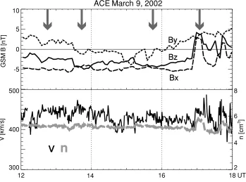
Fig. 1. Displayed are ACE observations of the interplanetary magnetic field and solar wind speed and number density that was used to drive the global magnetosphere model for March 9, 2002 12–18 UT. A delay of 55 min has been added to the spacecraft measurements to account for the solar wind propagation.
4.
Swarm
Study Simulations
While geomagnetic activity is driven by the combination of a wide variety of conditions in the solar wind and mag-netosphere, including their time-history, the single most de-cisive parameter is the north-south component (BZ) of the
interplanetary magnetic field (IMF). Keeping all other pa-rameters at average values, a small, positive (northward) IMFBZ component generally will produce very low levels
of geomagnetic activity. A small negative IMF BZ
com-ponent, in contrast, is generally associated with moderate geomagnetic activity. Following the objective of theSwarm
mission, simulations were first made for geomagnetic quiet and moderately disturbed conditions.
One simulation was driven by average density and solar wind values with the IMFBZ component changing slowly
from a small positive to a small negative value over 8 hours. Specifically, the solar wind conditions used as input for the first simulation were: constant density, velocity, and tem-perature of 7 cm−3, 400 km/s (along the Sun-Earth axis),
and 1.4×10⁵ K, respectively; IMF with zero B
Y and BX
GSM components andBZ component that changes linearly
from +5.5 nT to −5.5 nT over the 8 hours of the simu-lation. A standard value of 150×10−22W/m2/Hz, was
used for the F10.7 parameter. Dipole tilt was zero making
the model output exactly symmetric between the Northern and Southern hemispheres. The results from this simula-tion have been used in the analyses presented in the two ac-companying papers of Vennerstrømet al.(2006) and Ritter and L¨uhr (2006). Another simulation was performed with the same solar wind driving conditions but applying a tilt of the dipole axis. This allows for comparative analyses of the results for winter and summer conditions at the two po-lar regions. A dipole tilt of−25 degrees in the X-Z plane
was included, simulating winter conditions for the Northern hemisphere and summer conditions for the Southern hemi-sphere.
Finally, a simulation driven by actual solar wind observa-tions for a quiet to moderately active period was performed to allow for the comparison of the model results with mag-netic field measurements from the Ørsted and CHAMP satellites. The time interval of March 9, 2002, 06–18 UT was chosen for the simulation. The simulations were per-formed as so-called runs on request and the modeling re-sults from all of the runs are available at the CCMC web-site (http://ccmc.gsfc.nasa.gov), keyword: swarm. Output from the simulations have been saved every 10 minutes.
For the real event simulation, solar wind observations from the ACE spacecraft were propagated to the simulation inflow boundary at 33REupstream of the Earth. Focus here
is on the more active, second half of the real event interval (12–18 UT) and the solar wind parameters that were used as input for this part of the real event simulation are shown in Fig. 1. They exhibit fairly stable values for the number density and velocity of approximately 5 cm−3and 430 km/s,
respectively. Until the abrupt change just before 17 UT, the IMFBZ component is southward with values between
−2 nT and −5 nT. The IMF BY component starts out
with a small positive value, then changes to near zero and slightly negative, and finally ends up again with a significant positive value. We note that the IMFBX component has a
value of−5 nT throughout most of the interval but that this was not included in the simulation. A dipole tilt appropriate for the date and time was applied and was updated every two hours of the run.
50o
Mag.Lat.
North
18
06
00 MLT
0.3 A/m
1300 UT
-50o
Mag.Lat.
South
18
06
00 MLT
50o
Mag.Lat.
North
18
06
00 MLT
0.3 A/m
1400 UT
-50o
Mag.Lat.
South
18
06
00 MLT
50o
Mag.Lat.
North
18
06
00 MLT
0.3 A/m
1600 UT
-50o
Mag.Lat.
South
18
06
00 MLT
50o
Mag.Lat.
North
18
06
00 MLT
0.3 A/m
1720 UT
-50o
Mag.Lat.
South
18
06
00 MLT
0.0
1.5 Am
μ
-2-1.5
J
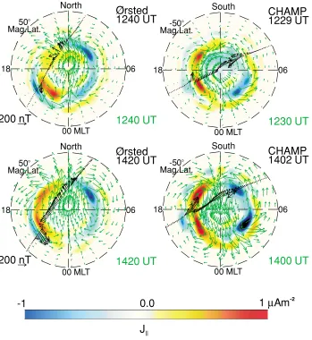
||and field aligned currents, with only very small contribu-tions from the distant magnetopause and tail currents (Ven-nerstrømet al., 2006 (this issue)). Figure 2 displays polar maps of the distribution of these current sources over the high latitude ionosphere in both hemispheres at four dif-ferent times during the simulation. The selected times are marked by the broad arrows in Fig. 1, including an addi-tional 15 min delay to account for the time it takes for the solar wind to propagate through the magnetosheath and for any changes to the dayside currents to get established (e.g. Ruohoniemiet al., 2002).
The first pattern at 1300 UT shows well-defined region 1 currents, out of the ionosphere (yellow) on the dusk side and into the ionosphere (blue) on the morning side, roughly along the 75◦latitude circle. This is consistent with the IMF having a small negative BZ-component at this time (Iijima
and Potemra, 1976). An additional set of field aligned rents in the dayside polar caps (poleward of the region 1 cur-rents) with opposite polarity in the two hemispheres (yel-low in the northern and blue in the southern) are also ob-served. This is consistent with the significant positive BY
-component that is present in the IMF at this time (Friis-Christensenet al., 1985). This gives rise to a distinct asym-metry also for the horizontal currents on the dayside be-tween the northern and southern hemisphere. At the time of the next set of plots at 1400 UT, the IMFBY-component
is close to zero and, correspondingly, the polar cap currents are no longer present. As expected for this case, the cur-rent patterns for the two hemispheres are now very simi-lar. They also have intensified slightly as a result of the increased southward IMF. At the time of the next set of maps at 1600 UT, the northern hemisphere map indicates fairly steady conditions for the dayside. Variations caused by dynamic changes in the tail magnetosphere (substorms) are seen in the nightside currents. The pattern for the south-ern hemisphere at this time is similar but the ionospheric current intensities in the polar cap region are lower. This is a result of reduced conductance in the southern dayside ionosphere as compared to the northern caused by the UT-dependence of the dipole tilt. The dipole tilt is at its maxi-mum (7◦in the X-Z plane) around this time with the North-ern magnetic pole pointing in the direction towards the sun. The last set of patterns at 1720 UT show much reduced rent intensities both for the field aligned and horizontal cur-rents reflecting the northward IMF conditions at this time. Also consistent with the northward IMF is the presence of a pair of currents of opposite polarity in the dayside of each polar cap. These are the so-called NBZ currents and the asymmetry displayed between the two currents of the pairs in both hemispheres as well as between the hemispheres is consistent with the influence of the significant positiveBY
-component in the IMF at this time (e.g. Vennerstrømet al., 2002; Vennerstrømet al., 2005).
5.
Comparison with Ørsted and
CHAMPMag-netic Field Observations
On the date of the real event simulation (March 9, 2002), the orbit planes for the Ørsted (Neubertet al., 2001) and CHAMP (Reigber et al., 2002) satellites are fairly close. Between 12 UT and 14 UT, the satellites are moving nearly
oppositely in their orbits so that they cross opposite poles almost simultaneously. We use the polar passes from two consecutive orbits during this period as our first illustration of the comparison between the simulation results and the magnetic field observations.
Figure 3 shows polar maps of the horizontal magnetic variation vectors (green arrows) together with the field-aligned current distribution (background color scale) from the simulation for the two crossings over the northern po-lar region by Ørsted (left panels) and the corresponding south polar crossings by the CHAMP satellite (right pan-els). Matching the difference in the orbits, altitudes of 700 km and 450 km have been used for the maps for the Ørsted and CHAMP crossings, respectively. The observa-tions are overlaid and are displayed as black arrows along the satellite tracks. The shown vectors are 5 sec averages derived from 1 sec vector magnetic field variation data from the satellites. The duration of the polar crossings is approx-imately 20 minutes and the time quoted for each map is the time when the satellite passes closest to the magnetic pole. The time in green at the bottom right of each panel is the time of the model output (green vectors and background color image).
Overall, the comparison in Fig. 3 shows remarkably good agreement between the model results and the satellite ob-servations. In particular, the model seems to predict the strength and location of the region 1 currents (and their re-lated magnetic variations) quite well. The main problem, on the other hand, seems to be the dayside polar cap area. This is especially clear for the CHAMP southern cross-ing at 1400 UT (lower right panel in Fig. 3). In this case, the model predicts rather strong and fairly uniform mag-netic field vectors across the polar cap that do not match the CHAMP observations very well. The model magnetic field vectors reflect the presence in the model ionospheric current system at this time of strong horizontal currents over the dayside polar cap area as seen in Fig. 2 (second row). Our comparison therefore would indicate that these are not com-pletely realistic. We speculate that this could result from the region 2 currents not being reproduced well enough in the simulation which then enforces too much closure of the re-gion 1 currents across the polar cap. Some further evidence in support of this view is presented below. The magnetic effect of the horizontal currents decrease rapidly with alti-tude (Vennerstrømet al., 2006) which is why the problem is more pronounced for CHAMP than for Ørsted.
0.0
1 Am
μ
-2-1
J
|| North50o
Mag.Lat.
18 06
00 MLT
Ørsted
1240 UT
200 nT
1240 UT
South
-50o
Mag.Lat.
18 06
00 MLT
CHAMP
1229 UT
1230 UT
South
-50o
Mag.Lat.
18 06
00 MLT
CHAMP
1402 UT
1400 UT
North50o
Mag.Lat.
18 06
00 MLT
Ørsted
1420 UT
200 nT
1420 UT
Fig. 3. Polar maps of the horizontal magnetic variation vectors derived from the open-GGCM simulation of March 9, 2002 12–18 UT and measured by Ørsted or CHAMP are shown for four selected polar crossings. The background color scale shows the field aligned current density distributions like in Fig. 2. The horizontal magnetic variations from the model are shown as green arrows and the satellite observations as black arrows.
ORSTED15998 North
12:29 12:51 UT
-600 -400 -200 0 200 400 600
dB
[nT]
MODEL 1230 UT
BHORBR
ORSTED15998 North
200 nT
ORSTED15999 North
14:09 14:32 UT
-600 -400 -200 0 200 400 600
dB
[nT]
MODEL 1410 UT
BHORBR
ORSTED15999 North
200 nT
CHAMP09294 South
12:19 12:39 UT
-600 -400 -200 0 200 400 600
dB
[nT]
MODEL 1230 UT
BHORBR
CHAMP09294 South
200 nT
CHAMP09295 South
13:52 14:13 UT
-600 -400 -200 0 200 400 600
dB
[nT]
MODEL 1400 UT
BHORBR
CHAMP09295 ]
200 nT
ORSTED15998 North
12:29 12:51 UT -2
-1 0 1 2
J||
[
μ
Am
-2 ]
1230 UT
ORSTED15999 North
14:09 14:32 UT -2
-1 0 1 2
J||
[
μ
Am
-2 ]
1410 UT
CHAMP09294 South
12:19 12:39 UT -2
-1 0 1 2
J||
[
μ
Am
-2 ]
1230 UT
CHAMP09295 South
13:52 14:13 UT -2
-1 0 1 2
J||
[
μ
Am
-2 ]
1410 UT
R0
R2 R1
R1 R2
R1
R0
R1 R2
R1
R1 R2 R0
R1
R2
R1 R2
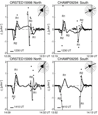
Fig. 5. Along track comparisons between model predictions and measurement based estimates of the field-aligned current density for the four polar crossings of Fig. 3. Model results are thick curves. Crosses represent 15 sec averages of the current density estimates and the thin lines show 45 sec averages. Negative values are for currents flowing into the ionosphere and positive values for currents flowing out.
much smaller magnitude than the horizontal perturbations (Vennerstrømet al., 2006), their almost sole source being the horizontal ionospheric currents. This also means that we should not be surprised to find that they exhibit the same problem that we pointed out for the horizontal perturbations of sometimes overestimating the effect in the polar cap. The second southern CHAMP crossing (lower right panel in Figs. 3 and 4) is a prominent example of this.
For the horizontal variations, the single track compar-isons largely confirm the findings that the polar maps in Fig. 3 convey. However, they also illustrate an inherent but important problem with using single space craft observa-tions (or other sparse measurement sources) for testing of the model results. Namely, that even small displacements of structures, whose size; shape; and amplitude might oth-erwise be reproduced quite well by the model, show up as large discrepancies that may be misleading. This point is illustrated well by the nightside parts of the two Ørsted crossings (panels on the left in Figs. 3 and 4). The predicted nightside perturbations for the first crossing are much larger than observed (left part of upper left panel in Fig. 4), but from the total polar pattern in Fig. 3 (upper left panel) it is clear that the field-aligned current structure need only be rotated eastward by approximately 15◦ to give a much
im-proved match. In contrast, the nightside part of the follow-ing northward Ørsted crossfollow-ing show a near perfect match (lower left panels in Figs. 3 and 4) between the predicted and observed perturbations. The field-aligned current struc-tures in this case are much more sheet-like (wide-spread and near-homogeneous in longitude) and therefore are much less sensitive to the exact location of the structures in this direction relative to the satellite track. Part of this problem, of course, may be caused by inaccuracies in the mapping in-volved when deriving the satellite track, which is geograph-ically defined, and the model which is defined in terms of a magnetic dipole system.
A complimentary view of the comparison is offered by the field-aligned currents. Adopting the infinite (east-west aligned) current sheet approximation for the field-aligned currents, a commonly used estimate for the field-aligned current density along the satellite track based on the mag-netic field measurements (Ritter and L¨uhr, 2006) is given by:
j= μ d B⊥E
0·dt·v⊥·cosα
(5)
whered B⊥Eis the difference between single measurements
0.0
1 Am
μ
-2-1
J
|| North50o
Mag.Lat.
18 06
00 MLT
Ørsted
1740 UT
200 nT
1740 UT
North
50o
Mag.Lat.
18 06
00 MLT
CHAMP
1757 UT
1800 UT
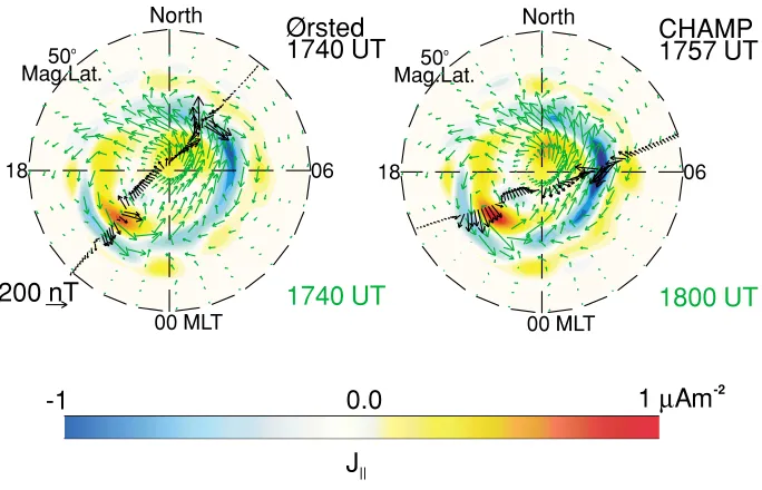
Fig. 6. Polar maps of the horizontal magnetic variation vectors derived from the open-GGCM simulation of March 9, 2002 12–18 UT and measured by Ørsted or CHAMP are shown for a two near-simultaneous North polar crossings. The background color scale shows the field aligned current density distributions like in Fig. 2. The horizontal magnetic variations from the model are shown as green arrows and the satellite observations as black arrows.
ORSTED16001 North
17:28 17:51 UT
-600 -400 -200 0 200 400 600
dB
[nT]
MODEL 1750 UT
BHORBR
ORSTED16001 North
200 nT
CHAMP09298 North
17:47 18:07 UT
-600 -400 -200 0 200 400 600
dB
[nT]
MODEL 1750 UT
BHORBR
CHAMP09298 North
200 nT
Fig. 7. Along track comparisons between model predictions and satellite observations of the horizontal and radial magnetic perturbations for the two polar crossings of Fig. 3. Model results are green arrows (horizontal magnetic vectors) and curves (magnitude of variation): dashed lines for the radial component and full lines for the horizontal component. Black and red dots in the upper tracks represent 5 sec averages of the magnitude of the horizontal and radial perturbations, respectively, measured by the satellites. Black arrows in the lower tracks display the measured horizontal magnetic variation vectors.
magnetic east direction (determined by the standard IGRF model); dt is the time difference between measurements, here 1 sec;v⊥is the projection of the satellite velocity into the plane perpendicular to the background magnetic field; andαis the angle of attack between the satellite track and the normal to the current sheet (assumed to be aligned in the local magnetic east-west direction). Figure 5 displays estimated current densities for the four polar crossings of Figs. 3 and 4 together with the corresponding field aligned current densities predicted by the global simulation. The latter are represented by thick black curves in the figure. The crosses represent 15 sec averages of the calculated 1 sec current density estimates and the thin lines represent 45 sec running averages of the same. This corresponds to spatial resolutions of approximately 100 km and 300 km, respec-tively. Estimates are only calculated for the parts of the satellite tracks that fulfill: α < 60◦. Where they could be identified with reasonable certainty, the main large-scale field-aligned current regions, Region 1, Region 2, and Re-gion 0 (or Cusp and Polar Cap currents) have been called out in the panels as R1, R2, and R0, respectively. These
R0
R2 R1
R1
R2
R1
R1
R2 R0 R2
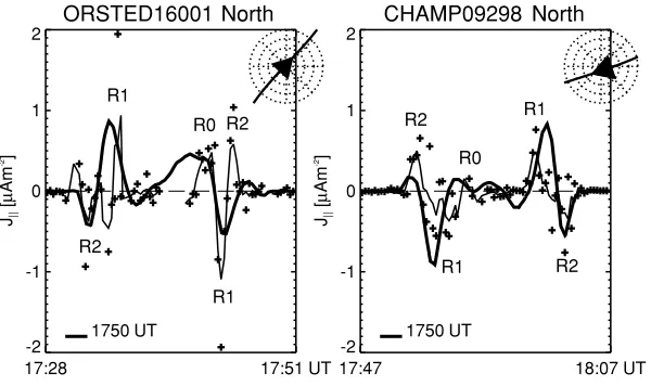
ORSTED16001 North
17:28 17:51 UT
-2 -1 0 1 2
J||
[μ
Am
-2 ]
1750 UT
CHAMP09298 North
17:47 18:07 UT
-2 -1 0 1 2
J||
[μ
Am
-2]
1750 UT
Fig. 8. Along track comparisons between model predictions and measurement based estimates of the field-aligned current density for the four polar crossings of Fig. 3. Model results are thick curves. Crosses represent 15 sec averages of the current density estimates and the thin lines show 45 sec averages. Negative values are for currents flowing into the ionosphere and positive values for currents flowing out.
same. In contrast, the region 2 currents seem to be consis-tently underestimated by the model. This tendency seems to get more pronounced as activity increases (from top row to bottom row of panels in the figure). These results sup-port the conjecture made earlier that the problem with the simulation overestimating the dayside polar cap magnetic measurements during active conditions is mainly a result of lacking realistic region 2 currents in the model.
As a second example of the comparison between the global model results and measurements from Ørsted and CHAMP, we present the results for a pair of near-simultaneous North-polar crossings close to the end of the simulation interval. In the same formats as earlier, Fig. 6 displays the polar maps, Fig. 7 the along-track perturba-tions, and Fig. 8 the field-aligned current densities. Note that now Ørsted crosses from the nightside to the dayside while CHAMP crosses in the opposite direction (from the dayside to the nightside). For this case, good agreement is found with the CHAMP observations on the nightside part of the crossing (right part of panel on the right) while the Ørsted observations (left part of panel on the left) in-dicate a more structured and complex current system than predicted. We believe that this is caused by Ørsted be-ing very close to the Harang-discontinuity, the position of which the model may not have predicted accurately. For the dayside parts (right part of left hand panel and left part of right hand panel), both satellite measurements are repro-duced quite well, though the region 2 current densities seem to be consistently underestimated as discussed for the first example.
6.
Summary and Outlook
We have described a set of tools that we have devel-oped to provide predictions for theswarmelectric and ex-ternal magnetic field measurements from global magneto-hydrodynamic simulations of the solar wind interaction with the Earth’s magnetosphere. Self-consistent sets of magnetospheric and ionospheric electric currents and corre-sponding electric and magnetic field perturbations atSwarm
altitudes have been produced for several different
geomag-netic activity conditions. These data sets were used in the analyses presented in the papers by Ritter and L¨uhr (2006) and Vennerstrømet al.(2006).
For validation of our approach and to illustrate the poten-tial of using the global MHD models for interpretation of theSwarmdata, a simulation of a real time interval was per-formed using solar wind measurements to drive the model. These results were compared with magnetic field perturba-tion measurements from the Ørsted and CHAMP satellites for a number of polar crossings during the simulation in-terval. The comparison showed good agreement on many general, large-scale features between the model results and the satellite observations. In particular, the model seems to predict the strength and pattern of the region 1 currents (and their related magnetic variations) quite well. The most important discrepancies were found in the dayside polar cap region during more geomagnetically active conditions in which the model predictions greatly overestimated the measured magnetic perturbations, particularly for the lower altitude spacecraft (CHAMP). The large amplitude mag-netic field perturbations in the model are caused by strong horizontal ionospheric currents flowing across the dayside polar cap providing closure for the dayside region 1 currents in the model. Hence, the problem is closely related to the weakness in the global MHD models of providing realistic region 2 currents. Our comparisons with the satellite obser-vations show clear examples of the region 2 currents on the dayside being underestimated by the model.
The present study clearly verifies the value and mutual benefit of close collaboration between the global magneto-spheric model developers and theSwarmmission. We have illustrated the unique capability of the global MHD mod-els to provide global context for theSwarmmeasurements and to allow physics based interpretations of the observa-tions. In turn, we have also demonstrated the unique ca-pability of theSwarmmission to provide accurate tests of important model variables and, through that, valuable feed-back to the model developers regarding the consistency and accuracy of the models. The development of realistic and precise predictive models is the main goal of current space weather research activities. Model validation through com-parisons with observations is a very important component hereof. Another important objective is the development of methods to further constrain the models by assimilation of observational data. It is obvious thatSwarmcan make valu-able contributions to both of these tasks. Immediately, in an obvious continuation of the efforts presented here and using observations from the current Ørsted and CHAMP missions as well as simulated futureSwarmdata a number of important questions can be addressed:
• What are the most important factors determining how well the model output match the measurements of magnetic fields and currents?
• How do we best define quantitative measures for the agreement to monitor improvements?
• How can theSwarmmeasurements be used in a sys-tematic way to drive space weather prediction models?
• How can theSwarmobservations best be used to fur-ther model development?
Acknowledgments. We gratefully acknowledge the use of the CHAMP vector magnetic field data courtesy of H. L¨uhr, GFZ Potsdam. The Ørsted Project was made possible by extensive support from the Ministry of Trade and Industry, the Ministry of Research and Information Technology, and the Ministry of Transport in Denmark. We thank the ACE SWEPAM and MAG instrument teams and the ACE Science Center for providing the ACE data. ESA (ESTEC) supported this study through contract No. 3-10901/03/NL/CB.
References
Backus, G., Poloidal and toroidal fields in geomagnetic field modeling,
Rev. Geophys.,24, 75, 1986.
De Zeeuw, D. L., S. Sazykin, R. A. Wolf, T. I. Gombosi, A. J. Rid-ley, and G. Toth, Coupling of global MHD code and an inner mag-netospheric model: Initial results, J. Geophys. Res., 109, A12219, doi:10.1029/2003JA010366, 2004.
Engels, U. and N. Olsen, Computation of magnetic fields within source regions of ionospheric and magnetospheric currents,J. Atm. Sol.-Terr. Physics,60, 1585, 1998.
Friis-Christensen, E., H. L¨uhr, and G. Hulot,Swarm: A constellation to study the Earth’s magnetic field,Earth Planets Space,58, this issue, 351–358, 2006.
Friis-Christensen, E., Y. Kamide, A. D. Richmond, and S. Matshusita, Interplanetary magnetic field control of high-latitude electric fields and currents determined from Greenland magnetometer data,J. Geophys. Res.,90, 1325, 1985.
Iijima, T. and T. A. Potemra, The amplitude distribution of field-aligned currents at northern high latitudes observed by Triad,J. Geophys. Res., 81, 2165, 1976.
Keller, K. A., M. Hesse, M. Kuznetsova, L. Rast¨atter, T. Moretto, T. I. Gombosi, and D. L. DeZeeuw, Global MHD modeling of the impact of a solar wind pressure change,J. Geophys. Res.,107, 1126, 2002. Kelley, M. C.,The Earth’s Ionosphere, Academic Press, New York, 1989.
Knight, S., Parallel electric fields,Planet. Space Sci.,21, 741, 1972. Korth, H., B. J. Anderson, M. J. Wiltberger, J. G. Lyon, and P. C.
An-derson, Intercomparison of ionospheric electrodynamics from the Irid-ium constellation with global MHD simulationsJ. Geophys. Res.,109, doi:10.1029/2004JA010428, 2004.
Lotko, W., Inductive magnetosphere-ionosphere coupling,J. Atm. Sol.-Terr. Physics,66, 1443, 2004.
Moen, J. and A. Brekke, The solar flux influence on quiet time conduc-tances in the auroral ionosphere,Geophys. Res. Lett.,20, 971, 1993. Neubert, T., M. Mandea, G. Hulot, R. von Frese, F. Primdahl, J. L.
Jørgensen, E. Friis-Christensen, P. Stauning, N. Olsen, and T. Risbo, Ørsted satellite captures high-precision geomagnetic field data,EOS, 82, 81, 2001.
Ohtani, S.-I. and J. Raeder, Tail current surge: New insights from a global MHD simulation and comparison with satellite observations,J. Geo-phys. Res.,109, doi:10.1029/2002JA009750, 2004.
Papitashvili, V. O., F. Christiansen, and T. Neubert, A new model of field-aligned currents derived from high-precision satellite magnetic field data,Geophys. Res. Lett.,29, No. 14, doi:10.1029/2001GL014207, 2002.
Raeder, J., Global Geospace Modeling: Tutorial and review, inSpace Plasma Simulations, edited by J. Buchner, C. T. Dunn, and M. Scholer, 615ofLecture notes in physics, Springer Verlag, Berlin, 2003. Raeder, J., R. J. Walker, and M. Ashour-Abdalla, The structure of the
dis-tant geomagnetic tail during long periods of northward IMF,Geophys. Res. Lett.,22, 349, 1995.
Raeder, J., J. Berchem, M. Ashour-Abdalla, L. A. Frank, W. R. Paterson, K. L. Ackerson, S. Kokubun, and J. A. Slavin, Boundary layer formation in the magnetotail: Geotail observations and comparisons with a global MHD simulation,Geophys. Res. Lett.,24, 951, 1997.
Raeder, J., J. Berchem, and M. Ashour-Abdalla, The geospace environ-ment modeling grand challenge: Results from a global geospace circu-lation model,J. Geophys. Res.,103, 14787, 1998.
Raeder, J., Y. Wang, and T. Fuller-Rowell, Geomagnetic storm simula-tion with a coupled magnetosphere–ionosphere–thermosphere model, in
Space Weather, AGU Geophys. Monogr. Ser., edited by P. Song, G. Sis-coe, and H. J. Singer, Vol. 125, pp. 377, American Geophysical Union, 2001.
Reigber, C., H. L¨uhr, and P. Schwintzer, CHAMP Mission Status, Ad-vances in Space Research,30(2), 129, 2002.
Ridley, A. J., A. D. Richmond, T. I. Gombosi, D. L. De Zeeuw, and C. R. Clauer, Ionospheric control of the magnetospheric configura-tion: Thermospheric neutral winds,J. Geophys. Res.,108(A8), 1328, doi:10.1029/2002JA009464, 2003.
Ritter, P. and H. L¨uhr, Curl-B technique applied toSwarmconstellation for determining field-aligned currents,Earth Planets Space,58, this issue, 463–476, 2006.
Robinson, R. M., R. R. Vondrak, K. Miller, T. Dabbs, and D. Hardy, On calculating ionospheric conductances from the flux and energy of precipitating electrons,J. Geophys. Res.,92, 2565, 1987.
Ruohoniemi, J. M., S. G. Shepherd, and R. A. Greenwald, The response of the high-latitude ionosphere to IMF variations,J. Atm. Sol.-Terr. Physics,64, 159, 2002.
Sabaka, T. J., N. Olsen, and R. A. Langel, A comprehensive model of the quiet-time near-Earth magnetic field: Phase 3,Geophys. J. Int.,151, 32, 2002.
Stern, D. P., Representation of magnetic fields in space,Rev. Geophys.,14, 199, 1976.
Vennerstrøm, S., T. Moretto, N. Olsen, E. Friis-Christensen, A. M. Stampe, and J. F. Watermann, Field-aligned currents in the dayside cusp and polar cap region during northward IMF,J. Geophys. Res.,107, doi:10.1029/2001JA009162, 2002.
Vennerstrøm, S., T. Moretto, L. Rast¨atter, and J. Raeder, Field-aligned cur-rents during northward interplanetary magnetic field: Morphology and causes,J. Geophys. Res.,110(A6), doi:10.1029/2004JA010802, 2005. Vennerstrom, S., T. Moretto, L. Rast¨atter, and J. Raeder, Modeling and
analysis of solar wind generated contributions to the near-Earth mag-netic field,Earth Planets Space,58, this issue, 451–461, 2006. Weimer, D. R., Models of high-latitude electric potentials derived with a
least error fit of spherical harmonic coefficients,J. Geophys. Res.,100, 19,595, 1995.
Weimer, D. R., An improved model of ionospheric electric potentials in-cluding substorm perturbations and application to the GEM November 24, 1996 event,J. Geophys. Res.,106, 407, 2001.