SHAPED BEAM PATTERN SYNTHESIS WITH NON-UNIFORM SAMPLE PHASES
J. A. R. Azevedo
Engineering and Mathematics Department University of Madeira
Caminho da Penteada, 9000-390 Funchal, Portugal
Abstract—For a long time power pattern synthesis has been considered to produce shaped beam patterns due to the number of degrees of freedom when compared with field pattern synthesis. However, severaladvantages exist if synthesis techniques are based on field patterns, since the relationship between the array factor and the source distribution is a Fourier transform. In this case, quicker and efficient algorithms are obtained with the Fast Fourier Transform (FFT) to perform the calculations. Therefore, this work presents a new technique that synthesizes shaped beam patterns through the control of non-uniformly samples of the array factor, both in amplitude and phase. The sample phases increase the number of degrees of freedom. To produce complex patterns, the sample phases of the shaped beam region are used to create more oscillations in the ripple structure than the ones produced with the realpatterns. Not only this procedure yields a narrower transition region between the beam zone and the sidelobe zone but also smaller dynamic range ratios are obtained. Furthermore, it is described how to impose nulls in prescribed directions of the complex patterns. Some examples are presented to demonstrate the application of the synthesis technique.
1. INTRODUCTION
controlof the radiation pattern. Other methods provide the controlof the sidelobe levels and of the ripple structure of patterns using iterative techniques. Nevertheless, due to the difficulty in using the array factor phase, many techniques consider the power pattern instead of the field pattern to increase the degrees of freedom for the synthesis problem. In this context, the Orchard-Elliot method has been considered the most effective for shaped beam synthesis [4–8]. The field pattern synthesis has the advantage that the relationship between the array factor of an antenna and the source distribution of a discrete array is a Fourier transform pair if appropriate variables are considered [9]. In this case, the Fast Fourier Transform can reduce the time required for the calculations.
Recently, a work has shown the possibility of controllingN array factor points, with N the number of array elements [10]. That technique provides the control of the sidelobe levels and of the ripple amplitude of shaped beam patterns. The procedure uses polynomial interpolation and the calculations are performed with the Fast Fourier Transform (FFT). In contrast with the Woodward-Lawson method, the technique controls non-equidistant samples of the array factor. In this way, any desired value of the pattern can be imposed. The disadvantage of the technique is that the pattern is real, since the sample phases were not considered.
A new study overcomes this problem with an appropriated use of the sample phases, which permits to synthesize beam patterns with the same characteristics of those obtained with power patterns [11]. This means the ripple structure has more oscillations, permitting narrower transitions between the shaped and the sidelobe regions. However, that study does not show a procedure for the calculation of the sample phases. Other technique uses the phase of the array pattern but it applies optimization techniques to improve the Woodward-Lawson method [12].
2. CALCULATION OF THE SAMPLE PHASES
For an antenna array oriented in thez axis direction, the array factor is the inverse Fourier transform of the source distribution,c(z), on the variable βz = βcos(θ) = (2π/λ) cos(θ), with λ the wavelength and θ
the angle between thez direction and the point of the far field [9]. On the other hand, the source distribution is the direct Fourier transform of the array factor, F(βz). Considering this, the FFT can be used for the calculations, through the expressions
F
2π
P dk
= P ejσ2PπkIFFT{c[(n+σ)d]}
c[(n+σ)d] = 1
PFFT
F
2π P dk
e−j2Pπkσ
(1)
−P−1
2 ≤k, n≤
P−1
2 P odd
−P
2 ≤k, n≤
P
2 −1 P even
where d is the distance between array elements, P is the number of samples for the FFT,σd, 0≤σ <1, is the delay of the central array element, referred to the origin of the axis system.
Considering an antenna array withN elements and using the non-uniform sampling technique [10], the array factor that passes through theβzi position with the F(βzi) value is given by
F(βz) = e−jβzN2−1d
N−1
n=0
c
n−N −1
2
d
ejβznd=e−jβzN−21dG(x)
G(x) =
N−1
n=0
yn N−1
i=0
i=n
(x−xi)
N−1
i=0
i=n
(xn−xi)
(2)
x = ejβzd
xn = ejβznd
yn = F(βzn)ejβzn
N−1 2 d
This result uses the Lagrange interpolation formula. F(βz) is
sample can be defined in amplitude and phase by
F(βzi) =|F(βzi)|ejφi, π < φi≤π (3) For shaped beams patterns, two main regions are considered: the sidelobe zone and the beam zone. The number of samples used in the synthesis procedure,N =Nc+Np, is equalto the number of array
elements, with Nc samples in the sidelobe zone and Np in the beam
zone. For the beam zone, if a realarray factor hasNp ripple peaks, a
complex array factor should have 2Np−1 peaks, with Np maximums
and Np−1 minimums. Therefore, to produce a ripple structure with
more oscillations, withN samples it is not possible to control all peaks of the array factor if only the sample amplitudes were utilised. This means that the sample phases must be used to increase the number of degrees of freedom.
The method to be presented here begins with an approximation of the array factor, calculated through the Fourier transform. The initial array factor samples are those obtained with equidistant sampling of this function. Since the resulting array factor is real, the next step is to attribute a phase to the samples to create the desired oscillations in the beam region.
For the sidelobe region the samples are moved to the peaks and the sample amplitudes are the desired ones for those peaks. The initial sample phases for this zone areφk=±π/2, k= 1,2, . . . , Nc. The sign
is in consonance with the peak sign of the initialapproximated pattern. If more samples exist than sidelobe peaks, a sample can be placed in the null aroundβz =±π/d.
For the beam zone, it was demonstrated in [11] that applying a phase below π/2 but far from zero to each sample of this region it is produced the desired number of oscillations for the ripple zone. Thus, the sample positions and amplitudes are those previously obtained and the initialphases could beφk= (−1)kπ/4, k= 1,2, . . . , Np.
Having the initial sample positions, amplitudes and phases, the next approximation of the array factor is calculated using (2). As result, the expected oscillations were produced in the beam zone although the ripple amplitude may not be the desired one yet. Since with N samples all maximums of the array factor can be controlled, the Np −1 minimums of the beam region must be controlled with Np −1 sample phases of this region. The objective is to impose the
(2) andM =Np−1, to impose a value|F(βzk)|on the pattern, it gives
e−jβzkN2−1d
N−1
n=0
|F(βzn)|ejπpnejβzn
N−1 2 d
N−1
i=0
i=n
(ejβzkd−ejβzid)
N−1
i=0
i=n
(ejβznd−ejβzid)
=|F(βzk)|,
k= 0,1, . . . , M −1 (4)
or
N−1
n=0
Ankejπpn
=|F(βzk)|, k= 1,2, . . . , M −1
Ank=|F(βzn)|ejβznN2−1d
N−1
i=0
i=n
(ejβzkd−ejβzid)
N−1
i=0
i=n
(ejβznd−ejβzid)
(5)
This is a nonlinear problem with Np − 1 unknowns. Considering φn = πpn the initialsample phases and φn = πpn the new phases,
the solution of this problem can be obtained from N−1
n=0
Ankejπp
n
N−1
m=0
Amkejπp
m
∗
= |F(βzk)|2, k= 0,1, . . . , M −1 N−1
n=0
N−1
m=0
AnkA∗mkejπ(pn−pm)= |F(βzk)|2, k= 0,1, . . . , M −1 (6)
The first two terms of the Taylor’s series permits the linearization of this equation,
N−1
n=0
N−1
m=0
AnkA∗mkejπ(pn−pm)[1 +jπ(∆pn−∆pm)] =|F(βzk)|2
k= 0,1, . . . , M −1 (7)
0, k=Np, Np+ 1, . . . , N. Thus,
jπ M−1
n=0
M−1
m=0
AnkA∗mkejπ(pn−pm)[(∆pn−∆pm)]
=|F(βzk)|2− N−1
n=0
N−1
m=0
AnkA∗mkejπ(pn−pm)
k= 0,1, . . . , M−1 (8)
Developing the expression, it gives
2π M−1
n=0
∆pnIm
Ankejπpn
M−1
m=0
A∗mke−jπpm
=
N−1
n=0
Ankejπpn 2
−|F(βzk)|2
k= 0,1, . . . , M −1 (9)
where Im(...) is the imaginary part. Using matrix notation, the solution of this system equation is given by
∆P = 1 2πB
−1F (10)
with
∆P =
∆p0 ∆p1 .. . ∆pM−1
, F =
N−1
n=0
An0ejπpn 2
− |F(βz0)|2
N−1
n=0
An1ejπpn 2
− |F(βz1)|2 ..
.
N−1
n=0
An(M−1)ejπpn 2
− |F(βz(M−1))|2 B = Im
A00ejπp0
M−1
m=0
A∗m0e−jπpm
· · ·
Im
A01ejπp0
M−1
m=0
A∗m1e−jπpm · · · .. . . .. Im
A0(M−1)ejπp0
M−1
m=0
A∗m(M−1)e−jπpm
Im
A(M−1)0ejπpM−1
M−1
m=0
A∗m0e−jπpm
Im
A(M−1)1ejπpM−1 M−1
m=0
A∗m1e−jπpm
.. .
Im
A(M−1)(M−1)ejπpM−1
M−1
m=0
A∗m(M−1)e−jπpm
(11)
The new sample phases areφn=π(pn+ ∆p), n= 0,1,2, M−1. 3. SYNTHESIS METHOD
The synthesis procedure begins with the characterization of the desired array factor shape,Fd(θ), the desired level for each sidelobe (SLL), the ripple amplitude (RA), the number of elements (N) and the distance between elements (d).
The algorithm for the synthesis of shaped beam patterns is: 1. With the changing of variable previously presented, theFd(βz) is determined from Fd(θ). Since the antenna array is discrete, the array factor is periodic, with period −π/d ≤ βz ≤ π/d. An approximation for the initialarray factor can be obtained by applying the Fourier Transform to Fd(βz). Therefore, the calculation of the
source distribution is performed with the FFT using (1) with a number of pointsP that minimizes the aliasing effect. Then, this distribution is truncated to get N coefficients. The approximated array factor is obtained through the IFFT using the zero padding technique. The initialarray factor samples are in equispaced positions of the βz
variable and it should be used to control the pattern shape. Nc samples
are in the sidelobe zone andNp samples are in the beam zone.
2. The sidelobe peaks are the desired points to control the array factor in the sidelobe zone. To determine the peak positions it can be used the procedure developed in [10]. For this, considering that
xk is a root of G(x), the corresponding values on the βz variable are βzk = l n(xk)/(jd). The real parts are the nulls looked for. The maximums are between two nulls or between a null and±π/d. For the beam zone, the sample amplitudes and positions are the ones calculated in the first approximation. The initialsample phases are attributed as it was explained in the previous sections (φk =±π/2 for the sidelobe
zone andφk=±π/4 for the beam zone).
the array factor. For a faster calculation only N equispaced points are obtained with the interpolation formula and the FFT is applied to calculate theN array excitations. With the IFFT and the zero padding technique an approximation of the array factor is determined. It can be verified that this function presents nulls in the sidelobe zone and more oscillations in the beam region compared to the ones produced with realpatterns. Let us denote this function asFa1(βz).
4. To correct the sidelobe levels, first, the peak positions are obtained. Then, the nearest sample is moved to each peak position and the desired amplitude is attributed. The corresponding sample phase is given by the approximated array factor in the peak position.
5. For the beam zone, the ripple peaks (maximums and minimums) of the error function are also obtained. This error function is the difference between the amplitude of the approximated array factor and the amplitude of the desired one,|Fa1| − |Fd|. Since the approximated array factor is calculated with the inverse Fourier transform, this function is a vector of length P. Consequently, the error function has the same characteristics. In this way, for the beam zone the minimums could be also determined using an algorithm for searching a minimum of a vector, taking into account it is between two sample positions of the array factor. Between two minimums exists a maximum of the beam zone. With samples moved to the maximum positions, the corresponding sample phases are given by the approximated array factor in the peak positions.
6. With Np−1 phases of the beam region the Np−1 minimums
can be controlled. Thus, the new phases are calculated using (10), with |F(βzk)| the desired amplitude for those minimums to produce
the corresponding ripple structure.
7. The new approximation of the array factor, Fa1, is calculated as presented in point 3. It may be noticed that the amplitude of Fa1
could not pass through nulls in the sidelobe zone. If it is intended that the pattern passes through those nulls, the samples of the sidelobe zone are moved to those positions and another approximated array factor is determined,Fa(βz).
8. If the approximated array factor, Fa(βz), is not the desired
For very small ripples, the phase corrections may destroy the ripple oscillation. In this case, the previous algorithm can be initiated using an absolute value for the minimums higher than the desired ripple amplitude. In each successive iteration this value should tend towards the specified one. Another caution is the characterization of the sidelole levels in relation to the maximum of the array factor function. This can be solved determining the maximum of Fa(βz) and multiplying the sidelobe levels by this factor so that the relation is maintained.
An important aspect of complex patterns, which motivated the use of power pattern synthesis, is the controlof the dynamic range ratio, with advantages for the antenna design. The presented technique also permits to achieve this control. Since the coefficients of the source distribution can be considered the coefficients of a polynomial, the corresponding roots are determined, βzk = l n(xk)/(jd), k =
0,1, . . . , N −1. For the sidelobe zone the imaginary parts of these roots are nulls. On the other hand, as it is mentioned in [5], different signalcombinations of the imaginary part of the 2Np−1 roots of the
beam zone produce different source distributions with the same array factor amplitude. The array factor is given by
F(βz) =IN N−1
k=0
ejβzd−ejβzkd
(12)
and the source distribution is calculated applying the FFT to this expression using N points.
Another important application is to impose nulls in prescribed directions of radiation patterns, as it was performed in [10] for real patterns. To obtain a ripple structure with the characteristics reached with complex patterns, the ripple zone must be determined in the same way as it was previously performed. For the sidelobe zone, some samples are used to impose the nulls and the other ones are considered to control the sidelobe levels. Since the number of samples is lower than the number of sidelobes, only the highest levels are used to control the pattern on this zone.
To impose the desired nulls the array synthesis can follow one of two procedures. In the first one, the nulls are placed after the first approximation of the array factor be calculated, which means after the application of the Fourier Transform to Fd(βz). In the second case,
Therefore, to obtain shaped beam patterns with controlled sidelobe levels and ripple structure and with imposed nulls, the synthesis procedure could be as follows:
1. The proposed algorithm is applied in order to obtain an approximation of the array factor within a given error.
2. For the sidelobe zone, with samples in the null positions of the previous approximated array factor, the nearest sample is moved to each desired null. Afterwards, the next approximation of the array factor is calculated with all the other samples in the previously calculated positions. Then, the peaks of the sidelobes are located. Since there are fewer samples than sidelobe peaks, the remaining samples are imposed in the peaks with higher levels.
4. RESULTS
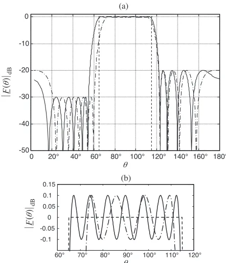
To compare with realpatterns, let us consider a flat-toped beam pattern, defined in the region 65◦ ≤ θ ≤115◦, with 16 elements and
d= λ/2, with a SSL = 20 dB to the left side of the main beam and SLL = 40 dB to the right side, and with a ripple of ±0.1 dB. The presented technique was applied with P = 1024 for the FFT. The result is represented in Figure 1 by the continuous line. To reduce the error below 0.01 dB six iterations for the algorithm were considered. Represented by a dash and a dot line is the result for the approximated real array factor calculated by the method presented in [10]. It was necessary six iterations to produce an error below the referred one. With other examples, it was generally verified that the real pattern requires less iterations than the complex pattern. Furthermore, since in the complex patterns the sample phases must be determined, the computation involved in each iteration takes more time than for real patterns. However, concerning the dynamic range ratio, for the above example the real pattern has a value |Imax|/|Imin| = 34.3, whilst for the complex pattern this relation is only |Imax|/|Imin| = 3.6. It was also verified that the amplitude ratios of the source distribution for the complex pattern varied between 3.6 and 70.5. In Figure 2 is represented the source distribution obtained through the synthesis technique for the best dynamic range ratio.
Another example is the well-known cosec (θ) beam pattern, defined by F(θ) = cosec (θ−π/2), 100◦ ≤ θ ≤ 140◦. For an array with 16 elements and d = λ/2, the ripple should be at ±0.1 dB, the sidelobe level at 20 dB and the first four sidelobes on the left side of the main beam must be 30 dB below the maximum of the function, which is at 100◦. Changing the variable for βz, the array factor becomes
-50 -40 -30 -20 -10 0
0 20° 40° 60° 80° 100° 120° 140° 160° 180°
-0.1 -0.05
0 0.05 0.1 0.15
60° 70° 80° 90° 100° 110° 120° (a)
(b)
θ
θ
( )
|F |dB
θ
( )
|F |dB
θ
Figure 1. Approximated array factor for the flat-topped pattern: (a) complex pattern calculated with the presented technique, represented by the continuous line, and real pattern, represented by the dash and dot line; (b) ripple in the beam zone.
-4λ -3λ -2λ -λ 0 λ 2λ 3λ 4λ 0
0.05 0.1 0.15 0.2 0.25
z
|
c
(
z
)|
-2 0 2
ar
g[
c
(
z
)]
-4λ -3λ -2λ -λ 0 λ 2λ 3λ 4λ z
-40 -35 -30 -25 -20 -15 -10 -5 0
0 20° 40° 60° 80° 100° 120° 140° 160° 180° θ
( )
|F
|dB
θ
Figure 3. Approximated array factor for the cosec (θ) pattern.
-45 -40 -35 -30 -25 -20 -15 -10 -5 0
0 20° 40° 60° 80° 100° 120° 140° 160° 180°
-50
θ
( )
|F |dB
θ
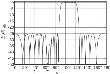
Figure 4. Array factor for the flat-topped pattern with nulls in the positions: θ= 40◦, θ = 64◦ and θ= 66◦.
technique with P = 1024 for the FFT the result is in Figure 3. To produce an error below 0.01 dB, seven iterations were necessary. This result coincides with the one obtained by the Orchard-Elliot technique for the same number of iterations. Therefore, in both techniques the source distribution is similar, which gives the same dynamic range ratio. However, the presented technique is about three times faster than the Orchard-Elliot’s and uses samples of the array factor instead of the indirect controlwith roots around the unit circle.
interval90◦ to 120◦, withN = 21 elements andd=λ/2. The ripple is ±0.2 dB, the SLL = 25 dB and nulls are imposed inθ= 40◦, θ= 64◦ and θ = 66◦. The technique was applied with P = 1024 points for the FFT, with two iterations for the first approximation of the shaped beam pattern and four iterations after the null introduction to produce an error below 0.0005 dB. Figure 4 shows the result. For comparison, if the nulls were imposed in the first iteration, eleven iterations were necessary to reach the same error.
5. CONCLUSION
A new technique that uses efficiently the phase of the array factor was presented. It is considered to synthesize shaped beam patterns with a number of samples of the array factor equal to the number of array elements. The control of the array factor is performed through non-uniformly positions of this function. In previous works where this procedure was used, only the amplitude of the array factor was considered to controlthe pattern. In this work the phase is also used, which permits to increase the number of degrees of freedom. Therefore, a complex pattern is obtained with better characteristics than those of realpatterns. The effectiveness of the presented technique was demonstrated with examples such as flat-top beam patterns and cosec (θ) patterns.
REFERENCES
1. Balanis, C. A.,Antenna Theory, Analysis and Design, 2nd edition, John Wiley & Sons, 1997.
2. Woodward, P. M. and J. D. Lawson, “The theoreticalprecision with which an arbitrary radiation-pattern may be obtained from a source of finite size,” Journal IEE, Vol. 95, No. 37, 363–370, September 1948.
3. Mailloux, R. J., Phased Array Antenna Handbook, Artech House, 1994.
4. Elliot, R. S. and G. J. Sten, “A new technique for shaped beam synthesis of equispaced arrays,”IEEE Transactions, Vol. AP-32, No. 10, 1129–1133, 1984.
5. Orchard, H. J., R. S. Elliot, and G. J. Sten, “Optimising the synthesis of shaped beam antenna patterns,” IEE Proceedings, Vol. 132, Pt. H, No. 1, 63–68, 1985.
7. Hu, J.-L., C. H. Chan, K.-M. Luk, and S.-M. Lin, “Shaped-beam pattern synthesis for base station antenna in mobile communication system,” Microwave and Optical Technology Letters, Vol. 24, No. 4, 226–228, 2000.
8. Shavit, R. and S. Levy, “A new approach to the Orchard-Elliot pattern synthesis algorithm using LMS and pseudoinverse techniques,” Microwave and Optical Technology Letters, Vol. 30, No. 1, 12–15, 2001.
9. Casimiro, A. M. and J. A. Azevedo, “New techniques that unify the procedure of the analysis and synthesis of antenna arrays,”
Journal of Electromagnetics Waves and Applications, Vol. 19, No. 14, 1881–1896, 2005.
10. Azevedo, J. A. and A. M. Casimiro, “Non-uniform sampling and polynomial interpolation for array synthesis,” IET Microw. Antennas Propagat., Vol. 1, No. 4, 867–873, 2007.
11. Azevedo, J. A., “The use of non-uniform sample phases for array synthesis,”15th International Conference on Digital Signal Processing, 95–98, Cardiff, Wales, UK, July 2007.