Prediction Of Effects On Absenteeism Using Hierarchical
Multiple Regression Analysis
Thin Thin San
1, Hlaing Phyu Phyu Mon
2,
War War Myint
3& Zin Mar Naing
41
University of Computer Studies (Meiktila), Faculty of Information Science
2,3,4
University of Computer Studies (Meiktila), Faculty of Information Science
Abstract:
Absenteeism has always been one of the persistent problems in organization. Absenteeism is generally understood in different ways by different persons. It is commonly understood as a staff or a group of staffs remaining absent from work either continuously for a long period or repeatedly for short periods. The study has been conducted to understand the causes for the absenteeism in the company among the staffs using hierarchical multiple regression analysis. Hierarchical Multiple Regression Analysis was used to analyze the absenteeism. The parameters such as demographic characteristics (age, education status, marital status, number of children), service and work attitudes (job satisfaction and organizational commitment) are used to predict the effects of staff’s absenteeism in organization.
Keywords
Absenteeism, hierarchical multiple regression analysis, demographic characteristics
Introduction
Absenteeism is one of the stubborn problems for which there is no clear culprit and no easy cure. , as a general phenomenon it does not discriminate against individuals on the basis of sex, race and religion. Staff attendance is based on a staff’s motivation to attend as well as their ability to attend. A staffs’ ability to attend is influenced by factors such as family responsibilities, transportation problems, accidents and so on. Once all these variables are identified, managers may begin to understand why staffs sometimes choose not to come to work when they are fully capable of attending. Work-related commitments can increase performance, reduce absenteeism and benefit both the staff and the organization.
Absenteeism is commonly understood as an staff or a group of staffs remaining absent from work either continuously for a long period or repeatedly for short periods [8]. Basically absence can be divided into an involuntary part and a voluntary part. Involuntary part e.g. certified sickness, funeral attendance, public holiday, casual leave, maternity
leave or force majeure, is beyond the staff’s immediate control. In this paper, Absenteeism is measured by the number of workdays that is taken off. It is defined as leave without pay, unscheduled absence from work, regardless of the reason, including long and short term disability.
Hierarchical multiple regression is a type of multiple regression. Multiple regression is an extension of simple linear regression. It is used when we want to predict the value of a variable based on the value of two or more other variables. In this paper, independent variables are demographic characteristics, service, work attitudes and absenteeism is dependent variable. .
Hierarchical multiple regressions is used to evaluate the relationship between a set of independent variables and the dependent variable, controlling for or taking into account the impact of a different set of independent variables on the dependent variable. In order to test the hypothesis suggested, three different regression models are constructed using hierarchical multiple regression analysis. It lets dependent variable y to be modeled as a linear function of, predictor variables or attributes,
A
1,
A
2,
,
A
kdescribing a tuple X. (Thatis, X= (
x
1,
x
2,
,
x
k). The purpose is to predict thevalue of the dependent variable (also referred to as the response variable) using a linear function of the independent variables. The values of the independent variables (also referred to as predictor variables, repressors or covariates) are known quantities for purposes of prediction, the model is:
x x kxk
Y 0 1 1 2 2
(1.1)
Where ε, the “noise” variable, is a normally distributed random variable with mean equal to zero and standard deviation σ and the value of coefficient,
k
0, 1, 2,, whose values are not known. The data consists of n rows of observations also called the cases, which give us values;
ki i
i
i
x
x
x
2
1
2 2 1 1
0 )
(
n
i
k k
i x x x
y (1.2)
Hierarchical multiple regression is applied to study the causes and level of absenteeism among staffs in the company.
2.
Data Mining
Data mining is the task of discovering interesting patterns from large amounts of data, where the data can be stored in databases, data warehouses, or other information repositories and transform it into an understandable structure for further use. Other contributing areas include neural networks, pattern recognition, spatial data analysis, image databases, signal processing and many application fields, such as business, economics and bioinformatics.
The goal of data mining effort can be divided into two different categories: (1) using data mining technique to generate descriptive model to solve problems; (2) using data mining technique to generate predictive model to solve problems. The predictive data mining tasks perform inference of the current data in order to make prediction while the descriptive data mining tasks characterize the general properties of the data in the database. The data mining function, prediction is applied to build effects on absenteeism system using hierarchical multiple regression analysis which is the most popular and is often used to test the hypothesis suggested by a number of factors.
.
2.1 Regression Model
The regression model is a statistical procedure that allows estimating the linear or straight line, relationship that relates two or more variables. This linear relationship summarizes the amount of change in one variable that is associated with change in another variable or variables. The model can also be tested for statistical significance, to test whether the observed linear relationship could have emerged by chance or not. In statistical methods, multivariate regression with relationships among several variables is examined. The regression model assigns one of the variables the status of an independent variable and the other variable the status of a dependent variable. The independent variable may be regarded as causing changes in the dependent variable, or the independent variable may occur prior in time to the dependent variable.
.2.1.1 Hierarchical Multiple Regression Analysis
The hierarchical multiple regression equation is an expansion of the equations for the multiple regressions. Multiple regression analysis is a
powerful technique used for predicting the unknown value of a variable from the known value of two or more variables also called the predictors. More precisely, multiple regression analysis helps us to predict the value of Y for given values of
1
X, X2,….,
k X .
By multiple regressions, the variable whose value is to be predicted is known as the dependent variable and the ones whose known values are used for prediction are known as independent variables. Multiple regression model is as follows:
y'b0b1x1ib2x2ib3x3i...bkxk (2.1) In this model, y = A predicted value of Y
(which is depending variable), b0= the value of Y when X is equal “zero”. This is called the “Y Intercept”. b1=the coefficient of
1
x
b
2= coefficient of2
x and so on.
x
1,x
2=predictor variables.2.2 Ordinary Least Squares
Ordinary Least Squares (OLS) or linear least squares is a method for estimating the unknown parameters in a regression model. OLS chooses the parameters of a linear function of a set of explanatory variables by minimizing the sum of the squares of the differences between the observed dependent variable (values of the variable being predicted) in the given dataset and those predicted by the linear function. OLS is to closely fit a function with the data.
The least squares estimates of the coefficients
k
1, 2,, are the valuesb0, b1,…,bk for which the
sum of squared errors, SSE is a minimum.
2
1
2 2 1 1
0 )
(
n
i
k k
i b bx b x b x
y
(2.2) The coefficient estimators are computed using the following equation:
b XX Xy 1
)
( (2.3)
2.3 Sum-of-Squares Decomposition
The model variability can be partitioned into the components
SST
= SSR +SSE
n i1Yi Y
2 )
( = n
i1Yi Y
2
) '
( +
n i1Yi Yi
2 ) ' (
(2.4)
2.3.1 Sum-of-Squares Regression
The sum of squared regression measures how much of the variation in the dependent variable the model.
SS
Regression =
n i1 Yi Y
2 ) '
2.3.2 Sum-of-Squares Residual
The sum of squared error is used to decide if a model is a good fit for the observed data. It measures the overall difference between data and values predicted by estimation model.
SS
Residual=
n
i1 Yi Yi 2
) '
( (2.6)
2.3.3 Sum-of-Squares Total
The sum of squares total represents a measure of variation or deviation from the mean. It is calculated as a summation of the squares of the differences from the mean.
SST
=
n i1Yi Y2 )
( (2.7)
2.4 Mean Squared Regression and Residual
The mean squared regression is computed by dividing SSR by a number referred to as its degrees of freedom.
MSR
=k
SSR (2.8)
The mean squared residual measures the average of the squares of the errors that is, the difference between the estimator and what is estimated. It is computed by dividing by its degrees of freedom. It is always non-negative, and values closer to zero are better.
MS
Residual =1
Re
k
n
SS
sidual
(
2.9
)2.5 Hypothesis Testing
In regression hypothesis testing the difference is most prominent. The hypothesis is a simple proposition that can be proved or disproved through various scientific techniques and establishes the relationship between independent and some dependent variable.
Testing of a hypothesis attempts to make clear, whether or not the supposition is valid. T-statistic is used to test the significance of individual coefficients and F-statistic is used to test the overall significance of the model. F-test in regression compares the fits of different linear models. Unlike t-tests that can assess only one regression coefficient at a time, the F-test can assess multiple coefficients simultaneously.
F =
sidual MS
MSR
Re
(2.10)
where, F = F- test,
MSR = mean squared regression,MSResidual = mean
squared residual
2.6 Correlation Analysis
Correlation analysis is a method that is used to study the strength of a relationship between two, numerically measured and continuous variables. It is useful when we want to establish if there are possible connections between variables. If there is correlation found, depending upon the numerical values measured, this can be either positive or negative.
The ratio of the sum of squares regression, SSR, divided by the total sum of squares,
SST
, provides a descriptive measure of the proportion, or percent, of the total variability that is explained by the regression model. This measure is called the coefficient of determination, 2R .
2
R =
SST SSR= 1-
SST
SSE (2.11)
2.7 Standard Error and Descriptive Statistics
The standard error is an important indicator of how precise an estimate of the population parameter the sample statistic is. The term standard error refers to a group of statistics that provide information about the dispersion of the values within a set. When the standard error is large relative to the statistic, the statistic will typically be non-significant.
Descriptive Statistics are used to describe the basic features of the data in a study. They provide simple summaries about the sample and the measures. Descriptive statistics help us to simply large amounts of data in a sensible way. Each descriptive statistics reduces lots of data into a simple summary. The major types of descriptive statistics are mean, variance and standard deviation
3.
.Implementation
The main objective of this system is to analyze the relationship between demographic characteristics, service work attitudes and absenteeism. The current study employed prediction of effects on absenteeism in order to test the hypothesis suggested on staff’s absenteeism in company. The absence data is used in this project is 148 staffs in ABC Company, 68 staffs in Company department and IBM human resource dataset.
variables (age, educations status, marital status, number of children) were entered into equation. In the second model, demographic variables and service were entered.
Models were tested by comparing a model with no predictors to the model that specify. Later, hypothesis testing was conducted to determine which hypothesis proposed based on this study are strongly supported. The system flow diagram of the system is shown in Figure 3.1.
Figure 3.1 System Flow Diagram Using F-Test
3.1 Data Analysis Process
The data about the demographic characteristics and service of staffs were taken from the human
resources department. Education status is defined as high school = 1, bachelor = 2, honours = 3 and master = 4. Marital status is defined as a dichotomous variable (married = 1, single = 0).
3.1.1 Demographic Characteristics and Work Attitude’s Measurement
Prediction of effects on absenteeism system contains different personal and demographics information such as age, education status, marital status, number of children and service are presented in Table 3.1.
Table 3.1 Demographic Characteristics of Participants
Variable Category Frequency Percent
Age 19-30 Years 31-55 Years
115 33
77.7 22.3 Education
Status
Master’s degree Honor’s degree Bachelor’s degree Others
5 7 107 29
3.4 4.7 72.3 19.6 Marital
Status
Married Single
70 78
47 53 Number
of Children
1-2 Children 3-4 Children Others
43 6 99
29.1 4.1 66.8 Service 1-10 Years
11-24 Years
131 17
88.5 11.5
Demographic characteristics showed that the majority of the characteristics (77.7 %) fall in the age range between 19 to 30 years of age. Most of the them are having Bachelor’s Degree (72.3 %). Additionally, while (48 %) of staffs are married, (34.5 %) of staffs have children. On the other hand, most of the staffs (88.5 %) are there in the range between 1 to 10 years of service.
3.2
Hierarchical Multiple Regression
Analysis
The results of hierarchical regression analysis that are used to test the hypothesis are shown in Tables. Three models were tested separately. In the first model, only the demographic characteristics of workers; in the second model, both the demographic characteristics and service; in the third model, demographic characteristics, service and work attitudes being worked were taken as variables of the system. This approach makes the comparison of subjective influences of each of 3sets of variables on the variant, possible. The general form of hierarchical multiple regression is
4 4 3 3 2 2 1 1
0
b
x
b
x
b
x
b
x
b
y
YESNO Start
Compute correlation coefficients by OLS
Calculate predicted absenteeism by multiple
regression analysis
Calculate SSRegression ,
SResidual and SSTotal
Calculate the F-test based on
MSRegression and MSResidual
Accept
End Load data set for each
Model
If F> Kf ? Reject Staff’s
Demographic
Characteristics Absenteeism
Figure 3.2 Model 1
4 3
2
1 0.565 2.086 0.190
010 . 0 081 .
4 x x x x
y
where, y = absenteeism,
1
x
= age,x
2= education status,x
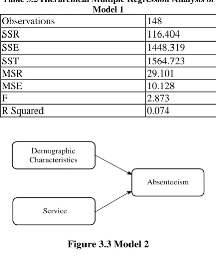
3= marital status and x4= no. of childrenTable 3.2 Hierarchical Multiple Regression Analysis of Model 1
Observations 148
SSR 116.404
SSE 1448.319
SST 1564.723
MSR 29.101
MSE 10.128
F 2.873
R Squared 0.074
Demographic Characteristics
Absenteeism
Service
Figure 3.3 Model 2
5 4
3 2
1
0
.
599
2
.
061
0
.
107
0
.
083
042
.
0
925
.
2
x
x
x
x
x
y
where, y = absenteeism,
1
x
= age,x
2= education status,x
3= marital status,4
x
= no. of children and 5x = service
Table 3.3 Hierarchical Multiple Regression Analysis of Model 2
Observations 148
SSR 121.260
SSE 1443.463
SST 1564.723
MSR 24.252
MSE 10.165
F 2.386
R Squared 0.077
Table 3.4 Critical Value of Model with α = 0.05
Model 1 Model 2
Critical Value 2.435 2.277
The coefficient of determination 2
R (2.11) of Model 1 was 7.4%, Model 2 was 7.7%. Each model analyzed step by step and hypothesis testing was conducted to determine which hypothesis proposed based on this study are strongly supported.
3.3 Hypothesis Testing
Regression estimates of Model 1 shows that the demographic characteristics found significantly linked with absenteeism. There is a significant positive relationship between demographic characteristics and absenteeism with (F = 2.873) and ( critical value = 2.434). Demographic character- istics explained 7.4% of variant on absenteeism. This result of the study support Model 1.
In the model 2, there is a significant positive relationship between demographic characteristics, service and absenteeism with (F = 2.386) and ( critical value = 2.277). Demographic characteristics and service explained 7.7% of variant on absenteeism. Based on this result, Model 2 can be accepted.
Table 3.5 Hypothesis Testing Results of Model with α = 0.05
Model F-Value Significance
Testing (95%)
Results
Model 1 2.873 F 2.434 Accepted
Model 2 2.386 F 2.277 Accepted
3.4 Regression Coefficient
Model 1 (Demographic Characteristics) , Model 2 (Demographic Characteristics and Service) were chosen to prove the hypotheses that strongly significant effects on absenteeism.
Table 3.6 Regression Results of Model 1 with α = 0.05
Variable Coeffi
cients
Stand--ard Error
T-Test
Significa-nce Testing
(95%) Resu
-lts
Age -0.010 0.062 -0.163 0.163 1.976
Not Acce pted Education
Status
0.565 0.453 1.247 1.247 1.976
Not Acce pted Marital
Status
2.086 0.702 2.972 2.972 1.976
Number of Children
-0.190 0.480 -0.397 0.397 1.976
Not Acce pted
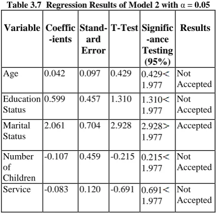
Table 3.7 Regression Results of Model 2 with α = 0.05
Variable Coeffic
-ients
Stand-ard Error
T-Test Signific
-ance Testing
(95%)
Results
Age 0.042 0.097 0.429 0.429 1.977
Not Accepted
Education Status
0.599 0.457 1.310 1.310 1.977
Not Accepted
Marital Status
2.061 0.704 2.928 2.928 1.977
Accepted
Number of Children
-0.107 0.459 -0.215 0.215 1.977
Not Accepted
Service -0.083 0.120 -0.691 0.691 1.977
Not Accepted
Table 3.6 and Table 3.7 show that marital status towards absenteeism was strongly related at T-Test 1.976 and T-Test 1.977. The coefficient of determination 2
R of marital status in Model 1 was 44.2% and Model 2 was 44.3%. This means that marital status contributes towards absenteeism.
3.5 Experimental Results
The results of IBM dataset shows significant relationship between service year, job satisfaction and absenteeism with significant level α = 0.01, α = 0.05 and α = 0.1. This data was taken from IBM Human Resource Department which was transformed hourly rate to daily rate as absence day. Based on this data, hypothesis of service year was strongly accepted. Most of the staff are there in the range one year of service, while the staff with 40 years of service is highest and the least service is less than one year. When analysis of service year and absence on each staff, one year of service staff was taken more absence than 40 years of service staff . According to the test result on each staff , the staff with low service will have significantly linked with higher absenteeism.
4.
Conclusion
The aim of this system is to understand prediction of effects on absenteeism system. Absenteeism rates of staffs working in ABC Company have been examined and factors that might
cause absenteeism have been investigated with the help of hierarchical multiple regression analysis. According to the results of hierarchical multiple regression analysis, the results obtained helps to verify the established hypothesis and to understand the relationship of the six variables with absenteeism. The finding reveals that age, education status, marital status, number of children, service and organizational commitment are the factors that affect absenteeism. Surprisingly, the effect of job satisfaction was not significant on absenteeism.
This study has determined the overall absenteeism rate, the various factors influencing absence rates. Creating a better physical working environment, reduction of stress among staffs can be achieved by improvement in the manager or supervisor-worker and worker-worker relationships. Providing incentives for reduced absenteeism among staff could help in motivating them to avoid unnecessary absenteeism.
5.
Acknowledgements
I would like to express my special thanks to all my teachers who gave me their time and guidance, and all my friends who helped in the task of developing this paper. Finally, I would like especially to thank my parents for their continuous support and encouragement throughout my whole life.
6. References
[1] Atang Azael Ntisa. Job Satisfaction, Organizational Commitment, Turnover Intention, Absenteeism and Work Performance Amongst Academics Within South African Universities of Technology
[2] Beverley Ann Josias. The relationship between job satisfaction and absenteeism in a selected field services section within an electricity utility in the western cape
[3] Chapter 5A:Multiple Regression Analysis- Sage Publications
[4] Cohen, A., & Golan, R. (2007). Predicting absenteeism and turnover intentions by past absenteeism and work attitudes: An empirical examination of female employees in long term nursing care facilities. Career Development
International, 12(5), 416-432.
[5] Derivation of the Least Squares Estimator for Beta in Matrix Notation
[7] John V.Petrocelli. Hierarchical Multiple Regression in Counseling Research: Common Problems and Possible Remedies
[8] Murthy, S.A.S., (1954): A study on absenteeism, Abhinav Journal of Social Work, 14 (1-4), P.132.
[9] Paul Newbold, William L. Carlson & Betty M. Thorne Statistics for Business and Economics. 8th ed. (ISBN 13:978-0-13-2745659)
[10] Richard T. Mowday And Richard M. Steers, Lyman W. Porter. The Measurement of Organizational Commitment, Journal of Vocational Behavior 14, 224-247 (1979) [11] Tekin Akgeyik, Istanbul University, Istanbul,
Turkey. Factors affecting employee absenteeism* (A study on a sample of textile workers), European Journal of Management, V.14 (3), 2014: 69-76.
[12] William T. Hoyt, Stephen Leierer and Michael J. Millington. Rehabil Couns Bull 2006; 49; 223, Analysis and Interpretation of Findings Using Multiple Regression Techniques
[13] http://uregina.ca/~gingrich/regr.pdf
[14]https://onlinecourses.science.psu.edu/statprogra m/reviews/statistical-concepts/hypothesis-testing/critical-value-approach
[15] https://www.citehr.com/309682-job-satisfaction-questionnaire.html