Laporte, Chervin F. P. (2014): Evolution of clusters and large-scale structures of galaxies. Dissertation, LMU München: Fakultät für Physik

(1)

Evolution of clusters and large-scale

structures of galaxies

Chervin F. P. Laporte

(2)

(3)

Evolution of clusters and large-scale

structures of galaxies

Chervin F. P. Laporte

Dissertation

an der Fakult¨

at f¨

ur Physik

der Ludwig–Maximilians–Universit¨

at

M¨

unchen

vorgelegt von

Chervin F. P. Laporte

aus Versailles, Yvelines, France

(4)

(5)

List of Figures

1.1 CMB Planck 2013 Map . . . 6

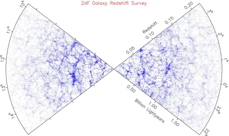
1.2 Large Scale Structures: 2FGRS . . . 6

1.3 Thermal History of Universe . . . 14

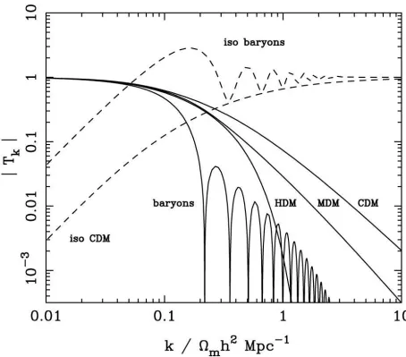
1.4 Transfer Functions . . . 15

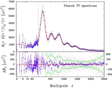
2.1 Temperature Power Spectrum as measured by Planck 2013 . . . 19

2.2 Cold Dark Matter vs. Hot Dark Matter & the CfA survey . . . 20

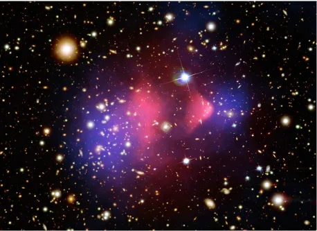
2.3 The Bullet Cluster . . . 22

3.1 Barnes & Hut 1983: Oct-Tree illustration . . . 25

3.2 Cosmological N-body simulations: The Millennium run . . . 29

4.1 Differential energy distributions for rescaled galaxies . . . 37

4.2 Density profiles of rescaled galaxies . . . 38

4.3 Normalised radial stellar mass distribution in BCG atz = 0 . . . 43

4.4 Total and dark matter slopes for original runs and rescaled versions. . . 45

5.1 Triaxial tracer weighting scheme: example density profile . . . 53

5.2 Triaxial tracer weighting scheme: stability test . . . 54

5.3 Stellar-to-halo mass relations at z = 2 and z = 0: BCGs and cluster ellipticals 56 5.4 z = 0 surface brightness profiles of BCGs . . . 57

5.5 z = 1 surface brightness profiles of BCGs . . . 59

5.6 Stellar density profiles of BCGs: in-situ, accreted and total . . . 60

5.7 BCG cluster mass evolution: z = 1, z = 0.3 andz = 0 . . . 62

5.8 Mass-size evolution for cluster galaxies: z = 2, z = 1, z = 0.3 and z = 0 . . 64

6.1 Stability test: stellar density profile evolution . . . 72

6.2 Stability test: stellar, dark and total density profile . . . 73

6.3 Stability test: x-y projection of stars . . . 74

6.4 The z = 2 mass-size relation . . . 75

6.5 Distribution of central z = 0 10 kpc DM particles at z = 2 . . . 77

6.6 Final density profiles for stars, dark matter and total matter. . . 78

(10)

x Abbildungsverzeichnis

(11)

List of Tables

4.1 Rescaled simulations: size and stellar mass growth factors . . . 42

5.1 BCG stellar mass accretion . . . 63

5.2 BCG merger counts . . . 65

6.1 Phoenix Clusters Properties . . . 76

(12)

(13)

Zusammenfassung

Diese Doktorarbeit befasst sich mit der Bildung und Entwicklung der Hellsten Haufen-galaxien (Brightest Cluster Galaxies, BCGs) und mit der zentralen Verteilung von Dunkler Materie (DM) in Galaxienhaufen in kosmologischen N-Körper Simulationen im Rahmen des ΛCDM Paradigmas. Dabei werden folgende Fragen behandelt: Wachsen BCGs durch dissipationsfreie Merger innerhalb der letzten 10 Gigajahre? Wenn ja, was sind ihre struk-turellen Eigenschaften? Sind die vorhergesagten Massenwachstumsraten der BCGs in den letzten 10 Gigajahren in Übereinstimmung mit Beobachtungen? Welche Bedeutung hat die dissipationsfreie Bildung von BCGs für die zentrale Verteilung der DM in Galaxienhaufen? Legen die Beobachtungsdaten der Verteilung der DM in Galaxienhaufen tatsächlich nahe, dass die Vorstellung der DM als kalt und kollisionsfrei überdacht werden muss?

Die ersten drei Kapitel dieser Arbeit geben einen Überblick über Kosmologie, Struktur-bildung, die Natur der Dunklen Materie und über numerische Techniken in kosmologischen N-Körper Simulationen.

In Kapitel 4 wird anhand eines Sets von kosmologischen N-Körper Simulationen und mehreren reskalierten Versionen dieser Simulationen untersucht, wie sich zentral schwach konzentrierte Verteilungen von Dunkler Materie (shallow DM cusps) durch dissipations-freie Verschmelzungen von Galaxien (Merger) bilden können. Es wird die Abhängigkeit der Mischung von DM und Sternen im Zentrum der Haufen zu späteren Zeiten von der ursprünglichen stellaren Struktur untersucht. Es stellt sich heraus, dass qualitativ flache DM cusps im Zentrum von Galaxienhaufen natürlicherweise zu erwarten sind, falls die Bildung der BCGs in erster Linie durch dissipationsfreie Merger abläuft.

In Kapitel 5 wird ein allgemeines Gewichtungsschema entwickelt, um Gleichgewichtsverteilungs-funktionen der Form f(E) in triaxialen Potentialen zu generieren. Dieses Schema wird

(14)

vorher-xiv Zusammenfassung

sagt, und zwar mit der Häufigkeit und Massenverteilungsrate, die benötigt wird, um die beobachteten Wachstumsraten von passiven Galaxien seit z = 2 zu erklären.

In Kapitel 6 wird die Frage nach der Verteilung der DM im Zentrum von Haufen-galaxien wieder aufgegriffen. Es wird eine Methode entwickelt, um selbst-gravitative Gle-ichgewichtverteilungsfunktionen in die in den kosmologischen Simulationen gebildeten DM Halos einzufügen.Es stellt sich heraus, dass das Gesamtdichteprofil unter Hinzunahme von Baryonen bei z = 2 durch die hohe Zahl an Mergern im Zentrum von Haufengalaxien wieder nahe an dem der ursprünglichen reinen DM Simulationen liegt (mit Ausnahme der innersten Bereiche, _∼ 5 kpc). Diese Ergebnisse legen die Existenz einer Attraktor-Lösung für kollisionsfreie Systeme nahe, ungeachtet der Hinzunahme von Baryonen, bei denen Mischvorgänge effektiv sind. Die Dichteprofile von DM in den Resimulationen sind flacher als die in den reinen DM Simulationen mit einem Unterschied von ∆γ _≡∆(d_dln_lnrρ)_∼ 0.3₋0.4. Die Skala, auf der dieser Übergang geschieht, ähnelt der von Beobachtungen um r/r200 ∼ 0.01−0.02 suggerierten Skala. Es wird außerdem vermutet, dass der

Ef-fekt der Erhitzung durch dynamische Reibung von einfallenden Schwarzen Löchern die weitere zentrale Massenverteilung innerhalb von r_∼5 kpc beeinflussen kann. Die berech-neten Massendefizite könnten eine natürliche Erklärung für einige der größten zentralen Sternkonzentrationen innerhalb vonrc ∼3 kpc darstellen, die in BCGs beobachtet werden.

(15)

Summary

(16)

xvi Zusammenfassung

density profile back to a solution closely resembling that of the original dark matter only runs (except in the inner-most regions below 6₋4 kpc). This suggests the existence of an attractor solution for collisionless systems, irrespective of the baryonic loading where mixing is effective. The dark matter density profiles in these re-simulaitons as a result are shallower than those in the dark matter only runs with a difference of ∆γ _∼0.3₋0.4. The scale at which the transition occurs is exactly similar with that inferred by observations around r/r200 ∼ 0.01− 0.02. We further estimate that the effect of dynamical friction

heating impeded by infalling black holes can affect further the central mass distribution belowr _∼4₋6 kpc. Our calculated mass-deficits would provide a natural explanation for some of the largest stellar cores ofrc ∼3 kpc observed in BCGs. The final part of the thesis

(17)

Part I

(18)

(19)

3

Pour Marie-Am´elie Laporte (1956-2012), To my cousin Pierre Demarque,

(20)

(21)

Chapter 1 Background Cosmology & Structure

Formation

While it is difficult to give a rigorous overview of all subfields of astrophysics that make the basis of this thesis - this should be the topic of a textbook - I shall discuss a few selected salient aspects of physics which form the backbone to understanding structure formation in its full cosmological context. I shall focus more specifically on our currently most favoured cosmological model, the ΛCDM paradigm which is at the heart of the work presented in this thesis. In passing, I will point out the relevant references which go in further details on each subject.

1.1 Background Friedman Robertson-Walker

Cosmol-ogy

The description of the standard cosmological model is based on two fundamental observa-tions about the Universe. Firstly, on large scale the Universe ishomogeneousandisotropic. That is to say, there is no preferred observing position and the Universe looks the same in every direction. This is the Copernican principle. Second, space expands such that the physical distance between any two fundamental observers (i.e. one at rest with respect to the matter field around it) must have the form:

r=xa(t), (1.1)

where we have introduced the scale factor which connects co-moving coordinate x to the physical one r. This is known as Hubble’s law of expansion.

Observation of the Cosmic Microwave Background (CMB) confirm homogeneity to the level of ∆T

T ∼ O(10

−5_{) (Smoot et al., 1992). This is shown in Figure 1.1. Observations of}

the large scale structures (LSS) also confirm isotropy when smoothing the density field on scales of 100h−1_{Mpc (Figure 1.2).}

(22)

6 1. Background Cosmology & Structure Formation

Figure 1.1: Cosmic Microwave Background from the Planck 2013 collaboration. The tem-perature fluctuations are so small ∆T

T ∼ O(10

−5_{), supporting the idea that the Universe is}

homogeneous on large scales.

(23)

1.1 Background Friedman Robertson-Walker Cosmology 7

gµν for which the line element is:

ds2 ₌_g

µνdxµdxν. (1.2)

The most general metric for an isotropic and homogeneous Universe is given by the Robertson-Walker metric:

ds2 =c2dt2₋a2(t)

dr2

1₋kr2 +r

2₍_dθ2₊_sin2_φ2₎

, (1.3)

where (r, θ, φ) are comoving coordinates in spherical coordinates (i.e., r2 ₌_x2 ₊_y2₊_z2₎

and k is the spatial curvature (which can take values of -1, 0 and 1).

The equations governing the evolution of the Universe can be derived by manipulating the Einstein field equation:

Rµν−

1

2gµνR−gµνΛ = 8πG

c4 Tµν, (1.4)

Where Tµν is the energy momentum tensor, R the curvature scalar and Rµν the Ricci

tensor.The Ricci tensor and curvature scalar can be calculated from the metric. For a perfect fluid (one with no viscous stress), the energy-momentum tensor is entirely specified by the rest frame densityρand isotropic rest frame pressureP and soTµν is diagonal. The

general form in any frame is given by:

Tµν = (ρ+P)UµUν +P gµν (1.5)

For a uniform ideal fluid in the rest frame this reduces toTµν = diag(ρ,−giiP). Solving

for the 00 and ii components one recovers two equations fully specifying the evolution of

the cosmological background.

These are the Raychaudhuri equation

¨

a a =−

4πG

3

ρ+ 3P

c2

+Λc

2

3 (1.6)

and the Friedmann equation

˙

a a

2

= 8πG 3 ρ−

kc2

a2 +

Λc2

3 . (1.7)

Observations of the CMB and the LSS find that the Universe is flat and composed of radiation, matter (in the form of baryons and dark matter) and dark energy (represented by a cosmological constant Λ) causing an accelerated rate of expansion at late times.

The Pressure term can be written in a general form P = wρc2_{. Substituting this into}

the continuity equation we see that the density evolves as:

(24)

Substituting ρinto the Friedmann equation gives the evolution of the scale factor with time:

a_∝t2/3(1+w),_∀w₆=₋1 (1.9)

We now need to define some quantities.

Hubble parameter: This defines the expansion rate of the Universe H(t) = a˙

a. The

expansion rate at the present time is the Hubble constant H(t0) =H0 = 100hkm/s/Mpc,

where h is a dimensionless number (h_∼0.7).

Redshift: As a consequence of the expansion of the Universe, light signals (which follow null geodesicsds= 0) get cosmologically redshifted. We define redshift as 1+z _≡ λ0

λe = a(t0)

a(te),

where λ0, λe,a(t0),a(te) are the wavelengths and scale factors of the light as observed by

an observer today and at emission respectively. In cosmology we generally normalise the scale factor such that at the present time a(t0) = 1. This gives the following relation for

redshift 1 +z =a−1_{. Redshift can also be translated into time due to its dependence on}_a_.

Density parameter: This defines the energy density of all constituents in the Universe Ω = 8πG

3H2ρ=

ρ

ρcrit, where ρcrit is the critical density of the Universe and changes with time

due to its dependency on the Hubble parameter.

Thus we can re-write the Friedmann equation as:

Ω(a)−1

−1 = ₋ 3kc

2

8πGρa2 (1.10)

1.1.1 Inflation

When looking at the CMB it is puzzling to see that homogeneity is validated even on patches where according to the classical Big Bang theory there could not have been any causal contacts between them. This is generally referred to as the horizon problem. More-over, when looking at the Friedmann equation (for non-zero matter and radiation content), the value Ω = 1 is an attractor solution when going back at high redshifts. Given the that the Universe is very close to flat (with Ω only deviating mildly from unity) requires great fine-tuning at earlier times. This is called the flatness problem. These problems are solved altogether by invoking a period of accelerated expansion at early times. This is called inflationis generally implemented using a scalar field with special dynamical prop-erties. Because during an accelerated period of expansion, the comoving horizon decreases

(d dt 1 aH

<0) and thus regions which were actually in causal contact can no longer

commu-nicate. One of the most important predictions from inflation is the primordial form of the matter power-spectrum (an important quantity for the study of the growth of structure) for which we quote the final result.

P(k) = Akn, (1.11)

(25)

1.2 A word on thermal history of the Universe 9

during the radiation era. For an account on inflation we recommend the reader the following textbooks (Liddle & Lyth, 2000; Mukhanov, 2005).

1.2 A word on thermal history of the Universe

At early times, during the radiation era, the temperature of the Universe is so high that it consists of a hot plasma of relativistic particles (νe, νe¯, e,e¯) and photons in thermal

equilibrium (e.g. via Compton scattering). This is guaranteed as long as the interaction rate, Γ, of the species with the photon fluid is higher than the expansion of the Universe (i.e. Γ _≫ H ). As the Universe expands the temperature drops, the interaction rate decreases and species gradually come out of equilibrium and decouple from the photon fluid. Eventually, matter-domination takes over and at a temperature of T _∼ 3000K, the photon energies are too low to keep the Universe ionised. This is the time ofrecombination

when the primordial plasma coalesces to produce neutral hydrogen and the mean free path of photons has increased to the size of the observable universe, giving rise to CMB that we can observe today. The physics of this period is generally quite well understood in terms of the thermodynamics and particle physics involved up to a certain point where classical theories break down. Accounts on this can be found in Kolb & Turner (1990). Figure 1.3 shows a timeline summary of the history of the Universe according to the new Planck Collaboration et al. (2013) cosmology.

1.3 Growth of Structure in the linear regime and the

large-scale structures

On scales smaller than 100h−1_{Mpc, the observed Universe is nothing but isotropic and}

homogeneous. The galaxies which trace the matter density field are grouped in clusters, filaments and empty regions known as voids (see Figure 1.2). Growth of structure needs to be seeded by fluctuations in the matter density field ρ(x, t), leading to a density contrast:

δ(x, t) = ρ(x, t)−ρ¯(t) ¯

ρ(t) , (1.12)

where ρ(x, t) is the density field at position xand ρ is the background density.

The primordial fluctuations in the density field are thought to originate from quantum fluctuations (related to Heisenberg’s uncertainty principle) in the very early Universe which later got stretched during inflation giving rise to a Gaussian random density field with a characteristic power spectrum (as discussed in the previous section). This random Gaussian field evolves through the action of gravity and we generally identify two regimes in the growth of perturbations. The linear regime where δ _≪ 1 (i.e. the amplitude of the perturbations are small) and the non-linear one where the δ _≫1.

(26)

per-10 1. Background Cosmology & Structure Formation

turbations in the complex fluid (made up of collisionless dark matter, photons, neutrinos, and collisional baryonic matter) evolve by solving the Boltzmann equation and at different times (radiation domination and matter domination) and taking account of dissipation effects such as Silk damping (the damping of small-scale oscillations in the baryons due to photon diffusion which occurs at decoupling between matter and radiation) and damping from the streaming velocities of collisionless particles (which introduces a cut-off in the power spectrum). The behaviour for the growth of perturbations for each species is dif-ferent on scales outside and inside the horizon and at difdif-ferent epochs (during radiation domination and matter domination). We shall not discuss relativistic perturbation theory but refer the reader to Ma & Bertschinger (1995) which covers this in appropriate details and for two different choices of gauges (synchronous and conformal Newtonian). Instead we shall only quote the final results from such calculations.

It is interesting to note that, the GR solutions are equivalent to the Newtonian treat-ment on scales within the horizon for cold dark matter and baryons after decoupling. Furthermore, in the current cosmological model, the most dominant form of matter is a non-relativistic collisionless fluid (cold dark matter) which is the main actor in structure formation so we shall instead spend more time discussing the evolution of this component.

1.3.1 Collisional fluid

Consider a fluid with pressure P, density ρ and velocity field u in an expanding Universe and a potential Φ(x, t). The equations of motion of the fluid are:

Continuity ∂tρ+∇r·(ρu) = 0, (1.13)

Euler ∂tu+ (u· ∇r)u=−

1

ρ∇rP − ∇rΦ, (1.14)

Poisson _∇2rΦ = 4πGρ. (1.15)

If we now work in comoving coordinates x defined as r = a(t)x (the proper velocity

u= ˙r= ˙a(t)x+v, v_≡ax˙), the time and spatial derivatives transform as ∇r→

1

a∇x; ∂ ∂t r→ ∂ ∂t x+ ∂x ∂t

r· ∇x=

∂ ∂t −

˙

a

ax· ∇x. (1.16)

Perturbing ρ, u and Φ about their background values:

ρ_→ρ¯(t) +δρ_≡ρ¯(t)(1 +δ) (1.17)

P _→P¯(t) +δP (1.18)

u_→a(t)H(t)x+v (1.19)

(27)

1.3 Growth of Structure in the linear regime and the large-scale structures 11

If one substitutes these back into the evolution equations of the fluid and keep only the terms up to linear order we obtain the following linearised equations:

∂tδ+

1

a∇ ·v= 0 (1.21)

∂tv+Hv=−

1

aρ∇δP −

1

a∇φ (1.22)

∇2φ= 4πGa2ρδ¯ (1.23)

If we now take the time derivative of the perturbed continuity equation and combine it with the perturbed Euler and Poisson equations we obtained the fundamental equation for the growth of structure in Newtonian theory, which illustrates the competition between infall by gravitational attraction and pressure support:

∂2_tδ₋2H∂tδ−4πGρδ¯ −

1

a2_ρ_¯∇

2_δP _{= 0} _(1.24)

If we additionally consider a barotropic fluid (P = P(ρ)) then δP = ∂P_∂ρρδ¯ and if we Fourier expand so that _∇2 _{→ −}_k2 _{we arrive at:}

¨

δk+ 2Hδ˙k+ (

c2

sk2

a2 −4πGρ¯)δk = 0 (1.25)

This is the equation for a damped oscillator provided that c2sk2

a2 >4πGρ¯, giving rise to

acoustic oscillations in the fluid. Forc2

sk2/a2 <4πGρ¯the system is unstable and undergoes

gravitational collapse. The characteristic scale of importance here is the Jeans length

λJ ≡

2πa kJ

=cs

r

π

Gρ¯, (1.26)

which is the distance a sound wave can travel in a gravitational free-fall time. Only perturbations with k < kJ can grow.

The equivalent equation for a collisionless collisionless fluid with no velocity stress reduces is equivalent to that of a collisional fluid with zero pressure. Thus the equation governing the growth of perturbations for dark matter in the linear regime is the same as that for the baryons but omitting the pressure term. The fluid treatment for dark matter becomes invalid in the regime where the velocity dispersion of the collisionless gas is non-negligible and the particles can stream away. In those instances one needs to follow the evolution of the full distribution function (using perturbation theory). This will not be discussed here but the reader can find a discussion in Ma & Bertschinger (1995).

(28)

• radiation domination era inside the horizon: Cold dark matter grows δ _∝

log(t). This growth is due to the effect of radiation causing a more rapid expansion, slowing down the growth of dark matter perturbations (Meszaros effect). Baryons and radiation are still in the tight coupling regime thus δb ∝δr and baryons undergo

acoustic oscillations.

• baryon decoupling/ recombination inside the horizon: Cold dark matter grows as δc ∝ t2/3 as the Universe is very close to an Einstein de Sitter spacetime.

Baryons are no longer coupled to radiation, thus they are able to catch up with cold dark matter.

1.4 Growth of matter and dark matter perturbations

after recombination

After matter-radiation equality, on scales of cosmological interest which are larger than the Jeans scale of baryons, both fluctuations in CDM and the baryons have the same dynamical equation. Quickly after recombination, the overdensity in baryons δb follows

that of cold dark matterδc and the matter behaves as a single collisionless fluid for which

δm = ρ¯b_ρδ_¯b_b+¯_+¯ρ_ρ_ccδc ≈ δc. Furthermore the Universe in this regime is close to an Einstein

de-Sitter Universe (with zero curvature and no dark energy terms). In this case the perturbation growth equation can be simplified to

¨

δm+

4 3tδ˙m−

2

3t2δm = 0, (1.27)

where we used the facts thatH2 _∝_ρ_¯_∝_a−3_,_a_∝ _t2/3 _so _H _{= 2}_/₍₃_t_{) and 4}_πG_ρ_¯_{= 2}_/₍₃_t2_).

If we try solutions of the formδ_∝tβ_{, we find that this equation admits two independent}

solutions: a growingD+ ∝t2/3 and decaying modeD− ∝t−1, thus general solution is given

by their linear combination:

δm =AD+(t) +BD−(t), (1.28)

where A and B are constants. The growing modes eventually take over the decaying ones and we can write the solution as δ _∝D+(t) =D(t). For a general cosmology, the growing

mode is given by:

D(t) =H(t)

Z t

0

dt′

a2₍_t′₎_H2₍_t′₎ =H(t)

Z a

0

da

˙

a3 (1.29)

1.4.1 Primordial Power spectrum and its relation to the

Post-recombination one

(29)

post-1.4 Growth of matter and dark matter perturbations after recombination 13

recombination era. One thus needs to relate the history of the growth of the perturbation of all modes to the time of post-recombination. This can be all encapsulated in the transfer function T(k) which relates the power spectrum in the post-recombination era to that of initial conditions from inflation. In a way, the T(k) contains all of the relevant physics of the early Universe which affected the primordial density field δi(x).This is given by

P(k, t) = _h|δ(k, t)δ∗₍_k′_{, t}₎

|i=Pi(k)D(t)2T2(k, t) (1.30)

(30)

(31)

1.4 Growth of matter and dark matter perturbations after recombination 15

(32)

(33)

Chapter 2 Dark Matter

The most abundant form of matter in the Universe is dark matter. It is thought to be a collisionless fluid that comes out as non-relativistic at the time of decoupling and that interacts only with ordinary matter solely through the force of gravity. In this section we give a brief account of the observational evidence on different scales in support for dark matter. We then discuss the motivations behind why this component cannot be baryonic (the best evidence comes from a cosmological stand point) and introduce the idea of cold dark matter that is at the heart of the standard cosmological model. We then close this section by introducing the principal candidates beyond the standard model that have been proposed by particle physics to account for the dark matter and currently ongoing experiments.

2.1 Observational evidence

2.1.1 Galactic scales

On galactic scales, the evidence for dark matter first came from the observation of rotation curves of spiral galaxies (e.g. (Rubin & Ford, 1970)). These measure the circular velocity of galaxies as a function of radius using optical long-slit spectroscopy or the Doppler shift from the HI 21cm hyperfine transition line associated with the neutral hydrogen gas which extends much further than the optical part traced by the stars. Such measurements have now been performed for a large amount of objects and they all exhibit the same unexpected behaviour: they are flat beyond the edge of their exponentially falling stellar disks. According to Newtonian gravity the circular velocity of a spherical system is defined as v(r) = p(GM(r)/r), where M(r) is the enclosed mass within radius r. Outside the stellar disk,M(r) is expected to be constant (the neutral gas is not self-gravitating and thus counts as a tracer of the underlying potential), thus circular velocity should follow a Kepler falloff v(r) _∝ 1/p(r). If Newtonian gravity is correct, then the flatness of these curves imply that galaxies must be surrounded by extended dark matter haloes with M(r) _∝ r

(34)

18 2. Dark Matter

Strong lensing in galaxies also another manifestation in support for dark matter. In general relativity, light follows null geodesics and gets bent by mass. The projected visible mass density in the plane of a galaxy is negligible to create large deflection angles at the positions where multiple images and arcs appear in lensing galaxies. The multiple images and arcs that are seen around some massive elliptical galaxies or in galaxy clusters imply that the total projected surface density is much higher than that of the stars. In the case, when a galaxy sits directly behind another, this configuration creates an Einstein ring. This feature can be explained to first order if one models the matter distribution as a singular isothermal sphere, where ρ _∝ r−2 _{(note these have also the same property as}

to produce flat circular velocity curves with M(r) _∝ r). Many lenses have been studied showing clear evidence for more matter surrounding galaxies beyond their optical radius.

2.1.2 Galaxy Cluster scales

Already in the 30s, Zwicky (1933) reported the need for dark matter to explain the mass of the Coma Cluster . Using its member galaxies in combination with the virial theorem, he estimated the total mass of Coma and noted that the inferred total mass was factor of 400 off compared to the sum of all the visible light in the cluster galaxies. He later concluded that this dark matter could be observed with the aid of gravitational lensing (Zwicky, 1937). Fritz Zwicky was clearly ahead of his time and it took about 40 years for the idea of dark matter to be really seriously considered by astrophysicists. Nowadays galaxy clusters offer us a great number of probes for studying in detail their total matter content as well as their dark matter content: stellar kinematics from the central galaxies, strong and weak lensing, X-ray emission from the hot electron gas in hydrostatic equilibrium, the motion of satellite galaxies. These various independent probes for mass give all similar answers when compared to each other, providing clear evidence that dark matter dominates the mass budget of galaxy clusters out to large radii (_∼3Mpc)

2.1.3 Cosmological scales

Existence for (non-baryonic) dark matter is now also required from a cosmological point of view. Detailed studies of the cosmic microwave background (CMB), in particular of its angular temperature power spectrum can put strong constraints on the cosmological parameters of a given model (see Figure 2.1). If dark matter would be baryonic it would oscillate with the baryon fluid during radiation era and at radiation-matter decoupling, the perturbations would also get Silk damped in such a way that there would not be any structures on scales smaller than _∼1Mpc. Dark matter needs to be non-baryonic so that the primordial potential in which baryons fall into can already be in place. The CMB temperature power spectrum is sensitive to various cosmological parameters in particular Ωb and Ωm. Matter raises the amplitude of the peaks due to growth of structure. Baryons

(35)

2.1 Observational evidence 19

Figure 2.1: Temperature power spectrum (Planck Collaboration et al., 2013). The red line is the best-fit ΛCDM model. Measurements like this can put strong constraints on the matter content of our Universe.

2.1.4 Collisionless Cold Dark matter

The main support for cold dark matter (as opposed to hot dark matter) comes from nu-merical simulations (see Figure 2.2). It seems the Universe in which we live in is consistent with hierarchical growth of structure. Hot dark matter on the other hand exhibits an anti-hierarchical behaviour in the growth of structure with clusters being the first objects to form.

(36)

20 2. Dark Matter

Figure 2.2: Comparison between the observed distribution of galaxies from the CfA survey (Huchra et al., 1983) and that of dark matter haloes (in which galaxies are believed to reside) from simulations of hot (left) and cold (right) dark matter. It is clear that the observed distribution of galaxies in the Universe has nothing to do with that envisaged by HDM models. This demonstrates how simulations of the clustering of dark matter have helped us establish the nature of the dark matter.

did not feel the shock but instead travelled with the galaxies through the merger supports the collisionless nature of this dark matter fluid.

2.2 Dark matter as a particle

We discussed several observations which require that dark matter not to be baryonic. We also argued that the dark matter is most likely a non-relativistic particle, i.e. cold. At the elementary particle physics level, such a particle cannot be accommodated within the standard model and one needs to consider extensions to it.

2.2.1 WIMPs

A popular dark matter particle candidate is the Weakly Interacting Massive Particle (WIMP). It is a non-relativistic particle in the mass range 1GeV .mχ .1TeV, which is

(37)

2.2 Dark matter as a particle 21

2.2.2 axions

Axions are light bosons that are produced non-thermally which can be either cold, warm or hot dark matter depending on their production mechanism. In this sense, they are quite different to WIMPs and thus their observational/detection prospects will be quite different. One way to detect them is by axion-photon mixing. This is done by applying a strong magnetic field to a microwave cavity (tuned to fulfil a resonance condition hν = mαc2,

where mα is the axion mass). In the event an axion encounters the cavity, it will decay to

(38)

22 2. Dark Matter

(39)

Chapter 3 Collisionless systems and the N-body

method

3.1 Dynamics of collisionless systems

The dynamics of the large-scale structures and stars in a galaxy can be characterised by that of a collisionless fluid. This is because the relaxation timescale trelax ∼ 0_ln.1_NNtcross

(whereN is the number of stars or dark matter particles andtcross is the time needed for a

stars/dark matter particle to cross the galaxy once) in these systems is exceedingly high. A collisionless fluid is characterised by its distribution function f _≡ f(x,v) (df_{) and its}

dynamical evolution is entirely described by the Collisionless Boltzmann Equation (CBE, or also known as the Vlasov equation).

df dt =

∂f ∂t +v·

∂f

∂x− ∇Φ·

∂f

∂v, (3.1)

where Φ is the smooth potential that is generated by the collection of phase-space elements under which these move.

3.2 N-body method

Solving the CBE directly is an arduous task. However, it is possible to represent the distribution function and follow its evolution through Monte-Carlo sampling (i.e. one can represent the distribution function as a set of delta-functions in phase-space). In this way, the problem is discretised and the distribution function is said to be “coarse-grained”. One is then able to calculate the forces between every particle at each time step to describe the evolution of the system according to the CBE. This is the idea behind the N-body method and is currently the standard way of solving for gravity between multiple bodies.

(40)

24 3. Collisionless systems and the N-body method

differential equations describing the evolution of the phase-space coordinates (x,v) for each particle under the action of gravity:

dx

dt =v;

dv

dt =−∇Φ (3.2)

3.3 Force calculation and algorithms

The most straightforward method to calculate the gravitational force on a particle due to all its neighbours is by direct summation.

Fij =−

X

j6=i

Gmimj(xi−xj)

|xi−xj|3

(3.3)

When the collisionless fluid is discretised with particles one quickly runs into troubles due to the singularity which arises when the inter-particle distance is zero or very close to zero leading to large scattering of particles. In order to avoid such problems, one introduces a softening scale ǫ (generally specified by the mean inter-particle separation in the simulation) and calculates the gravitational force on a particle as:

Fij =−

X

j6=i

Gmimj(xi−xj)

(ǫ2₊_|_x

i−xj|2)3/2

(3.4)

Suitable compromised choices of softening are often invoked in order to balance between accuracy of the scale one wished to resolve and the size of the time-step one wishes to use (reference). The total time required to calculate all the forces in this pairwise operation scales asN2_{, where}_N _{is the number of particles. This is problematic for most cosmological}

applications and one needs to find other methods to calculate the forces for which theO(N2₎

scaling can be reduced to O(Nln(N)) or even O(N). This thesis uses the gadget _code

(Springel et al., 2001) and we shall describe its features in solving the N-body problem in the next section.

3.3.1 Particle mesh method

The particle mesh method computes the forces between particles by solving the Poisson equation on a grid of meshes. In this scheme, the simulation volume is divided up into a grid of M3 _{meshes. The procedure is summarised in the following steps:}

1. The first step is to calculate the density at each grid point according to the particle distribution. This procedure is called mass-assignment and can be done in numerous ways (nearest grid point, cloud in cell, ...).

2. The Poisson equation is solved on the grid. This is done in Fourier space. Thus the Poisson equation reads ₋k2_φ

k = 4πGρk, where ρk. The gravitational force at each

(41)

3.3 Force calculation and algorithms 25

3. The forces on the grid points are then interpolated at the positions of the particles.

3.3.2 Tree method

In the tree method, particles are grouped according to their distances to the particle for which the gravitational force needs to be calculated. The force from each group is then replaced by its multipole expansion. If we keep a fixed number of multipole components, the more distant particles can be grouped into larger ensembles without compromising the accuracy of the force calculation.

The computational domain is hierarchically divided into a tree structure. At the base of the tree is theroot node. This is then subdivided into which can be sub-divided further into

branches which are subdivided until one reaches a number of one particle per subdivision - these are called the leaves. There are many ways of dividing space up but a commonly used method is the Oct-Tree method of Barnes & Hut (1986), where each parent cube is divided into 8 equal children cubes. This is shown in Figure 3.1.

Figure 3.1: Illustration of an Oct-Tree in two dimensions. The far left shows the root which is then divided further into branches (two middle panels) which are also divided down to the leaves (last panel) which have an occupation number of one.

Once the tree is built, one evaluates the potential of each tree node as:

Φnode(r) =−G

Z

d3xp ρx

ǫ2₊_|_r₋_x_|2, (3.5)

where (x) is the distance to the centre of mass of the node. The density within the node is a sum over the particles (represented by delta functions):

ρnode(x) = Σ

mα

p

ǫ2₊_|_r₋_xα_|2 (3.6)

Since _|r_|>> _|xα_|_{, we can Taylor expand to get the multipole expansion for the node:}

Φnode(r) =−GΣmα(

1

s + rixαi

s3 +

3 2

rixαirjxalphaj

(42)

One can then calculate these multipole sums for each node and sum over all nodes to obtain the force at a given point starting from the root node. This procedure of force computation is called the tree walk. In the Barnes & Hut (1986) tree walk, the multipole expansion of a node of size l is used only ifr > l/θ, where r is the particle node distance,

l the size of the node and θ is the opening angle which controls the accuracy of the force computation. If this criterion is satisfied by a node then the tree walk along that branch is complete, otherwise the walk is continued with all its siblings.

3.3.3 TreePM method

As its name suggests the TreePM method is a hybrid between the tree and PM methods. In this scheme the small-range interactions are treated with a hierarchical tree and the long-range ones with the particle mesh algorithm. This is a popular technique used in state-of-the-art cosmological simulation codes such as gadget _{Springel et al. (2001); Springel}

(2005).

3.4 Cosmological Simulations

The study of the evolution of the density field in the non-linear regime (δ&1) can only be addressed by N-body techniques. The cosmological simulation of dark matter is generally carried out in a box of sizeL. This scale varies depending on the purpose of the simulation, but should be large enough to contain a representative volume of the Universe (e.g. a scale where the Universe is homogeneous, L _≥ 100h−1_{Mpc, if one wishes to simulate}

the evolution of the dark matter density field to the present day). Periodic boundary conditions are used to account for the finiteness of the box (Hernquist et al., 1991). The generation of initial conditions can be split into two parts. The first is to set up a uniform distribution of particles to represent the unperturbed Universe. The second is to impose density perturbations with the desired properties of the cosmological model taken into consideration 1

3.5 Initial Conditions

The first step is not a trivial task. When generating a random distribution of mass in a box of sideL, one introduced white noise (i.e. P(k)_∝kn _with_n _{= 0) and in the absence of any}

other fluctuations, nonlinear objects will quickly form when running the simulation. One could instead consider creating a regular cubic lattice of particles. However this leads to strong direction preference on all scales because the grid spacing introduces a characteristic length scale on small scales. A good solution to this problem is to create a glass-like particle load proposed by White 1996 in White S. D. M. in Schaeffer et al. (1996). Particles are

1_{for a random Gaussian field this is encapsulated in the power spectrum}_P₍_k_{) which can be computed}

(43)

3.5 Initial Conditions 27

initially placed at random within the computational volume and then evolved by N-body integration but with the acceleration sign reversed so that the mutual gravitational forces become repulsive. The particles then settle into a glass-like distribution which has no preferred direction and the force on each particles is approximately zero.

The initial density field for dark matter is a random Gaussian field2 and thus is entirely characterised by its power spectrum P(k). Thus in order to impose the density perturba-tions on the particle load in the simulation box, this power spectrum can be generated by using the Zel’dovich approximation to impose displacements on the particles about their unperturbed position.

3.5.1 The Zel’dovich Approximation

The Zel’dovich is another way of describing the evolution of the density field in the linear regime (δ <1) but it is particularly useful for setting up initial conditions for cosmological simulations (which we will describe in section Y). Neglecting the decaying mode, the density contrast evolves self-similarly δ(x, t) =D(a(t))δi(x). This must also hold for the peculiar

velocity and the gravitational acceleration. From the Poisson equation this implies that:

φ(x, t) = D(a(t))

a φi(x) where ∇

2_φ

i(x) = 4πGρa3δi(x). (3.8)

The linearised Euler equation ˙v+ ( ˙a/a)v=_−∇φ/a can then be integrated for fixed x

to get:

v=₋∇φi

a

Z _D

adt. (3.9)

If we integrate a second time using the fact that v=ax˙ we get:

x=xi−

Z

dt∇φi a2

Z _D

adt. (3.10)

By definition, D(a(t)) satisfies the fluctuation growth equation ¨δ+ (2 ˙a/a) ˙δ = 4πGρδ

so that R

(D/a)dt= ˙D/4πGρa and it can be shown that:

x=xi−

D

4πGρa3∇φ0, v=−

˙

D

4πGρa2∇φi(x) (3.11)

This formulation of linear perturbation is due to Zel’dovich (1970). It is the Lagrangian description of the growth of structure giving the displacement x₋ xi and the peculiar

velocity v of each phase-space element of the distribution function in terms of the initial position xi. Zel’dovich proposed that these equations could be used to to extrapolate

the evolution of structures up to the quasi-linear regime (δ _∼ 1). This is the Zel’dovich approximation. In this scheme the particle trajectories are straight lines with distance traveled proportional to D.

2_{This is now confirmed by the Planck data which has put strong constraints on primordial}

(44)

In a more compact form the Zel’dovich can be written as:

x=q₋D(t)ψ(q), (3.12)

where xis the comoving Eulerian coordinate of a particle, qis the Lagrangian coordinate denoting its initial position, D(t) is the growth factor of linear fluctuations and ψ is the displacement vector and describes the spatial structure of the density fluctuation.

3.5.2 Use in cosmological N-body simulations

We saw earlier that the Zel’dovich approximation is expressed as x =q₋D(t)ψ(q). We also know thatψ(q) = ∇φi(q)

4πGρa¯ 3 and its Fourier transform can be written as ψ(k) =

ikφi(k)

4πGρa¯ 3 =

−ikδi(k)

k2 (where we used the Poisson equation for φ_i(x) in Fourier space −k2φ_i(k) =

4πGρa¯ 3_δ

i(k). Using this fact, the displacement vector can be written as a discrete Fourier

Transform:

ψ(q) =αXikckeik·q (3.13)

where the sum is over all possible wavenumber from the fundamental mode to that of the Nyquist wavenumber. The power spectrum dependence comes in the real and imaginary parts of the Fourier componentsck = (ak−ibk)/2 which are independent Gaussian numbers

with zero mean and dispersion σ2 ₌_P₍_k₎_/k4_.

ak =

p

P(k)

k2 Gauss(0,1) ; bk =

p

P(k)

k2 Gauss(0,1). (3.14)

To compute the displacement for each particle position, one then generates a realisation of _{kx, ky, kz, ck} for the given power spectrum on a grid in Fourier space. Then one

needs to FFT each of the grids to get ψ(q)x, ψ(q)y, ψ(q)z in real space. At this point

one applies the Zel’dovich approximation to displace the particles from their Lagrangian positions (q_→x). In the case of regular grid particle load this is straightforward but for a glass one needs to use an interpolation scheme to apply those displacements correctly to the initial particle distribution. Velocities can be obtained from using x=₋D˙(t)ψ(q). This is a general outline and the details on setting up initial conditions can be found in Efstathiou et al. (1985). The later evolution of the dark matter density field can then be followed by integrating the equations of motion of the particles using the N-body method described earlier.

3.6 The State of the Art

Some of the first cosmological simulations which were carried out used modest particle numbers (323 _{in Davis et al. (1985)). Yet, the results obtained from such simulations were}

(45)

3.6 The State of the Art 29

Figure 3.2: The Millennium simulation carried out by the VIRGO Consortium followed the evolution of 10 billion particles in a box of 500h−1_Mpc _{starting from} _z _{= 127 to}

z = 0. The particle mass was mp = 8.6×108h−1M⊙ and the Plummer softening length

was ǫ = 5h−1_{kpc It resolved virialised bound objects from galaxy clusters to a minimum}

dark halo mass of 1.7_×1010_h−1_M

⊙.

(46)

30 3. Collisionless systems and the N-body method Zoom Simulations

For some applications, it is important to resolve certain objects to much higher-resolutions such as when studying in detail the assembly of galaxy cluster or Milky Way sized dark matter haloes. Obviously by increasing the number of particles everywhere in an entire cosmological simulation box only makes the task more difficult. One technique that is widely used is the zoom-in method. First, one identifies an object of interest (e.g. galaxy cluster, Milky Way like dark matter halo, a void) within a large cosmological box for re-simulation. One then tracks all the particles within a certain volume associated with the object of interest and tracks their position back to their initial conditions and define a Lagrangian volume at zinit. At this point one increases the number of particles in that

(47)

Part II

Brightest Cluster Galaxies and the

distribution of dark matter in galaxy

(48)

(49)

Chapter 4 Shallow Dark Matter Cusps in

Galaxy Clusters

4.1 abstract

We study the evolution of the stellar and dark matter components in a galaxy cluster of 1015_M

⊙ fromz = 3 to the present epoch using the high-resolution collisionless simulations

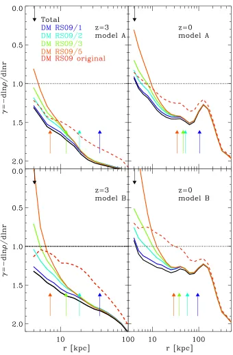
of Ruszkowski & Springel (2009). At z = 3 the dominant progenitor halos were populated with spherical model galaxies with and without accounting for adiabatic contraction. We apply a weighting scheme which allows us to change the relative amount of dark and stellar material assigned to each simulation particle in order to produce luminous properties which agree better with abundance matching arguments and observed bulge sizes atz = 3. This permits the study of the effect of initial compactness on the evolution of the mass-size relation. We find that for more compact initial stellar distributions the size of the final Brightest Cluster Galaxy grows with mass according tor _∝M2_{, whereas for more extended}

initial distributions, r_∝ M. Our results show that collisionless mergers in a cosmological context can reduce the strength of inner dark matter cusps with changes in logarithmic slope of 0.3 to 0.5 at fixed radius. Shallow cusps such as those found recently in several strong lensing clusters thus do not necessarily conflict with CDM, but may rather reflect on the initial structure of the progenitor galaxies, which was shaped at high redshift by their formation process.

4.2 Introduction

(50)

34 4. Shallow Dark Matter Cusps in Galaxy Clusters

and larger sizes respectively. Early theoretical studies investigated the role of cooling flows (Fabian, 1994) in BCG formation. This hypothesis is disfavoured by observations with Chandra and XMM-Newton which show that such flows are much weaker than required, as are the star formation rates in the central galaxies of clusters (McNamara et al., 2000; Fabian et al., 2001). Another scenario has BCGs growing by feeding on smaller galaxies (minor mergers). This is the notion of galactic cannibalism (Ostriker & Hausman, 1977; Hausman & Ostriker, 1978).

In the ΛCDM scenario, structures build-up hierarchically through accretion and merg-ers of smaller progenitors. Groups form before clustmerg-ers and have sufficiently low relative velocities that galaxy-galaxy mergers can occur before cluster formation, thus enhancing the formation of a massive central galaxy. De Lucia & Blaizot (2007) use semi-analytic galaxy formation models to show that in the ΛCDM cosmology, BCGs form primarily through in-situ star-formation at high redshifts, z _≥3, with subsequent mass growth dom-inated by non-dissipational merging. Similar processes are seen in hydrodynamical cos-mological simulations of massive galaxy formation (Naab et al., 2009; Oser et al., 2012a; Feldmann et al., 2011) although these are typically less effective at suppressing star for-mation at late times than semi-analytic models, leading to galaxies which are “younger” than those observed.

From this, it seems that many aspects of the late assembly of BCGs can be modelled without considering the early star formation phase. Dubinski (1998) was an early example of such work based on numerical N-body simulations of collisionless mergers of galaxies in a cosmological context. Dubinski found that the properties of cluster BCGs can be naturally explained by merging of galaxies which have already formed their stars at high redshift. This idea was further investigated by Ruszkowski & Springel (2009) (RS09) who studied the deviations of BCGs from the Kormendy and FJ relations in a ΛCDM simulation.

In relaxed clusters, BCGs reside at the bottom of the potential well, making them ideal probes of the distribution of dark matter from kpc to Mpc scales. Sand et al. (2002, 2004, 2008) studied a selection of clusters combining stellar dynamical modelling and strong gravitational lensing in order to infer the inner slope of the dark matter density profiles. Their studies found values for the logarithmic slope of the dark matter density profile

γ = ₋dln(ρ)/dlnr < 1, at odds with the predictions of dark-matter-only simulations of halo formation which generally follow the NFW profile with γNFW = 1 (Navarro et al.,

1997). More recently, Newman et al. (2011) revisited the study of Abell 383 by Sand et al. (2008), combining stellar kinematics, strong and weak lensing and X-ray data to deduce an inner slope of γ = 0.59+0−0..3035 at 95 percent confidence. These authors suggest this may

indicate a genuine problem with our understanding either of baryonic evolution or of the nature of the dark matter.

(51)

4.3 Numerical Methods 35

the scale of the central galaxy of a small group. However, the final masses of the central galaxies in these simulations are in general a factor of two or three higher than expected from abundance matching arguments (Guo et al., 2010; Moster et al., 2010; Behroozi et al., 2010), implying the need for a signicantly improved treatment of baryonic astrophysics. El-Zant et al. (2004) claimed that shallower cusps could be produced in a cluster through dynamical heating by the galaxies. However, they treated galaxies as unstrippable point masses which is too unrealistic to address the issue in quantitative detail.

At this stage it still seems interesting to address the second question by Newman et al. (2011): is the presence of shallow dark matter cusps at the centre of clusters a signifi-cant challenge to CDM? We use the RS09 simulation to test whether such cusps can be created through dry (i.e., gas-free) mergers. Recent observations of massive ellipticals at

z = 2 have shown that they were more compact than similar mass galaxies today (see e.g. van Dokkum et al., 2008). Dry, predominantly minor mergers have also been pro-posed as a possible mechanism to drive the required size evolution (e.g., Naab et al., 2009; Bezanson et al., 2009)

In this context a significant limitation of the RS09 simulations was that the galaxies they inserted at z = 3 had stellar masses an order of magnitude larger than expected from abundance matching arguments (Moster et al., 2010) and were assumed to follow the present-day mass-size relation. Here we remedy the inconsistencies between the simulations and observations by using a method that re-assigns the mixture of stellar and dark matter in each simulation particle. This enables us to study the evolution of stellar and dark matter distributions for different levels of initial compactness and stellar mass.

In Section 2, we give a description of the simulations as well as of the weighting scheme used in this study. We also present results on the mass and size growth of the BCG for different initial assignments of stars and dark matter. In Section 3, we look at how the initial slope of the dark matter evolves from z = 3 to the present. We discuss our results and conclude in Section 4.

4.3 Numerical Methods

4.3.1 Simulation

The simulations used for this study are described in detail in Ruszkowski & Springel (2009), (RS09) and we give only a short summary here. A cluster mass dark matter halo of 1015_M

⊙

was identified in the Millennium Simulation (Springel et al., 2005). The cosmological pa-rameters of this simulation are Ωm = 0.25, ΩΛ = 0.75, a scale-invariant slope of the power

spectrum of primordial fluctuations (n = 1.0), a fluctuation normalizationσ8 = 0.9, and a

Hubble constant H0 = 100hkm s−1Mpc−1 = 73 km s−1Mpc−1.

The cluster was then re-simulated using a zooming technique with a mass resolution of m = 1.57_×107_h−1_M

(52)

(1990) profile embedded in a NFW dark matter halo (Navarro et al., 1997). The masses of the dark matter and star particles were set to be identicalmdm=m∗ = 1.57× 107h−1M⊙

and they were assigned a softening length of ǫ = 1h−1_{kpc. comoving, half that of the}

other dark matter particles from the original resimulation. Throughout this paper we use

h= 0.73 and our mass and length units are thus in kpc and M⊙.

Two simulations were run with different initial galaxy models: one in which the dark matter was adiabatically contracted following Blumenthal et al. (1986) and one where it retained an undisturbed NFW profile. We shall refer to these as models A and B respec-tively. The Blumenthal et al. (1986) formalism over-predicts the amount of contraction observed in many hydrodynamical simulations (Gnedin et al., 2004), however through the inclusion of uncompressed and compressed dark halo models, we can probe two alternative regimes. If dry-merging is indeed the main driver in the late assembly of BCGs and if the RS09 initial galaxies were realistic, then the “real” solution would lie between these two models.

In fact, however, the galaxies which RS09 inserted at redshiftz = 3 followed the present-day mass-size relation from Shen et al. (2003) and assumed a stellar to dark matter mass ratio m∗/M = 0.1. This value is too large by a factor of 10 according to recent results from matching the observed high-redshift abundance of massive galaxies (Moster et al., 2010; Behroozi et al., 2010; Wake et al., 2011). We note that many other simulations in-vestigating similar processes have like-wise assumed over-massive stellar components (e.g., Nipoti et al., 2009; Rudick et al., 2011). However, we point out that for a given mass res-olution, more massive stellar bulges are represented by a larger number of particles which considerably improves the numerical convergence of the simulations.

Not surprisingly, the final merger remnants in RS09 were also too massivem∗ _∼1013_M

⊙

with half-mass radii which were too large (_∼ 100 kpc) compared to real BCGs. These generally do not exceed re ∼50kpc (Bernardi et al., 2007).

In order to study more consistently the change in the slope of dark matter density profiles at the centre of ΛCDM clusters, we need to address the question with galaxies that have stellar properties consistent with observations. We also need to test whether the final stellar mass of the merger remnant agrees with the stellar to halo mass relation (SHM) at z = 0 (Guo et al., 2010; Moster et al., 2010; Behroozi et al., 2010). We employ a weighting procedure to re-assign the luminous component of every initial galaxy such that only one percent of its total dark matter mass is locked in stars. For the range of halo masses (1013_M

⊙−1012M⊙) that we populate, abundance matching implies that this ratio

is rather constant. Additionally, our weighting scheme enables us to change the sizes of the luminous components to study the assembly of the BCG for different levels of compactness while keeping the total initial stellar mass fixed. We present this scheme in the next section.

4.3.2 Weighting Scheme

(53)

Figure 4.1: Differential energy distribution for the proto-BCG for the total mass and light contributions for three test cases re = reRS09/1, reRS09/2, reRS09/3, reRS09/5. Although

the reRS09/5 histogram intersects the total differential energy distribution, the particles in

(54)

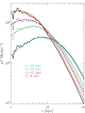
Figure 4.2: ρr2 _{profiles vs. radius for the four different realisations. The target functional}

(55)

to spherically symmetric density distributions. A galaxy is represented by a distribution of N particles of mass Mtot/N = mp and phase-space coordinates (x,v) which generate

the potential Φ = Φdark+ Φstellar= ΦNFW+ ΦHernquist. Each particle of energyE = 1₂v2+ Φ

now simultaneously represents dark matter and stars in different amounts according to a weight function ω(E) = f∗(E)/f(E). This is the ratio between the stellar distribution function (df_{) and the total} df_{. One can construct the stellar} df _{in the following way.}

In computing f∗(E), one assigns the particles a spherical number density distribution

ν(r) and solves the Eddington inversion formula:

f∗(_E) = √1 8π2

Z E

0

dΨ √

E −Ψ

d2_ν_(Ψ)

dΨ2 +

1 √ E dν dΨ Ψ=0 , (4.1)

where Ψ = ₋Φ + Φ0 and E = −E + Φ0 = Ψ−v2/2 are the relative potential and total

energies respectively. The potential used to generate the model galaxies in RS09 was a linear combination of a Hernquist and an NFW potential, both of which tend to zero in the limit r goes to infinity thus Φ0 = 0. We choose ν(r) to follow a Hernquist profile (1990):

ν(r) = a

r(r+a)3. (4.2)

The total df _{is the ratio of the differential energy distribution} _N₍_E_{) =} _dM/dE ₌

f(E)g(E) and the density of states g(E) which is solely defined by the potential Φ:

g(E) = (4π)2

Z rE

0

r2p2(E₋Φ(r))dr. (4.3)

Since Φ(r) andN(E) can both be measured directly from the simulation’s initial condition, this determines f(E).

Note that the only free parameter we have introduced is the scale radiusa for the light distribution which is related to the half-light radius by a = re/(

√

2 + 1). Within certain limits we can vary the relative mixture of dark and luminous matter to represent, for example, less massive and more compact bulges. This has the advantage of allowing us to study aspects of the assembly of massive galaxies fromz = 3 toz = 0 without having to run additional CPU intensive simulations, simply by tracking the weights to the final merger remnant. This scheme allows multiple interpretations of a single simulation. However, for our purposes the stellar mass within each galaxy is kept fixed, its value being dictated by abundance matching arguments, so it is the stellar and dark matter distributions which vary with the total mass distribution held fixed. Note that this implies that the initial dark matter distributions in the adjusted galaxies are no longer those expected naturally in ΛCDM. Thus while we can address issues of how the mixing of the two components changes inner profile shapes and is affected by initial compactness, we cannot expect the final DM distributions to be realistic.

(56)

Overplotted are stellar differential energy distributions for four reinterpretations with dif-ferent galaxy sizes: the original effective radius used in RS09 and the same reduced by factors of two, three and five. To show more explicitly that our method works we present

ρr2 _{profiles in Figure 2. Note that changing the sizes of the stellar component for a fixed}

m∗/Mhalo ratio, implies substantial changes in the inner slope of the dark matter profile.

The reduction of the stellar mass by a factor of 10 from that assumed in RS09 also means that both the uncontracted and contracted models now have overly concentrated dark matter distributions in the centres of the galaxy subhalos, except at very small radii where the reduced radii can lead to an increase of stellar density relative to RS09.

The maximum extent to which we are able to rescale the stellar component is set by the total mass profile. This is saturated by the stars alone at the softening radius if the RS09 sizes are reduced by a factor of _∼5 (see Figure 1).

The initial and final light profile shapes in the RS09/1 interpretation will be the same as in the original simulation, as only the stellar masses of every galaxy are changed (the inner dark matter profiles will differ, however, since they now contain the additional mass which used to be assigned to stars). This also means that the galaxies no longer lie on the Shen et al. (2003) stellar mass-size relation. In order to put them back on it (within the scatter) we need to reduce the sizes by factors of_∼5.

Recent observations show, however, that z = 2 elliptical galaxies were more compact than implied by the local relation (van Dokkum et al., 2008). Unfortunately, our spatial resolution limit does not permit us to consider such small sizes. We stress that these ob-servations still need to be treated with caution as the galaxy stellar masses are estimated photometrically. Martinez-Manso et al. (2011) argue that dynamical masses of compact galaxies at redshift z = 1 may be six times lower than some photometric estimates. Nev-ertheless if the photometrically determined stellar masses of galaxies at redshift z = 2 are even approximately correct, the galaxies should be even smaller than we assume in this paper. As we will see, the exercise presented here can nonetheless give insight into the puffing-up of BCGs by minor mergers and its dependance on the initial compactness of the galaxies.

4.3.3 Results for the BCG evolution

Size growth of the BCG

Fixing the stellar masses within all haloes according to abundance matching arguments (and hence reducing them by an order of magnitude from those originally assumed by RS09), we studied four assumptions for the compactness of the galaxies re = reRS09/1,

reRS09/2, reRS09/3, reRS09/5 in each of our two simulations. The trends arevery similar in

Laporte, Chervin F. P. (2014): Evolution of clusters and large-scale structures of galaxies. Dissertation, LMU München: Fakultät für Physik

Evolution of clusters and large-scale

structures of galaxies

Chervin F. P. Laporte

Evolution of clusters and large-scale

structures of galaxies

Chervin F. P. Laporte

Dissertation

an der Fakult¨

at f¨

ur Physik

der Ludwig–Maximilians–Universit¨

at

M¨

unchen

vorgelegt von

Chervin F. P. Laporte

aus Versailles, Yvelines, France

Contents

I

Overview

1

II

Brightest Cluster Galaxies and the distribution of dark matter in galaxy

31

List of Figures

List of Tables

Zusammenfassung

Summary

Part I

Chapter 1

Background Cosmology & Structure

Formation

1.1

Background Friedman Robertson-Walker

Cosmol-ogy

1.1.1

Inflation

1.2

A word on thermal history of the Universe

1.3

Growth of Structure in the linear regime and the

large-scale structures

1.3.1

Collisional fluid

1.4

Growth of matter and dark matter perturbations

after recombination

1.4.1

Primordial Power spectrum and its relation to the

Post-recombination one

Chapter 2

Dark Matter

2.1

Observational evidence

2.1.1

Galactic scales

2.1.2

Galaxy Cluster scales

2.1.3

Cosmological scales

2.1.4

Collisionless Cold Dark matter

2.2

Dark matter as a particle

2.2.1

WIMPs

2.2.2

axions

Chapter 3

Collisionless systems and the N-body

method

3.1

Dynamics of collisionless systems

3.2

N-body method

3.3

Force calculation and algorithms

3.3.1

Particle mesh method