Nonparametric estimation of mean residual life function using scale mixtures

Nonparametric Estimation of Mean Residual Life Function

Using Scale Mixtures

Shufang Liu

PRA International, Charlottesville, VA

Sujit K. Ghosh∗

Department of Statistics, North Carolina State University, Raleigh, NC 27695 ∗_{email: [email protected]}

Institute of Statistical Mimeo Series # 2612

Abstract

The mean residual life function (mrlf) of a subject is defined as the average residual lifetime of the subject given that the subject has survived up to a given time point. A smooth nonparametric estimator of the mrlf is proposed using a scale mixtures of the empirical estimate of the mrlf. Asymptotic properties are established. The performances of the proposed estimator are studied based on simulated data sets and finally, a real data set is used to illustrate the practical relevance of the proposed estimator.

Keywords: Mean residual life function; Right-censored data; Scale mixtures; Smooth nonparametric estimate.

1

Introduction

The mean residual life function, the hazard function, and the survival function are complementary in understanding aging process, since each of them can be obtained from any one of the other two functions. The mean residual life function can serve as a more useful tool than the survival function and the hazard function to assess the remaining life expectancy. The mean residual life function (mrlf ) of a lifetime random variable T with a finite expectation is defined as

m(t)≡E[T −t|T > t] =

∞

t S(u)

S(t)du, S(t)>0,

0 , otherwise, (1)

form can be specified. Tsang and Jardine (1993), Agarwal and Kalla (1996), Kalla et al. (2001), Gupta and Bradley (2003), Lai et al. (2004), and Gupta and Lvin (2005) utilized parametric approaches to estimate the mrlf. However, an incorrect specification of parametric assumptions is undesirable, especially when prediction is of interest. Many researchers then focus on using nonparametric estimation procedures to study m(t).

Yang (1978) employed the empirical survival function ˆS(t) in (1) to obtain the empirical estimate of m(t) for complete data. Ghorai et al. (1982) first used the estimator of Kaplan and Meier (1958) of S(t) into (1) to obtain the empirical estimate of m(t) for censored data. Since the empirical estimators of Yang and Ghorai et al. are discontinuous at each observation, smooth estimation of the mrlf has been developed. Essentially, all the methods derive the smooth versions of

m(t) by smoothing the survival functions. The kernel density method is often used. Kulasekara (1991) used the classical kernel density method. Ruiz and Guillamon (1996) used the recursive kernel density method. Abdous and Berred (2005) used the classical kernel density method with local linear fitting technique. Chaubey and Sen (1999) used the so called Hille’s theorem (Hille, 1948) to smooth the survival function only for complete data, which is given by

˜

m_n(t) = 1

λ_n

_n

k=0

_k

r=0((tλn)(k−r)/(k−r)!)Sn(k/λn)

(k=0)((tλn)k/k!)Sn(k/λn)

. (2)

In the simulation study, we extend the method of Chaubey and Sen (1999) to right-censored data. In this study, we propose scale mixtures to smooth ˆm_e(t) directly instead of first obtaining a smooth estimate of ˆS(t) in Section 2. In Section 3, we present a simulation study to evaluate the performance of the proposed mrlf, the empirical mrlf, and the smooth mrlf (Chauby and Sen, 1999). In Section 4, we compare the performance of the three mrlf estimators based on a real data set. In Section 5, we present some discussion and directions for further extensions.

2

A Scale Mixtures of the mrlf

Let T_i denote the survival time of the i-th subject for i= 1,2, . . . , n subjects. We denote the complete data set as D0 ={T_i : i= 1,2, . . . , n}. In many applications

given byD1 ={(X_i,Δ_i) :i= 1,2, . . . , n}. We assume that (T_i, C_i) are independent and identically distributed (iid) and further we assume that T is independent of

C.

In this section, we first introduce the Fellar Approximation Lemma and the Scale Mixture Theory. We then develop a smooth estimator ˆm_m(t) of m(t) us-ing the Feller Approximation Lemma. ˆm_m(t) happens to be a scale mixtures of the empirical mrlf ˆm_e(t). In the sense of the Scale Mixture Theory, ˆm_m(t) is a proper mrlf which satisfies the Characterization Thereom (Hall and Weller, 1981). We then present closed calculation forms for ˆm_e(t) and ˆm_m(t) for complete and censored data. Finally, we provide the asymptotic properties of ˆm_m(·).

First, we restate the result due to Petrone and Veronese (2002) based on Feller (1966, p.219).

Lemma 1. Feller Approximation Lemma:

Let g(·) be a bounded and right continuous function on R for each t. Let Z_k(t) be a sequence of random variables for each t such that μ_k(t) ≡ E[Z_k(t)] → t and

σ_k2(t)≡V ar[Z_k(t)]→0 as k → ∞. Then

E[g(Z_k(t))]→ g(t) ∀t.

The proof of the lemma is given in Appendix A. Now, we introduce the Scale Mixture Theory.

Theorem 1. Scale Mixture Theory: Let m(t) =E[T −t|T > t] be an mrlf. Then

(a) m(_θtθ)is a proper mrlf for any θ >0; (b) ₀+∞m(tθ)

θ π(θ)dθ is a proper mrlf for any density π(·) for [0,∞).

The proof of the theory is given in Appendix B. Now we propose a scale mix-tures of the empirical mrlf ˆm_e(t). It is known that ˆm_e(t) is a right continuous function on [0, T_(n)] and ˆm_e(t) = 0 fort > T_(n) and hence ˆm_e(t) is a bounded func-tion. Then, we can use the Feller Approximation Lemma to approximate ˆm_e(t) by ˆm_m(t). Let Z_n(t) ∼Ga(k_n, t

kn) for t >0, where Ga(kn,

t

kn) denotes a Gamma

distribution with meanμ_n(t) =t and varianceσ_n2(t) = _kt2

n and the density function

is given by

f_kn,t(z) =f

zk_n, t k_n

=

k_n t

kn ₁

Γ(k_n)z

Define,

ˆ

m_m(t) = E[ ˆm_e(Z_n(t))] = _∞

0

ˆ

m_e(u)dF_kn,t(u) (3)

= _∞

0

ˆ

m_e(tθ)

θ π(θ|kn)dθ, (4)

where π(θ|k_n) = kknn Γ(kn)θ

kn_e−knθ _{is the density function of a Ga(k}

n + 1,_k1_n)

distri-bution, and hence it follows from (b) of Theorem 1 that ˆm_m(t) is a scale mixture mrlf and it is a proper mrlf.

We give a unified closed calculation form for ˆm_e(t) for complete and censored data. Let the ordered observed data be 0 def= X₀ < X₁ < . . . < X_n < X_n+1 def= ∞. The empirical mrlf ˆm_e(t) can be expressed as

ˆ

m_e(t) =

n

j=1(Xj−t)I(Xj−t)wj

n

j=1I(Xj−t)wj , if 0< t≤Xn,

0 , if t > X_n, (5)

=

n

j=l+1Xjwj

n

j=l+1wj −t, if Xl ≤t < Xl+1, l= 0,1, . . . , n−1,

0 , if t > X_n, (6)

where w_j = F_n(X_j)− F_n(X_j−) and F_n(X_j) is the KM estimate. Notice that

w_j = 1/n for complete data.

Then, ˆm_m(t) can also be calculated with the same closed form for complete and censored data. The details of the calculation are given in the Appendix C.

ˆ mm(t) =

_∞

0

ˆ me(u)f

ukn, t

kn

du (7)

=

n−1

l=0

_n

j=l+1Xjwj

_n

j=l+1wj

F

Xl+1kn, t kn

−F

Xlkn, t kn

−tF

Xnkn+ 1, t kn

, (8)

where F(·|k_n, t

kn) is the cdf of Ga(kn,

t

kn).

Remark1. If F_n(X_j)is the cdf estimate for data with tied observations, mˆ_e(t) and mˆ_m(t) based on data with tied observations can be caluculated using the same closed forms as (6,8).

Next we show that ˆm_m(t) is a smooth mrlf. To be a smooth estimate ofm(t), ˆ

m_m(t) must satisfy the following conditions:

(i) π(θ|k_n) is a smooth density on [0,∞) such that ₀∞ 1

θπ(θ|kn)dθ < ∞ for all

(ii) If Y_n∼π_n(·|k_n) then Y_n→P 1 as n → ∞.

Since

∞

0

1

θπ(θ|kn)dθ =

_∞

0

1

θ kkn

n

Γ(k_n)θ

kn_e−knθ _{= 1,}

condition (i) is satisfied.

SinceY_n∼Ga(k_n+ 1,1/k_n),

E[Y_n] = kn+ 1

k_n = 1 +

1

k_n →1 as n→ ∞

and

var[Y_n] = kn+ 1

k_n2 =

k_n+ 1

k_n

1

k_n →0 as n → ∞,

then condition (ii) is satisfied. Therefore ˆm_m(t) is a smooth estimator.

Under conditions (i) and (ii) and the assumption of k_n = cn1+ where > 0 and c is a constant, we claim that ˆm_m(t) has the following properties:

Theorem 2. mˆ_m(t) pointwisely converges in probability to m(t).

Theorem 3. √n( ˆm_m(t) − m(t)) is asymptotically a Gaussian process with mean identically zero and covaraince function σ(s, t), where

σ(s, t) = 1

S(s)S(t) _∞

t

u2dF(u)− 1

S(t)

_∞

t

udF(u) ₂

, 0≤s≤t <∞

for complete data and

σ(s, t) = 1

S(s)S(t) _∞

t

φ2(ν)

(S(ν)G(ν))2dH(ν), 0≤s≤t <∞,

where φ(t) = ∞

t S(u)du, G(t) = P r[C > t], and H(t) = P r[Δ1 = 1, X1 ≤ t] for

censored data.

We know that ˆm_e(t) for complete data by Yang(1978) and ˆm_e(t) for right-censored by Ghorai et al. (1982) have the following asymptotic properties:

(a) ˆm_e(t) pointwisely converges in probability to m(t):

lim

n→∞P(|mˆe(t)−m(t)| ≥) = 0.

Now we prove Theorem 2.

Proof:

Since ˆm_e(t) pointwisely converges in probability to m(t) from Yang (1978) and Ghorai et al. (1982), i.e.,

ˆ

m_e(t)→P m(t) as n→ ∞

and

Y_n→P 1 as n → ∞,

then by Slutsky’s Theorem

ˆ

m_e(tY_n)

Y_n

P

→ m(t∗1)

1 =m(t).

Notice that mˆe_Y(tYn)

n is the mrlf of ˜

Tn

Yn, where ˜Tn takes T1, . . . , Tn with probability of 1

n each. Then we can see thatE[ ˜

Tn

Yn−t|

˜

Tn

Yn > t, Yn] is bounded. Thus we can obtain

the following relationship by DCT

E

ˆ

m_e(tY_n)

Y_n

P

→E[m(t)] wrtπ,

i.e.,

ˆ

m_m(t)→P m(t).

This completes the proof of Theorem 2.

Now we prove Theorem 3.

Proof:

√

n( ˆm_m(t)−m(t)) = √n( ˆm_m(t)−mˆ_e(t)) +√n( ˆm_e(t)−m(t)),

where √n( ˆm_e(t)−m(t))∼GP(0, σ(·,·)).

Now we consider √n( ˆm_m(t)−mˆ_e(t)) = √nE[mˆe(tYn)

Yn −mˆe(t)].

First, we take Taylor’s expansion on mˆe(tYn)

Yn

ˆ

m_e(tY_n)

Y_n =

ˆ

m_e(t)

Y_n +

(tY_n−t) ˆm_e(t∗_n)

Y_n ,

where t∗_n→P t asn → ∞. It can be seen from (6) that ˆm_e(t) is differentiable ifft ∈

Second, we substitute the Taylor’s expansion into√nE[mˆe(tYn)

Yn −mˆe(t)]

√

n( ˆm_m(t)−mˆ_e(t)) = √nE[mˆe(tYn)

Y_n −mˆe(t)]

= √nE

ˆ

m_e(t)

Y_n −mˆe(t) +

(tY_n−t) ˆm_e(t∗_n)

Y_n = E _√ n 1

Y_n −1

ˆ

m_e(t)−√n

1

Y_n −1

tmˆ_e(t∗_n)

If we can prove√n

1

Yn −1

P

→0 asn → ∞, then we can obtain√n( ˆm_m(t)−

ˆ

m_e(t))→P 0 as n → ∞and the proof is complete. SinceY_n∼Ga(k_n+ 1,1/k_n), then

E

_√

n

1

Y_n −1

=√n

E 1 Y_n −1 =√n

k_n

k_n+ 1−1 −1 = 0 and V ar _√ n 1

Y_n −1

=n∗V ar

1

Y_n

=n k

2 n

k2_n(k_n−1) =

n k_n−1.

Since we assumek_n =cn1+_{where >0, it can be seen thatvar}√_n1

Yn −1

→

0 as n→ ∞. Therefore, √n

1

Yn −1

P

→0 asn → ∞is proved. Hence, this com-pletes the proof of Theorem 3.

Remark 2. Notice that the asymptotic properties of mˆ_m(t) are the same as those of the estimator of Yang (1978) for complete data and the same as those of the estimator of Ghorai et al. (1982) for censored data.

3

A Simulation Study

• The data are generated from Wei(2, 2). The performance of emrlf, smrlf, and mmrlf is evaluated at the time points from quantile 0.01 to quantile 0.90 of this distribution.

• The censoring distribution is Exp(λ). The choices ofλto obtain the averaged censoring rates of 0%, 20%, 40%, and 60% are listed in the following table:

Censoring Rate Exp

0% λ=∞

20% λ= 7.633

40% λ= 3.225 60% λ= 1.667

• A sample size of n = 100 and a Monte Carlo sample size of N = 1000 are used.

• The parameter k_n in the Gamma distribution to calculate the scale mixture mrlf ˆm_m(t) (mmrlf) is set to be n1.01_.

• The bias can be estimated as ˆB(t) =

_N

i=1mˆi(t)

N −m(t), and then the relative

bias is B_mˆ(₍t_t)₎. The MSE can be estimated as M SE(t) = _N1₋₁N_i=1( ˆm_i(t)− ¯

ˆ

m(t))2 + ( ¯mˆ(t)−m(t))2. The relative efficiency M SEemrlf(t)

M SEmmrlf(t) and

M SEemrlf(t)

M SEsmrlf(t)

is compared.

Figures 1-4 show the graphical summary of the simulation for the targeted censoring rates of 0%, 20%, 40%, and 60%, respectively. In each figure, Panels 1, 3, and 5 feature the boxplots of the 1000 replications of ˆm(t) changing with time for emrlf, mmrlf, and smrlf, respectively. Panel 2 compares the averaged emrlf, mmrlf, and smrlf from the 1000 replications with the true mrlf. Panel 4 compares the bias of averaged emrlf, mmrlf, and smrlf with 0. Panel 6 shows the relative efficiency (RE) of emrlf to mmrlf (in dotted line), emrlf to smrlf (in dash line). Tables 2-5 list the relative bias and the relative efficiency for the experiments of the censoring rates of 0%, 20%, 40%, and 60%, respectively.

mmrlf, and smrlf increases with the censoring rate as expected. With the increase of the censoring rate, the bias for emrlf, mmrlf, and smrlf also increase. These are reasonable results, because the information provided by the data is limited by the censored observations.

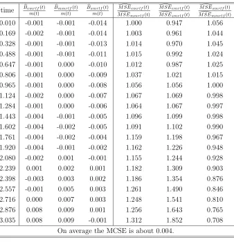
Figure 1 and Table 2 present the simulation results for data with 0% censoring rate, i.e., complete data. It can be seen from Figure 1 that emrlf, mmrlf, and smrlf have the similar performance for the small and moderate time points. While emrlf has the largest variation and the smrlf has the least variation for the extreme time points. From Table 2, it can be seen that smrlf has larger relative biases at small time points compared to emrlf and mmrlf. It turns out that these biases of smrlf are statistically significant (P-value < 0.05) for all time points smaller than 1.92 (the 33%tile of this Weibull distribution). Generally, mmrlf has smaller biases than emrlf, though none of the biases from emrlf or mmrlf are significantly different from 0. In terms of relative efficiency, mmrlf is always better than emrlf. The smrlf is less efficient for small time points and more efficient for large time points compared to emrlf and smrlf. Therefore, based on relative bias and relative efficiency, mmrlf is a better estimator compared to emrlf, and mmrlf is a better estimator for small time points compared to smrlf. The reason why smrlf does better for large time points might be that the number of the observations used to calculate mmrlf and emrlf decreases with the increase of time, while the number of the observation used to calculate smrlf stays the same. In summary, mmrlf is a definitely better estimator compared to emrlf and a competitive estimator to smrlf for complete data.

Figure 2 and Table 3 present the simulation results for data with 20% censoring rate. We get the similar results for slightly censored data as for the complete data, i.e., mmrlf is a better estimator compared to emrlf and a better estimator for small data points compared to smrlf.

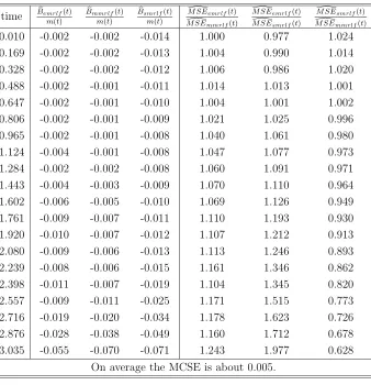
Figure 3 and Table 4 present the simulation results for data with 40% censoring rate. For all the time points studied in this simulation, smrlf is significantly biased. It appears that emrlf and mmrlf are only biased for time points larger than quantile 0.875 (P-value <0.05). Therefore, for moderately censored data, mmrlf is better than emrlf and smrlf.

and smrlf are smaller than those from smrlf. Therefore, for highly censored data, emrlf, smrlf and mmrlf are not so good estimators.

Considering the fact that we sometimes may encounter data sets with a very large sample size, we attempted to compare the performance of emrlf, mmrlf, and smrlf for a simulation study for data with a sample size of 5000. We set the other conditions as before, except that the sample size n changed to 5000 from 100. Since the calculation of smrlf involves smoothing the survival function in the numerator and denominator (see (2)), the computation for data with a sample size of 5000 is very intensive. We failed to do the simulation for smrlf under our computing resource. Since ˆm_e(t) and ˆm_m(t) have closed calculation forms, it did not take much time to do the simulation for emrlf and mmrlf. The results show that mmrlf is more efficient compared to emrlf for data with a very large sample size.

4

Application to a Melanoma Study

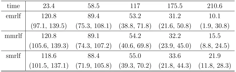
We apply our estimation methods to the data set given in Ghorai et al. (1982). This data set has the survival times (in weeks) of 68 participants of a melanoma study conducted by the Central Oncology Group with headquarters at the Univer-sity of Wisconsin-Madison. This data set has a censoring rate of 58.8%.

Figure 5 shows the results of the three methods. Panel 1 compares emrlf, mmrlf, and smrlf. Panel 2-4 show the 95% asymptotic confidence interval from case resampling for emrlf, mmrlf, and smrlf, respectively. It can be seen that emrlf, mmrlf, and smrlf have similar results for this highly censored data. However, unlike emrlf is a discontinuous estimator, mmrlf and smrlf are smooth estimators. It also can be seen that emrlf vanishes at the largest time point, while mmrlf and smrlf can take positive values. This indicates that mmrlf and smrlf can have a better prediction performance than emrlf even outside the observed time range.

Table 1: Estimated mrlf’s with 95% CI at some time points for the Melanoma study

time 23.4 58.5 117 175.5 210.6

emrlf 120.8 89.4 53.2 31.2 10.1

(97.1, 139.5) (75.3, 108.1) (38.8, 71.8) (21.6, 50.8) (1.9, 30.8)

mmrlf 120.8 89.1 54.2 32.2 15.5

(105.6, 139.3) (74.3, 107.2) (40.6, 69.8) (23.9, 45.0) (8.8, 24.5)

smrlf 118.6 88.4 55.0 33.6 21.9

(101.5, 137.1) (71.9, 105.8) (39.3, 70.2) (21.8, 44.3) (11.8, 28.3)

given that the patient has already survived at least 117 weeks after entering the study. Also a 95% confidence interval for ˆm_m(117) is (40.6, 69.8), which indicates that it is highly unlikely that the patient will survival beyond about 70 weeks and it is also highly unlikely that the patient will survival less than about 40 weeks after entering the study for 117 weeks.

Notice that the conclusions derived from Table 1 can not be made using the hazard function directly. This illustrates one of the advantages of using the mean residual life function over the traditional hazard function.

5

Discussion

In the literature, researchers often first estimate the survival function and then calculate ˆm_e(t). The closed form of ˆm_e(t) from (6) provides an easy and unified calculation procedure for complete data and right-censored data. The closed form of our scale mixture mrlf ˆm_m(t) from (8) is a nonparametric smooth estimator of the mrlf for complete and right censored data.

ˆ

m_m(t) is always a better estimator compared to ˆm_e(t). In terms of bias, ˆm_m(t) is always a better estimator compared to the Chaubey and Sen’s (1999) estimator

ˆ

m_s(t). In terms of MSE, ˆm_m(t) is competitive to ˆm_s(t).

Finally, ˆm_e(t) and ˆm_m(t) are computationally less demanding compared to the ˆ

0.01 0.68 1.35 2.03 2.7

0123

emrlf

0.0 0.5 1.0 1.5 2.0 2.5 3.0

0.6

1.0

1.4

1.8

averaged mrlf

0.01 0.68 1.35 2.03 2.7

0123

mmrlf

0.0 0.5 1.0 1.5 2.0 2.5 3.0

−0.03

−0.01

0.01

bias emrlf

mmrlf smrlf

0.01 0.68 1.35 2.03 2.7

0123

time points

smrlf

0.0 0.5 1.0 1.5 2.0 2.5 3.0

0.8

1.2

1.6

2.0

time points

RE

emrlf/mmrlf emrlf/smrlf

Figure 1: Estimated emrlf, mmrlf, and smrlf under 0% censoring rate

0.01 0.68 1.35 2.03 2.7

0123

emrlf

0.0 0.5 1.0 1.5 2.0 2.5 3.0

0.6

1.0

1.4

1.8

averaged mrlf

0.01 0.68 1.35 2.03 2.7

0123

mmrlf

0.0 0.5 1.0 1.5 2.0 2.5 3.0

−0.03

−0.01

0.01

bias emrlf

mmrlf smrlf

0.01 0.68 1.35 2.03 2.7

0123

time points

smrlf

0.0 0.5 1.0 1.5 2.0 2.5 3.0

0.8

1.2

1.6

2.0

time points

RE

emrlf/mmrlf emrlf/smrlf

0.01 0.68 1.35 2.03 2.7

0123

emrlf

0.0 0.5 1.0 1.5 2.0 2.5 3.0

0.6

1.0

1.4

1.8

averaged mrlf

0.01 0.68 1.35 2.03 2.7

0123

mmrlf

0.0 0.5 1.0 1.5 2.0 2.5 3.0

−0.03

−0.01

0.01

bias

emrlf mmrlf smrlf

0.01 0.68 1.35 2.03 2.7

0123

time points

smrlf

0.0 0.5 1.0 1.5 2.0 2.5 3.0

0.8

1.2

1.6

2.0

time points

RE

emrlf/mmrlf emrlf/smrlf

Figure 3: Estimated emrlf, mmrlf, and smrlf under 40% censoring rate

0.01 0.68 1.35 2.03 2.7

0123

emrlf

0.0 0.5 1.0 1.5 2.0 2.5 3.0

0.6

1.0

1.4

1.8

averaged mrlf

0.01 0.68 1.35 2.03 2.7

0123

mmrlf

0.0 0.5 1.0 1.5 2.0 2.5 3.0

−0.20

−0.10

0.00

bias emrlf

mmrlf smrlf

0.01 0.68 1.35 2.03 2.7

0123

time points

smrlf

0.0 0.5 1.0 1.5 2.0 2.5 3.0

0.8

1.2

1.6

2.0

time points

RE

emrlf/mmrlf emrlf/smrlf

Table 2: Relative biases and efficiency of estimated mrlf’s under 0% censoring rate

time Bemrlf(t) m(t)

Bmmrlf(t) m(t)

Bsmrlf(t) m(t)

M SEemrlf(t)

M SEmmrlf(t)

M SEemrlf(t)

M SEsmrlf(t)

M SEsmrlf(t)

M SEmmrlf(t)

0.010 -0.001 -0.001 -0.014 1.000 0.947 1.056 0.169 -0.002 -0.001 -0.014 1.003 0.961 1.044 0.328 -0.001 -0.001 -0.013 1.014 0.970 1.045 0.488 -0.001 -0.001 -0.011 1.015 0.992 1.024 0.647 -0.001 0.000 -0.010 1.012 0.987 1.025 0.806 -0.001 0.000 -0.009 1.037 1.021 1.015 0.965 -0.001 0.000 -0.008 1.056 1.056 1.000 1.124 -0.002 0.000 -0.007 1.067 1.069 0.998 1.284 -0.001 0.000 -0.006 1.064 1.067 0.997 1.443 -0.004 -0.001 -0.005 1.096 1.099 0.998 1.602 -0.004 -0.002 -0.005 1.091 1.102 0.990 1.761 -0.004 -0.002 -0.004 1.159 1.198 0.967 1.920 -0.004 -0.001 -0.002 1.162 1.226 0.948 2.080 -0.002 0.001 -0.001 1.155 1.244 0.928 2.239 0.001 0.002 0.001 1.182 1.309 0.903 2.398 -0.003 0.003 0.002 1.186 1.354 0.876 2.557 -0.001 0.005 0.003 1.261 1.490 0.846 2.716 0.000 0.007 0.003 1.248 1.541 0.810 2.876 0.008 0.009 0.001 1.256 1.643 0.765 3.035 0.008 0.009 -0.001 1.312 1.852 0.708

On average the MCSE is about 0.004.

Table 3: Relative biases and efficiency of estimated mrlf’s under 20% censoring rate

time Bemrlf(t) m(t)

Bmmrlf(t) m(t)

Bsmrlf(t) m(t)

M SEemrlf(t)

M SEmmrlf(t)

M SEemrlf(t)

M SEsmrlf(t)

M SEsmrlf(t)

M SEmmrlf(t)

0.010 -0.001 -0.001 -0.013 1.000 0.966 1.036 0.169 -0.001 -0.001 -0.013 1.002 0.977 1.026 0.328 -0.001 -0.001 -0.012 1.010 0.981 1.030 0.488 0.000 0.000 -0.010 1.013 1.007 1.006 0.647 0.000 0.001 -0.009 1.010 1.002 1.008 0.806 0.000 0.001 -0.007 1.035 1.038 0.998 0.965 0.000 0.001 -0.006 1.052 1.067 0.986 1.124 -0.001 0.001 -0.005 1.057 1.077 0.981 1.284 0.001 0.001 -0.005 1.063 1.084 0.981 1.443 -0.001 0.001 -0.004 1.083 1.105 0.980 1.602 -0.002 -0.001 -0.004 1.083 1.117 0.969 1.761 -0.005 -0.002 -0.004 1.124 1.187 0.947 1.920 -0.005 -0.002 -0.004 1.152 1.240 0.929 2.080 -0.005 -0.001 -0.004 1.143 1.253 0.912 2.239 -0.002 0.000 -0.004 1.160 1.308 0.887 2.398 -0.006 0.000 -0.004 1.177 1.374 0.857 2.557 -0.002 0.002 -0.005 1.222 1.486 0.822 2.716 -0.005 0.003 -0.008 1.178 1.517 0.777 2.876 0.002 0.003 -0.012 1.237 1.722 0.718 3.035 0.000 -0.002 -0.018 1.292 1.963 0.658

Table 4: Relative biases and efficiency of estimated mrlf’s under 40% censoring rate

time Bemrlf(t) m(t)

Bmmrlf(t) m(t)

Bsmrlf(t) m(t)

M SEemrlf(t)

M SEmmrlf(t)

M SEemrlf(t)

M SEsmrlf(t)

M SEsmrlf(t)

M SEmmrlf(t)

0.010 -0.002 -0.002 -0.014 1.000 0.977 1.024 0.169 -0.002 -0.002 -0.013 1.004 0.990 1.014 0.328 -0.002 -0.002 -0.012 1.006 0.986 1.020 0.488 -0.002 -0.001 -0.011 1.014 1.013 1.001 0.647 -0.002 -0.001 -0.010 1.004 1.001 1.002 0.806 -0.002 -0.001 -0.009 1.021 1.025 0.996 0.965 -0.002 -0.001 -0.008 1.040 1.061 0.980 1.124 -0.004 -0.001 -0.008 1.047 1.077 0.973 1.284 -0.002 -0.002 -0.008 1.060 1.091 0.971 1.443 -0.004 -0.003 -0.009 1.070 1.110 0.964 1.602 -0.006 -0.005 -0.010 1.069 1.126 0.949 1.761 -0.009 -0.007 -0.011 1.110 1.193 0.930 1.920 -0.010 -0.007 -0.012 1.107 1.212 0.913 2.080 -0.009 -0.006 -0.013 1.113 1.246 0.893 2.239 -0.008 -0.006 -0.015 1.161 1.346 0.862 2.398 -0.011 -0.007 -0.019 1.104 1.345 0.820 2.557 -0.009 -0.011 -0.025 1.171 1.515 0.773 2.716 -0.019 -0.020 -0.034 1.178 1.623 0.726 2.876 -0.028 -0.038 -0.049 1.160 1.712 0.678 3.035 -0.055 -0.070 -0.071 1.243 1.977 0.628

On average the MCSE is about 0.005.

Table 5: Relative biases and efficiency of estimated mrlf’s under 60% censoring rate

time Bemrlf(t) m(t)

Bmmrlf(t) m(t)

Bsmrlf(t) m(t)

M SEemrlf(t)

M SEmmrlf(t)

M SEemrlf(t)

M SEsmrlf(t)

M SEsmrlf(t)

M SEmmrlf(t)

0.010 -0.010 -0.010 -0.020 1.000 0.974 1.027 0.169 -0.010 -0.010 -0.021 1.003 0.980 1.023 0.328 -0.011 -0.011 -0.021 1.007 0.986 1.022 0.488 -0.011 -0.011 -0.020 1.010 0.988 1.023 0.647 -0.013 -0.012 -0.021 1.005 0.987 1.018 0.806 -0.014 -0.013 -0.022 1.022 1.014 1.008 0.965 -0.017 -0.016 -0.024 1.020 1.026 0.994 1.124 -0.022 -0.019 -0.027 1.043 1.063 0.981 1.284 -0.023 -0.022 -0.030 1.046 1.073 0.975 1.443 -0.028 -0.026 -0.034 1.030 1.074 0.959 1.602 -0.033 -0.031 -0.039 1.092 1.174 0.930 1.761 -0.039 -0.037 -0.046 1.088 1.201 0.906 1.920 -0.047 -0.044 -0.054 1.095 1.242 0.882 2.080 -0.055 -0.052 -0.065 1.102 1.300 0.848 2.239 -0.058 -0.065 -0.081 1.114 1.394 0.799 2.398 -0.081 -0.087 -0.102 1.132 1.531 0.739 2.557 -0.110 -0.124 -0.131 1.162 1.711 0.680 2.716 -0.155 -0.176 -0.168 1.206 1.921 0.628 2.876 -0.233 -0.246 -0.213 1.196 2.066 0.579 3.035 -0.332 -0.329 -0.266 1.203 2.295 0.524

50 100 150 200

0

2

0

4

0

6

0

8

0

100

120

mrlf

emrlf mmrlf smrlf

50 100 150 200

0

2

0

4

0

6

0

8

0

100

120

emrlf

50 100 150 200

20

40

60

80

100

120

time points

mmrlf

50 100 150 200

20

40

60

80

100

120

time points

smrlf

References

Abdous, B. and Berred, A. (2005). Mean Residual Life Estimation. Journal of Statistical Planning and Inference 132, 3-19.

Agarwal, S.L. and Kalla, S.L. (1996). A Generalized Gamma Distribution and its Application in Reliability, Communications in Statistics, Theory and Meth-ods 25, 201-210.

Chaubey, Y.P. and Sen, P.K. (1999). On Smooth Estimation of Mean Residual Life. Journal of Statistical Planning and Inference 75, 223-236.

Feller W. (1966). An Introduction to Probability Theory and its Applications. Vol. II. Wiley, New York.

Ghorai, J., Susarla, A., Susarla, V., and Van-Ryzin, J. (1982). Nonparametric Estimation of Mean Residual Life Time with Censored Data. Nonparametric Statistical Inference. Vol.I, Colloquia Mathematica Societatis, 32. North-Holland, Amsterdam-New York, 269-291.

Gupta, R.C. and Bradley, D.M. (2003). Representing the Mean Residual Life in Terms of the Failure Rate. Mathematical and Computer Modelling 37, 1271-1280.

Gupta, R.C. and Lvin, S. (2005). Monotonicity of Failure Rate and Mean Resid-ual Life Function of a Gamma-type Model. Applied Mathematics and Com-putation 165, 623-633.

Hall, W.J. and Wellner, J.A. (1981). Mean Residual Life. Statistics and Related Topics. Edited by M. Csorgo, D.A. Dawson, J.N.K. Rao , and A.K.Md.E. Saleh. North-Holland, Amsterdam. 169-184.

Hille, E. (1948). Functional Analysis and Semigruops. Am.Math.Soc.Colloq. Pub., Vol.31, American Mathematical Society.

Kalla, S.L., Al-Saqabi, H.G., Khajah, H.G. (2001). A Unified Form of Gamma-type Distributions. Applied Mathematics and Computation 118, 175-187.

Kulasekera, K.B. (1991). Smooth Nonparametric Estimation of Mean Residual Life. Microelectron. Reliability 31(1), 97-108.

Lai, C.D., Zhang, L., Xie, M. (2004). Mean Residual Life and Other Properties of Weibull Related Bathtub Shape Failure Rate Distributions. International Journal of Reliability, Quality and Safety Engineering 11, 113-132.

Petrone, S. and Veronese, P. (2002). Non Parametric Mixture Priors Based on an Exponential Random Scheme. Statistical Methods and Applications 11, 105-116.

Ruiz, J.M. and Guillamon, A. (1996). Nonparametric Recursive Estimator of Residual Life and Vitality Funcitons under Mixing Dependence Condtions. Communcation in Statistics, Theory and Methods 4, 1999-2011.

Tsang, A.H.C. and Jardine, A.K.S. (1993). Estimation of 2-parameter Weibull Distribution from Incomplete Data with Residual Lifetimes. IEEE Thans. Reliablity 42, 291-298.

Appendix A

Proof of Feller Approximation Lemma:

Let F_k,t denote the cumulative distribution function of Z_k(t). Since g is right continuous at t, given > 0 there exists δ₁ > 0 such that z ∈ (t, t+ δ₁) ⇒

|g(z)−g(t)|< and P[t−δ₁ < Z_k(t)< t]< . Since g is bounded, we can find a

δ₀ such that |g| ≤M for all z−t ≥δ₀. Take δ=max(δ₁, δ₀), then

|E(g(Z_k(t)))−g(t)| ≤E[|g(Z_k(t))−g(t)|]

=

|g(z)−g(t)|dF_k,t(z)

=

z∈(t,t+δ)

|g(z)−g(t)|dF_k,t(z) +

z /∈(t,t+δ)

|g(z)−g(t)|dF_k,t(z)

≤ P[t < Z_k(t)< t+δ] + 2M P[Z_k(t)< t orZ_k(t)> t+δ]

≤ + 2M{P[|Z_k(t)−t|> δ] +P[t−δ₁ < Z_k(t)< t]}

≤ + 2M

σ_k2(t)

δ2 +

Let k→ ∞, we get σ_k2(t)→0 and

lim

k→∞E[|g(Zk(t))−g(t)|]≤.

But >0 is arbitrary, so

lim

k→∞E[|g(Zk(t))−g(t)|] = 0,

i.e.,

lim

k→∞E(g(Zk(t))) =g(t).

Appendix B

Proof of the Scale Mixture Theory:

Proof: Notice that, for θ >0,

m(tθ)

θ = E[T −tθ|T > tθ]

1

θ

= E

T θ −t

T θ > t

.

Hence m(_θtθ) is the mrlf of T_θ and (a) is proved. Next,

_∞

0

m(tθ)

θ π(θ)dθ = Eπ

E

T θ −t

T_θ > tθ

= E

T θ −t

T_θ > t

Hence, ₀∞ m(tθ)

θ π(θ)dθ is the mrlf of Tθ where Tθ|θ∼ m(tθ)

θ and θ∼ π(·), and (b) is

proved. Notice that the mrlf uniquely determines a distribution, thus T_θ|θ∼ m(_θtθ), which means that the conditional distribution of T

θ given θ is the distribution

Appendix C

The details of the calculation of mˆ_m(t):

ˆ

m_m(t), the smooth estimator of m(t) for censored data ( complete data are special case of censored data where weight functionw_j = 1

n), can be calulated with

a closed form. The details of the calculation are given here.

ˆ mm(t) =

_∞

0 mˆe(u)f

ukn, t kn du= n−1 l=0 _Xl+1 Xl ˆ me(u)f

ukn, t kn du = n−1 l=0 _n

j=l+1Xjwj

_n

j=l+1wj

_Xl+1

Xl

f

ukn, t

kn du− _Xl+1 Xl uf

ukn, t

kn du = n−1 l=0 ⎡ ⎢ ⎣ _n

j=l+1Xjwj

_n

j=l+1wj

_Xl+1

Xl

f

ukn, t kn du− _Xl+1 Xl uu

kn−1

t kn

kn

Γ(kn) e

−( t kn)u_du

⎤ ⎥ ⎦ = n−1 l=0 _n

j=l+1Xjwj

_n

j=l+1wj

_Xl+1

Xl

f

ukn, t

kn du− t kn _kn 1 Γ(kn)

_Xl+1

Xl

ukn_e−(knt )u_du

= n−1 l=0 ⎡ ⎢ ⎣ _n

j=l+1Xjwj

_n

j=l+1wj

_Xl+1

Xl

f

ukn, t

kn

du−Γ(kn+ 1) Γ(kn)

t kn

_Xl+1

Xl

ukn

t kn

kn+1

Γ(kn+ 1) e

−( t kn)u_du

⎤ ⎥ ⎦ = n−1 l=0 _n

j=l+1Xjwj

_n

j=l+1wj

_Xl+1

Xl

f

ukn, t kn

du−t

_Xl+1

Xl

f

ukn+ 1, t kn du = n−1 l=0 n

j=l+1Xjwj

_n

j=l+1wj

F

Xl+1

kn, t

kn −F Xl kn, t

kn − n−1 l=0 t F

Xl+1kn+ 1, t

kn

−F

Xlkn+ 1, t

kn = n−1 l=0 _n

j=l+1Xjwj

_n

j=l+1wj

F

Xl+1kn, t kn

−F

Xlkn, t kn −t F

Xnkn+ 1, t kn

−F

X0kn+ 1, t kn = n−1 l=0 _n

j=l+1Xjwj

_n

j=l+1wj

F

Xl+1kn, t kn

−F

Xlkn, t kn

−tF

Xnkn+ 1, t kn

,