ABSTRACT
DAY, JOSHUA THOMAS. Online Algorithms for Statistics. (Under the direction of Dr. Hua Zhou and Dr. Eric Laber.)
Traditional algorithms for calculating statistics and models are often infeasible when working with big data. A statistician will run into problems of not just scalability, but of handling data arriving in a continuous stream. Online algorithms, which update esti-mates one observation at a time, can naturally handle big and streaming data. Many traditional (offline) algorithms have online counterparts that produce exact estimates, but this is not always possible. There exists a variety of online (stochastic approxima-tion) algorithms for approximate solutions, but there is no universally “best” algorithm and convergence can be sensitive to the choice of learning rate, a decreasing se-quence of step sizes.
Majorization-minimization (MM) is an optimization concept that has not received much attention in the stochastic approximation (SA) literature. MM is an intuitive idea of iteratively solving easier problems that guarantee a decrease in the objective func-tion that incorporates some second-order informafunc-tion in each iterafunc-tion. The current state-of-the-art SA algorithms are based entirely on first-order (gradient) information and therefore ignore potentially useful information in each update. We derive two new algorithms for incorporating MM concepts into SA that have strong stability properties. The first algorithm (OMAP) is similar in spirit to the Stochastic MM Algorithm (Mairal, 2013b), referred to here as OMAS. We analyze OMAP and OMAS in a unified frame-work and offer stronger convergence results for OMAS than in the original paper. The second algorithm (MSPI) incorporates the MM concept into Implicit Stochastic Gradient Descent (Toulis and Airoldi, 2015) and Stochastic Proximal Iteration (Ryu and Boyd, 2014). Compared to the algorithms on which it is based, MSPI can solve a wider class of problems and in many cases has a cheaper online update. For all three MM-based algorithms, it is typically straightforward to translate existing offline MM algorithms into an online counterpart, particularly in the case of quadratic majorizations.
rithms typically focus on a small class of problems or specific type of algorithm. To our knowledge, OnlineStats is unique in the way algorithms are represented, the scope of problems it can solve, and the ability to easily add new methods.
Online Algorithms for Statistics
by
Joshua Thomas Day
A dissertation submitted to the Graduate Faculty of North Carolina State University
in partial fulfillment of the requirements for the Degree of
Doctor of Philosophy
Statistics
Raleigh, North Carolina 2018
APPROVED BY:
Dr. Len Stefanski Dr. Alyson Wilson
Dr. Hua Zhou
Co-chair of Advisory Committee
Dr. Eric Laber
DEDICATION
BIOGRAPHY
ACKNOWLEDGEMENTS
First and foremost I would like to thank my advisor, Dr. Hua Zhou, for his mentorship, guidance, and time. I am continually inspired by his work ethic, intelligence, curiosity about what he doesn’t know, and dedication to his students. It was from Hua that I first heard about the Julia language, so I thank him for not only that but for the research meetings in which my previous week was spent doing little actual research but a lot of Julia coding.
I could not have finished the program without the support of the faculty and staff in the NC State Statistics department. Alison McCoy is truly the unsung hero of the department. Several courses will forever stick in my mind as pillars of my statistics education: Linear Models with Dr. Len Stefanski, Statistical Computing with Dr. Hua Zhou, and Bayesian Inference with Dr. Alyson Wilson. It is no coincidence that I asked them to be on my committee, and I thank them for saying yes.
I would not have found myself in the PhD program at NC State if it were not for my incredible statistics professors at Winona State University: Dr. Brant Deppa, Dr. Chris Malone, Dr. Tisha Hooks, and Dr. April Kerby. They invest a lot in their students and have created an amazing program.
I would like to thank all of the open source contributors to the Julia language for the positive, welcoming atmosphere as well as for creating the best language around for technical computing. It is a sincere joy to be surrounded by the brilliant people in that community and to be a part of it. Particularly, I’d like to thank Tom Breloff for writing some of the earliest and best parts of OnlineStats while bearing with me as I learned Julia and git.
TABLE OF CONTENTS
LIST OF TABLES . . . viii
LIST OF FIGURES. . . ix
Chapter 1 Introduction . . . 1
1.1 Preliminaries . . . 1
1.1.1 Statistical and Optimization Concepts . . . 3
1.2 Review of Offline Optimization . . . 6
1.3 Review of Online Optimization . . . 13
1.3.1 Stochastic Approximation . . . 13
1.4 Discussion . . . 19
Chapter 2 Online MM Algorithms . . . 21
2.1 Introduction . . . 21
2.2 Online MM Algorithms . . . 27
2.2.1 Online MM - Averaged Surrogate (OMAS) . . . 27
2.2.2 Online MM - Averaged Parameter (OMAP) . . . 27
2.2.3 Online MM via Quadratic Upper Bound . . . 28
2.2.4 Regularization in OMAS-Q and OMAP-Q . . . 28
2.3 Asymptotic Analysis . . . 30
2.3.1 Convergence of Online MM Algorithms . . . 37
2.4 Nonasymptotic Analysis . . . 38
2.4.1 Stability . . . 38
2.4.2 Finite Sample Bounds . . . 39
2.5 Examples . . . 41
2.5.1 Linear Regression . . . 41
2.5.2 Logistic Regression . . . 41
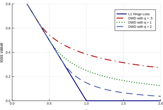
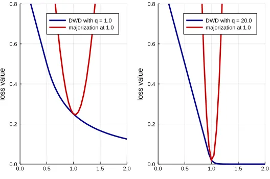
2.5.3 Generalized Distance Weighted Discrimination (DWD) . . . 42
2.5.4 Dirichlet-Multinomial MLE . . . 45
2.5.5 Quantile Regression . . . 46
2.6 Conclusion . . . 47
Chapter 3 Majorized Stochastic Proximal Iteration . . . 48
3.1 Introduction . . . 48
3.2 Majorized Stochastic Proximal Iteration . . . 50
3.2.1 Regularization . . . 52
3.3 Asymptotic Analysis . . . 54
3.3.1 Convergence for Smooth Nonconvex Objective . . . 59
3.4.1 Stability . . . 60
3.4.2 Finite Sample Bounds . . . 61
3.5 Examples . . . 67
3.5.1 Linear Regression . . . 67
3.5.2 Logistic Regression . . . 68
3.5.3 Distance Weighted Discrimination . . . 68
3.5.4 Quantile Regression . . . 69
3.6 Conclusion . . . 70
Chapter 4 OnlineStats.jl: Statistics for Streaming and Big Data . . . 71
4.1 Introduction . . . 71
4.1.1 Why Julia? . . . 73
4.2 Structure of OnlineStats . . . 73
4.2.1 OnlineStat . . . 73
4.2.2 Weight . . . 76
4.2.3 Series . . . 80
4.3 Stochastic Approximation Algorithms . . . 85
4.3.1 Stochastic Gradient Algorithms . . . 85
4.3.2 Stochastic MM Algorithms . . . 88
4.4 Algorithm Catalog . . . 91
4.4.1 Covariance Matrix (CovMatrix) . . . 91
4.4.2 Differences (Diff) . . . 92
4.4.3 Extrema (Extrema) . . . 93
4.4.4 Histograms (Hist) . . . 93
4.4.5 K-Means Clustering (KMeans) . . . 95
4.4.6 Linear Regression (LinReg and LinRegBuilder) . . . 95
4.4.7 Generalized Linear Models (StatLearn) . . . 98
4.4.8 Mean (Mean) . . . 100
4.4.9 Non-Central Moments (Moments) . . . 100
4.4.10 Order Statistics (OrderStats) . . . 101
4.4.11 Parametric Density Estimation . . . 102
4.4.12 Quantiles (Quantiles) . . . 107
4.4.13 Reservoir Sample (ReservoirSample) . . . 110
4.4.14 Sum (Sum) . . . 111
4.4.15 Variance (Variance) . . . 111
4.5 Extending OnlineStats . . . 112
4.5.1 User-Defined OnlineStat . . . 112
4.5.2 User-Defined Weight . . . 113
4.6 Conclusion . . . 113
5.1.1 Simulations . . . 115
5.2 Visualizations . . . 119
5.2.1 Linear Regression . . . 119
5.2.2 Logistic Regression . . . 121
5.2.3 Distance Weighted Discrimination . . . 123
5.2.4 Quantile Regression . . . 125
5.3 Conclusions . . . 127
LIST OF TABLES
LIST OF FIGURES
Figure 1.1 Convex Function . . . 5
Figure 1.2 Visualization of One MM Algorithm Iteration . . . 9
Figure 1.3 Coordinate Descent in Two Dimensions . . . 11
Figure 2.1 Visualization of One MM Algorithm Iteration . . . 23
Figure 2.2 “Contraction” term (1− 2µ/tr + 2R2/t2r) of SGD error bound with r =.7, R= 2, µ= 1. . . 39
Figure 2.3 DWD Losses compared with Hinge Loss (SVM) . . . 43
Figure 2.4 Quadratic Upper Bound for DWD Loss . . . 44
Figure 3.1 DWD Losses compared with Hinge Loss (SVM) . . . 69
Figure 4.1 Abstract OnlineStat Subtypes . . . 75
Figure 4.2 Equally-Weighted mean vs. Exponentially-Weighted Mean . . . 77
Figure 4.3 Weight Types Visualization . . . 80
Figure 4.4 Visualization of embarrassingly parallel computations in OnlineStats using themerge!function. . . 84
Figure 4.5 Visualization of One MM Iteration . . . 88
Figure 4.6 Quantile Loss forτ =.7 . . . 108
Figure 5.1 Legend for Learning Rate Parameters . . . 116
Figure 5.2 Linear Regression Simulation of 10 variables . . . 120
Figure 5.3 Linear Regression Simulation of 50 variables. . . 120
Figure 5.4 Logistic Regression Simulation of 10 variables . . . 122
Figure 5.5 Logistic Regression Simulation of 50 variables . . . 122
Figure 5.6 DWD Simulation forq=.5ofd = 10variables . . . 124
Figure 5.7 DWD Simulation forq= 20ofd= 10 variables . . . 124
Figure 5.8 Quantile Regression Simulation withτ = 0.7ofd= 10variables . . . 126
CHAPTER
1
INTRODUCTION
1.1
Preliminaries
The focus of this dissertation is online optimization applied to statistics. Anonline algo-rithmis one which accepts input sequentially, in contrast to anoffline algorithm where data is input all at once. However, not every online algorithm has an offline counterpart (and vice versa). As a trivial example, consider a sample mean ofn−1observations:
θ(noffline−1) = 1 n−1
n−1 ∑
i=1
xi. (1.1)
If a single new observation xnis included, an offline calculation revisits all of the
current estimate:
θ(n)offline= 1 n
n ∑
i=1
xi,
θ(n)online=
(
1− 1 n
)
θonline(n−1)+ 1 nxn.
(1.2)
As datasets in the age of big data get larger, so do the demands on traditional (of-fline) algorithms for fitting statistics and models. Online algorithms can naturally handle several forms of big data, such as files larger than computer memory (out-of-core pro-cessing) or observations arriving continuously in a stream (a common case in quanti-tative finance). However, the advantage of scaling to big data comes with drawbacks. Many model-fitting algorithms are iterative in nature because there does not exist a closed form solution, e.g. Newton’s method for logistic regression. In this case it is not possible for an online algorithm to fit a model to data as well as an offline counterpart; the objective function can be approximately minimized at best. The field of research involved with approximate objective function minimization is calledstochastic approxi-mation. While there has been increased interest in stochastic approximation in the last decade, there are still many open research questions and room for improvement over the state-of-the-art methods.
Contributions
The main contributions of this dissertation are threefold:
1. Several new methods of stochastic approximation that hold favorable properties over current methods.
2. A unified representation of online algorithms for statistics that can be executed in parallel, implemented in the OnlineStats.jl package.
3. A discussion of the difficulties in comparing stochastic approximation algorithms (ignored in the literature) as well as a novel visualization technique for examining robustness of algorithms to the choice of learning rate.
Notation
To fix notation, letθ ∈Rdrepresent a parameter vector of interest. For a given iterative
procedure, we denoteθ(t)as the estimated value after thet-th iteration. The objective
function we wish to minimize is ℓ(θ) :Rd → R. Denote the gradient (column-vector of
partial derivatives) as∇ℓ(θ) :Rd →Rd and the Hessian matrix asd2ℓ(θ) :Rd →Rd×d.
When a global minimum ofℓ(θ)exists, denote it asθ∗. LetDℓbe the domain of a function
ℓ(θ). The norm∥ · ∥is theL2 norm unless specified otherwise.
1.1.1
Statistical and Optimization Concepts
Types of ConvergenceStatistical consistency (convergence to the true population parameter) is an essential condition for an estimator to be valid. There are multiple notions of convergence for random variables. Three of them are discussed in this dissertation and are defined as follows.
Definition 1.1:Almost sure convergence (Xt a.s.
−−→X)
A random variable Xt convergesalmost surely (with probability 1) toX if
P
(
lim
t→∞Xt=X )
= 1. (1.3)
Definition 1.2:Convergence in probability (Xt p
− →X)
A random variable Xt convergesin probability toX if for everyϵ >0,
lim
t→∞P (|Xt−X|> ϵ) = 0. (1.4)
Definition 1.3:Convergence in distribution (Xt d
− →X)
A random variableXtconvergesin distributiontoX if for every bounded
contin-uous functionh,
lim
An important method for deriving the asymptotic distribution for a function of a ran-dom variable is called theDelta Method.
Theorem 1.4:Delta Method
(Casella and Berger, 2002) If a consistent estimatorθˆconverges in probability to the true valueθ∗ such that it has an asymptotic distribution
√
n(ˆθ−θ∗)−→d N(0,Σ), (1.6) the delta method implies that for a differentiable function f :Rd→Rk,
√
n[f(ˆθ)−f(θ∗)]−→d N(0,∇f(θ∗)TΣ∇f(θ∗)). (1.7)
Convexity
Convexity is a useful characteristic of a function often used in optimization. Below we give a mathematical definition of convexity as well as some properties of convex func-tions.
Definition 1.5:Convex Function
A functionf :U →Ris called convex if U is a convex set and
f[γθ1+ (1−γ)θ2]≤γf(θ1) + (1−γ)f(θ2) (1.8)
for0< γ < 1and for allθ1, θ2 ∈U. A function is calledstrictly convex if the above
inequality is strict.
Definition 1.6:Strong Convexity
A functionf :U →Ris calledM-strongly convex if f(θ1)≥f(θ2) +∇f(θ2)T(θ1−θ2) +
M
2 ∥θ1−θ2∥
2
2, for allθ1, θ2 ∈U. (1.9)
Proposition 1.7: Properties of Convex Functions
• (Supporting Hyperplane Inequality) A functionf is convex if and only if
f(θ1)≥f(θ2) +∇f(θ2)T(θ1−θ2), for allθ1, θ2 ∈Df. (1.10)
• (Second-order condition for convexity) A twice differentiable function f is convex if and only ifd2f(θ)is positive semi-definite for allθ ∈D
f.fis strictly
convex ifd2f(θ)is positive definite for allθ ∈Df.
• (Global optima) For a convex functionf onDf:
1. Any stationary point is a global minimum. 2. Any local minimum is a global minimum. 3. The set of global minima is convex.
4. Iff is strictly convex, the global minimum is unique. .
Figure 1.1: Convex Function
function lies beneath a straight line connecting any two points on the curve and it has a unique global minimum.
Lipschitz Continuity
A standard regularity condition isLipschitz Continuity. Definition 1.8:Lipschitz Continuity
A functionf :Rd →Ris calledL-Lipschitz continuous if
|f(θ1)−f(θ2)| ≤L∥θ1−θ2∥2, for allθ1, θ2 ∈Df. (1.11)
If L = 1, f is called a nonexpansivemapping. If L < 1, f is a contraction. When the gradient∇f isL-Lipschitz continuous, then
f(θ1)≤f(θ2) +∇f(θ2)T(θ1−θ2) +
L
2∥θ1−θ2∥
2
2, (1.12)
for all θ1, θ2 ∈ Df. This is a common assumption in convergence proofs of
optimiza-tion algorithms, as it implies there exists a quadratic upper bound of f. Therefore, if a functionf isM-strongly convex and has anL-Lipschitz continuous gradient, thenf is bounded between two quadratic functions.
1.2
Review of Offline Optimization
Newton’s Method
Newton’s method is the gold standard in optimization due to its fast (quadratic) con-vergence. Consider a second-order Taylor expansion around the current iterateθ(t) :
ℓ(θ)≈ℓ(θ(t)) +∇ℓ(θ(t))T(θ−θ(t)) + 1 2(θ−θ
(t))Td2ℓ(θ(t))(θ−θ(t)). (1.13)
Setting the gradient of this approximation equal to zero, we get updates of
The quadratic convergence and simplicity make Newton’s method an attractive candidate for optimization. However, the main drawback is that the calculation and inversion of the Hessian matrix d2ℓ(θ(t)) may be computationally expensive. Another
shortcoming is that iterations are not guaranteed to decrease the objective ℓ(θ). To remedy both situations, Newton’s method can be generalized to
θ(t+1) =θ(t)−st [
A(t)]−1∇ℓ(θ(t)), (1.15) where A(t) is a positive definite approximation ofd2ℓ(θ(t))and st is a step length. For
sufficiently small st, iterates are guaranteed to decrease ℓ(θ). Common choices for
the Hessian approximation areA=I (gradient descent) andA=E[d2ℓ(θ(t))](Fisher scoring method). If a numerical approximation ofd2ℓ(θ)is used rather than an analytical
one, this is called aQuasi-Newton method.
Expectation - Maximization (EM)
The EM algorithm has many applications in statistics as it provides the machinery for performing maximum likelihood estimation with unobserved or latent data. The latent data statistical model provides a unified framework which covers data with noise, miss-ing data, censored observations, and more (Dempster et al., 1977). EM differs from other algorithms in this review, since it is used to maximize a likelihood in contrast to minimizing a more general objective function.
Let Y be observed data and Z be missing or latent data that makes it easy to maximize the likelihood. Defineg(y, z|θ)as thecomplete data likelihood. The algorithm proceeds by alternating between an expectation step and a maximization step.
• Expectation Step
Evaluate the expectation (with respect to the latent data) of the complete data likelihood, conditioned on the parameter being equal to the current estimate:
Q(θ|θ(t+1)) = EZ[lng(Y, Z|θ)Y =y, θ=θ(t)] (1.16)
• Maximization Step
The EM algorithm is very stable as each iteration is guaranteed to increase the (observed data) likelihood.
Majorization - Minimization (MM)
The MM algorithm is more of a concept than an actual algorithm. Suppose it is difficult or costly to minimize an objectiveℓ(θ)directly. The MM concept is to iteratively create majorizing functions and minimize them. MM is extremely stable, as each iteration is guaranteed to decrease the objective. This is similar to the EM algorithm’s guaran-teed ascent property, due to the fact that EM is a special case of MM. The advantage over EM is that a wider class of problems that can be solved; the objective function does not need to be a likelihood and the majorizing technique does not need to be an expectation.
• Majorization Step
Construct a functiong(θ|θ(t))such that
g(θ|θ(t)) ≥ ℓ(θ), for allθ (dominance condition), g(θ(t)|θ(t)) = ℓ(θ(t)) (tangent condition).
(1.18)
• Minimization Step
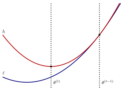
θ(t+1) =arg min
θ
Figure 1.2: Visualization of One MM Algorithm Iteration
The above figure demonstrates a single MM iteration in one dimension. Beginning atθ(t−1), the majorizing step creates the red line. Then, the minimization step finds the
red line’s minimizer, which movesθ(t−1) to θ(t). Therefore, the MM iteration moves the
estimate in the correct direction of the global minimizer.
The key to efficient MM algorithms, constructing majorizations, is a bit of an art form. Hunter and Lange (2004) provide several techniques for creating majorizations:
• Jensen’s Inequality
For a convex functionℓ and random variableX, Jensen’s inequality states that
ℓ[E(X)]≤E[ℓ(X)]. (1.20)
For probability densitiesa(x), b(x), the fact that−ln(x)is convex can be used to conclude
−ln
{
E
[
a(X) b(X)
]}
≤ −E
{
ln
[
a(X) b(X)
]}
. (1.21)
IfX has densityb(x), the following inequality can be derived:
It is this fact that shows the minorizing property of the E-step in the EM algorithm. • Minorization via Supporting Hyperplanes
Ifℓis convex and differentiable,
ℓ(θ)≥ℓ(θ(t)) +∇ℓ(θ(t))T(θ−θ(t)), (1.23) with equality atθ=θ(t). Thus, the right-hand side is a minorization.
• Majorization via the Definition of Convexity A functionℓis convex if and only if
f
( ∑
i
αiti )
≤∑
i
αif(ti) (1.24)
for a finite collection of pointstiand nonnegative multipliersαisuch that ∑
iαi =
1. Whenℓis composed with a linear functionxTθ, substitutingt
i =xi(θi−θ (t) i )/αi+
xTθ(t) creates the inequality (De Pierro, 1995)
ℓ(xTθ)≤∑
i
αiℓ [
xi
αi
(θi−θi(t)) +x T
θ(t)
]
. (1.25)
• Majorization via Quadratic Upper Bound
Supposeℓis twice differentiable and there exists a matrixM such thatM−d2ℓ(θ)
is positive semi-definite for allθ. Then there exists a quadratic upper bound
ℓ(θ)≤ℓ(θ(t)) +∇ℓ(θ(t))T(θ−θ(t)) + 1 2(θ−θ
(t))TM(θ−θ(t)). (1.26)
Minimizing the right-hand side results in Newton-like updates where the Hessian matrix is replaced withM:
Coordinate Descent
Coordinate descent algorithms minimize the objective function with respect to one el-ement at a time while keeping the others constant.
θj(t+1) =arg min
θj ℓ
(
θ(t+1)1 , . . . , θj(t+1)−1 , θj, θ (t)
j+1, . . . , θ (t) p
)
(1.28)
forj = 1, . . . , p.
θ2
θ1
Figure 1.3: Coordinate Descent in Two Dimensions
The figure above demonstrates coordinate descent in two dimensions using a smooth, strongly convex objective. Coordinate descent also has the descent prop-erty, but is not guaranteed to converge for a non-differentiable objective. However, it will converge to a global minimum for an objective ℓ(θ) = f(θ) +g(θ) wheref is con-vex and differentiable and g is convex. This makes coordinate descent well suited to generalized linear models with regularization (Friedman et al., 2010).
Proximal Gradient Method
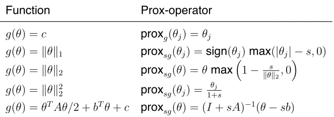
Definition 1.9:Prox Operator
The prox operator or proximal mapping of a convex function g with scalingsis
proxsg(θ) = arg min
u (
g(u) + 1
2s∥u−θ∥
2 )
. (1.29)
Intuitively, the mapping is a compromise between minimizingg and remaining nearθ, where the scalings controls the amount of tradeoff. Also note that the function being minimized by the proximal mapping is a majorizing function of g, so a prox step is an MM update.
Table 1.1: Prox-operator Examples
Function Prox-operator g(θ) = c proxg(θj) = θj
g(θ) = ∥θ∥1 proxsg(θj) = sign(θj)max(|θj| −s,0)
g(θ) = ∥θ∥2 proxsg(θ) = θmax (
1−∥θs∥ 2,0
)
g(θ) = ∥θ∥2
2 proxsg(θj) =
θj
1+s
g(θ) = θTAθ/2 +bTθ+c prox
sg(θ) = (I +sA)−1(θ−sb)
The proximal gradient method minimizes a function with two components
ℓ(θ) = f(θ) +g(θ), (1.30)
wherefis convex and differentiable andgis a closed convex function with inexpensive prox operator. Iterates take the form
θ(t+1)=arg min
θ {
f(θ(t))− ∇f(θ(t))T(θ+θ(t)) + 1 2st
∥θ−θ(t)∥2+g(θ)
}
=proxs
tg
(
θ(t)−st∇f(θ(t)) )
.
Thus, the update alternates between a gradient descent step with respect to the differentiable function f and performing a proximal mapping with respect to g. Ifst <
1/L and f(θ) has an L-Lipschitz continuous gradient, a proximal gradient step is an MM step.
Beck and Teboulle (2009) introduced the Fast Iterative Shrinkage-Thresholding Al-gorithm (FISTA), an accelerated proximal gradient method. The idea is to perform prox-imal gradient steps on an extrapolated point.
y =θ(t)+t−2 t+ 1
(
θ(t)−θ(t−1)), θ(t+1) =proxsg(y−s∇f(y)).
(1.32)
1.3
Review of Online Optimization
Online optimization is almost synonymous with stochastic approximation. Consider the common machine learning objective to minimize an expected loss with respect to an unknown random variable:
arg min
θ
EY[ℓ(Y, θ)]. (1.33)
An online algorithm will update parameter estimatesθ(t)based on the previous iterate θ(t−1) and a random sample yt ∼Y, so the updater has access to all information
con-tained in ℓ(yt, θ). Some stochastic algorithms are not online, but take random draws
of observations from a fixed size dataset. Popular examples of this are the algorithms SAG (Schmidt et al., 2017), SAGA (Defazio et al., 2014), SVRG (Johnson and Zhang, 2013), and MISO (Mairal, 2015). These algorithms follow the form of (1.33) by replacing Y with the empirical distribution of a sample.
1.3.1
Stochastic Approximation
Robbins-Monro Algorithmhere. Suppose we wish to use successive approximations θ(t) to find the unique root
θ∗ of a functionM(θ)based on observations
yt=M(θ(t−1)) +ϵt, (1.34)
whereϵtare unobservable random errors with mean 0. The Robbins-Monro algorithm
is
θ(t) =θ(t−1)−γtyt,
=θ(t−1)−γt [
M(θ(t−1)) +ϵt
] (1.35)
where{γt}∞t=1is a positive sequence such that ∑
γt =∞, ∑
γ2
t <∞. Convergence to
θ∗ is achieved under the assumptionM(θ(t))>0whenθ(t) > θ∗ andM(θ(t))<0when
θ(t) < θ∗.
Kiefer-Wolfowitz Algorithm
For finding a critical point of a function, the Robbins-Monro algorithm is modified by Kiefer and Wolfowitz (1952) to use updates of the form
θ(t)=θ(t−1)−γt [
yt(θ(t−1)+ct)−yt(θ(t−1)−ct)
2ct
]
, (1.36)
wherectis a positive sequence such that ∑
γtct<∞. In other words, the derivative is
estimated with finite differences.
The approach to prove convergence used by Robbins and Monro (1951) and Kiefer and Wolfowitz (1952) starts with showingE[(θ(t)−θ∗)2]converges to some limit inL2.
Then, a contradiction is found ifθ(t)does not converge toθ∗ in probability. Blum (1954) proved almost sure convergence for the Robbins-Monro under assumptions
|M(θ(t))| ≤c(|θ(t)−θ∗|+ 1) for allθ(t) and somec >0, inf
ϵ≤|θ(t)−θ|≤1/ϵ
[
M(θ(t))(θ(t)−θ∗)]>0 for all0< ϵ <1, (1.37) and almost sure convergence for Kiefer-Wolfowitz after removing the assumption
∑
Nonnegative Almost Supermartingale
A concept that appears in convergence proofs of stochastic approximation algorithms is the idea of afiltration. A filtration can be interpreted as the formal concept of history or past information.
Definition 1.10:Filtration
Let(Ω,F, P)be a probability space withσ-algebraF and probability measureP. A filtration is an increasing sequence ofσ-algebras
F1 ⊂ F2 ⊂. . .⊂ F. (1.38)
A sequence of random variablesXtalways has the natural filtration whereFt=
σ(X1, . . . , Xt) is the σ-algebra generated by the random sequence up to t. By
property of Ft-measurable random variables, E(Xt|Ft) = Xt. IfE(|Xt|) <∞ for
all t and E[Xt|Fs] = Xs for all s < t, {Xt}is said to be adapted to the filtration
{Ft}.
Definition 1.11:Nonnegative Almost Supermartingale
Suppose there exists nonnegative Ft-measurable random variables Mt, At,Bt,Ct such that
E(Mt+1|Ft)≤(1 +At)Mt−Bt+Ct. (1.39)
If∑At<∞and ∑
Ct<∞almost surely, thenMtconverges to a finite limit and ∑
Bt<∞almost surely. A sequence that satisfies (1.39) is called anonnegative
almost supermartingale.
Robbins and Siegmund (1985) proved convergence of the Robbins-Monro algo-rithm using almost supermartingale theory withMt= (θ(t)−θ∗)2.
Connection with Ordinary Differential Equations
Robbins-Monro updates with an ordinary differential equation. Let st = ∑t
i=1γi be the sum
of weights up until pointt. The updates can then be interpreted as a function of “time”. Define
θ(s) = θ
(t)(s
t+1−s) +θ(t+1)(s−st)
st+1−st
, st≤s < st+1. (1.40)
That is,θ(st) = θ(t)andθ(s)is the linear interpolation betweenθ(t), θ(t+1)whenst< s <
st+1. Rearranging the Robbins Monro update (1.35) and rewriting estimates as above,
we get
θ(t) =θ(t−1)−γt[M(θ(t−1)) +ϵt],
θ(t)−θ(t−1)
γt
=−M(θ(t−1))−ϵt,
θ(st)−θ(st−1)
st−st−1
=−M(θ(st−1))−ϵt.
(1.41)
Sincest−st−1 =γt→0, this is strikingly similar to the ordinary differential equation
dθ
ds =−M[θ(s)]. (1.42)
Under regularity conditions, θ(t) →θ∗ ifθ∗ is a global asymptotically stable equilibrium of the ODE. For technical details, we refer the reader to Kushner and Yin (2003).
Stochastic Gradient Descent (SGD)
Stochastic gradient descent was introduced by Sakrison (1965) and is a straightforward application of the Robbins-Monro algorithm. It is fairly intuitive and easy to implement for a wide variety of optimization problems. In recent years, SGD-like algorithms have been popular for online machine learning problems as it is trivially scalable to big data. Putting SGD in the Robbins-Monro form, we wish to solveM(θ) =EY[∇ℓ(Y, θ)] = 0. This expectation cannot be observed, but we can obtainM(θ)+ϵtwhereϵt =∇ℓ(yt, θ)−
M(θ)andytare random samples from the distribution ofY. The updates are then
Asymptotic Normality
Chung (1954) and Sacks (1958) were the first to investigate the asymptotic distri-bution for the Robbins-Monro algorithm. Under the learning rate γt = (tβ)−1 where
β =M′(θ∗), the univariate Robbins-Monro iterates satisfy √
t(θ(t)−θ∗)→N
(
0,σ
2
β2 )
, (1.44)
whereσ2 =limt→∞E(ϵt|Ft−1). The extension to the multivariate case is given in Fabian (1968).
More recently, Toulis et al. (2017) derived asymptotic normality for a variety of stochastic gradient updates of the form
θ(t)=θ(t−1)−γtCt∇ℓt(θ(t−1)), (1.45)
whereℓt(θ) =ℓ(yt, θ),γt>0andCt is a positive definite matrix.
Assumption 1.12: Assumptions for Normality of Stochastic Gradient Update (a) The step size sequence isγt=η/tr, η >0, r ∈(0.5,1].
(b) The objectiveℓ(θ)is convex,L-Lipschitz continuous, twice differentiable, and minimized atθ∗.
(c) The Hessian matrix for online objectives have positive trace for allt:
trace[d2ℓt(θ)] > 0. The eigenvalues of the expected second derivative are
bounded:0< λj <∞for all eigenvaluesλj ofE[d2ℓt(θ)].
(d) Each matrixCtis a positive definite matrix such thatCt=C+O(γt)whereCis
symmetric, positive definite and commutes withE[d2ℓ(θ∗)]. The eigenvalues
of eachCt are bounded:0< λtj <∞for all eigenvaluesλtj ofCt.
(e) The Lindeberg conditions for asymptotical normality are satisfied. Let
Ξt=E[∇ℓt(θ∗)∇ℓt(θ∗)T|Ft−1]. Then∥Ξt−Ξ∥=O(1)for allt, and∥Ξt−Ξ∥ →0
for a symmetric positive definite matrixΞ. Letσ2t,s=E[1∥ξt(θ∗)∥2≥s/γ
t∥ξt(θ∗)∥
2].
Theorem 1.13:Asymptotic Normality of Stochastic Gradient Algorithms
Under the above assumptions wherer= 1and2ηCd2ℓ(θ∗)−Iis positive definite,
the updatesθ(t)from (1.45) are asymptotically normal with meanθ∗and variance
η2[2ηCd2ℓ(θ∗)−I]−1Cd2ℓ(θ∗)C
t . (1.46)
Polyak-Ruppert Averaging
While not an algorithm itself, averaging techniques (Polyak and Juditsky, 1992; Rup-pert, 1988) can often accelerate convergence of stochastic approximation methods. The motivating idea is that averaging the iterates reduces variability. In practice, it is common to let the algorithm learn for a finite number of samples t0 and then begin
averaging:
¯
θ(t)= 1 t−t0
t ∑
i=t0
θ(i). (1.47)
Online EM Algorithm
An online version of the EM algorithm in Cappé and Moulines (2009) is based on min-imizing a stochastic approximation of the expectation step. To ease the transition to the online case, here we present the (offline) EM algorithm in a slightly different form. Assume the negative loglikelihood is normalized byn, the number of observations:
ℓ(θ) = 1 n
n ∑
i=1
ℓi(θ), (1.48)
so thatℓ(θ)is majorized by
Qt(θ) =
1 n
n ∑
i=1
gi(θ|θ(t−1)), (1.49)
be written as
Qt(θ) =
1 n
n ∑
i=1
gi(θ|θ(t−1)),
θ(t) =arg min
θ
Qt(θ).
(1.50)
For the online EM algorithm, we observe a sequence of independent random sam-ples yt. For each sample, a majorizing expectation is created such that g(yt, θ|θ(t−1))
majorizesℓ(yt, θ)atθ(t−1). The online EM algorithm then performs the updates
Qt(θ) = (1−γt)Qt−1(θ) +γtg(yt, θ|θ(t−1)),
θ(t) =arg min
θ
Qt(θ),
(1.51)
where{γt}∞t=1 satisfies ∑
γt = ∞, ∑
γ2
t < ∞. The proof of consistency in Cappé and
Moulines (2009) relies on assuming the complete data likelihood comes from an expo-nential family. The stochastic approximation (E) step thus amounts to approximating the sufficient statistics from the complete data likelihood.
1.4
Discussion
Many of the offline algorithms in this chapter have stochastic approximation counter-parts. Just as Newton’s method is the gold standard for offline optimization, stochastic gradient descent (the online counterpart to gradient descent) is the gold standard for online optimization. Most of the recent developments in online optimization are variants of SGD. The main drawback to SGD-like algorithms is that there is information “left on the table” at each update. By only using gradient information, there is no guarantee of reducing the objective function for even the current observation. The first few iter-ations of stochastic gradient algorithms often do more harm than good, forcing future iterations to “undo damage” before converging to the correct solution. One can ensure stability in finite samples with a careful selection of hyper-parameters (step size se-quence{γt}), but this adds complexity to already-complex methods. This dissertation
second-less sensitive to step sizes. Little has been done to incorporate the MM algorithm into the world of stochastic approximation, but this dissertation shows there is much to be gained by doing so.
CHAPTER
2
ONLINE MM ALGORITHMS
2.1
Introduction
In the online learning setting, the goal is to find
arg min
θ
EY[ℓ(Y, θ)], (2.1)
where the expectation cannot be evaluated, but the learner has access to a sequence of random samples{yt}∞t=1fromY. A learner updates the estimateθ(t)from the sample
yt and the previous estimateθ(t−1) using the information contained in ℓt(θ) = ℓ(yt, θ).
Many online learning algorithms are variants of stochastic gradient descent (SGD), which is defined by minimizing a quadratic approximation for a positive step sizeγt:
θ(t) =arg min
θ {
ℓt(θ(t−1)) +∇ℓt(θ(t−1))T(θ−θ(t−1)) +
1 2γt
∥θ−θ(t−1)∥2
}
=θ(t−1)−γt∇ℓt(θ(t−1)).
(2.2)
Since SGD-like algorithms use only the gradient, all other information contained in ℓt(θ) is ignored. The algorithms introduced in this chapter naturally incorporate more
MM Algorithms
The MM algorithm is more of a concept than it is an actual algorithm. Suppose it is difficult or costly to minimize an objectiveℓ(θ)directly. The MM concept is to iteratively create majorizing functions and minimize them. MM is extremely stable, as each itera-tion is guaranteed to decrease the objective. As a generalizaitera-tion of the EM algorithm, the objective function does not need to be a likelihood and the majorizing technique does not need to be an expectation. An introduction to (offline) MM algorithms is given in Hunter and Lange (2004), with a more thorough treatment in Lange (2016).
• Majorization Step
Construct a surrogate objective functionhsuch that
h(θ|θ(t−1))≥ℓ(θ), with strict equality atθ =θ(t−1). (2.3)
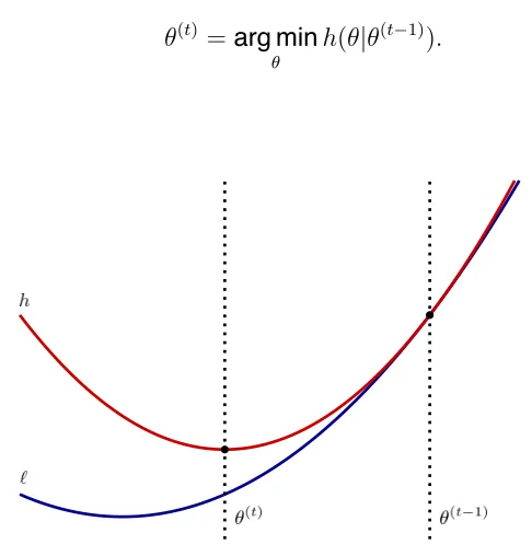
• Minimization Step Minimizeh:
θ(t) =arg min
θ
h(θ|θ(t−1)). (2.4)
The figure above shows the descent property of MM algorithms: By minimizing a surrogate functionh, the estimate moves closer to the optimal value ofl. The surrogate hincorporates some of the second order information ofland therefore guarantees that the update doesn’t “jump too far”.
Constructing majorizing functions is a bit of an art form. A common method of con-struction is via a quadratic upper bound (Hunter and Lange, 2004). Letℓ(θ)be a twice differentiable objective function and suppose there exists a matrixAsuch thatA−d2ℓ(θ) is positive semi-definite. Then, the function
h(θ|θ(t)) =ℓ(θ(t)) +∇ℓ(θ(t))T(θ−θ(t)) + 1 2(θ−θ
(t)
)TA(θ−θ(t)) (2.5) majorizesℓ(θ)atθ(t). Minimizing this surrogate creates updates of the form
θ(t) =θ(t−1)−γtA−1∇ℓ(θ(t−1)). (2.6)
Therefore, quadratic upper bound MM updates look similar to Newton’s method, but use an approximation of the Hessian matrix that guarantees descent. Note that if A is diagonal, updates can be performed element by element, and it is not necessary to solve a linear system at each iteration. Furthermore, ifℓ(θ)has anL-Lipschitz contin-uous gradient and I is the identity matrix of appropriate size, LI −d2ℓ(θ) is positive
semi-definite and A=LI can be used in the majorization.
The following two propositions are useful in constructing quadratic upper bounds for models that are linear in the parameters, i.e. the objective has the formℓt(θ) = ft(xTtθ).
In this case, the second derivative isft′′(xTtθ)xtxTt. Therefore, ifft′′(xTtθ)is bounded for
all θ for some constant c and A −xtxTt is positive semidefinite, then cA−d2ℓt(θ) is
Proposition 2.1
Let diag(A) denote the diagonal matrix containing the diagonal elements of A. For a matrix X = (x1, x2, . . . , xp)∈ Rn×p, pdiag(XTX)−XTX is positive
semi-definite.
Proof. Leta∈Rp. LetX = (x
1, x2, . . . , xp). Then
aT[pdiag(XTX)−XTX]a =p aTdiag(XTX)a−aTXTXa =p
p ∑
j=1
a2jxTjxj − p ∑ i=1 p ∑ j=1
aiajxTi xj
=p
p ∑
j=1
∥vj∥2− p ∑ i=1 p ∑ j=1
viTvj forvi =aixi
= (p−1)
p ∑
j=1
∥vj∥2−2 p ∑
i=1 ∑
j>i
viTvj
= p ∑ i=1 ∑ j>i [
(∥vi∥ − ∥vj∥) 2
+ 2∥vi∥∥vj∥ ] −2 p ∑ i=1 ∑ j>i
viTvj
≥ p ∑ j=1 ∑ i>j
2∥vi∥∥vj∥ −2vTi vj
Proposition 2.2
Forx∈Rd,xTxI−xxT is positive semi-definite. Proof. Leta∈Rd. Then
aT(xTxI−xxT)a =aTxTxIa−aTxxTa =ataxTx−aTxxTa =∥a∥2∥x∥2−(aTx)2
≥0 by Cauchy-Schwarz inequality.
(2.7)
Online EM Algorithm
The (offline) EM algorithm, introduced in Dempster et al. (1977), has a wide variety of uses in statistics, signal processing, and optimization. The EM idea assumes there is some unobserved or missing data Z that if observed would make the maximum likelihood estimate (MLE) easy to calculate. LetY be the observed data andf(Y, Z|θ) be the complete data probability density function parameterized by θ. As a specific case of MM, the offline EM algorithm alternates between an expectation (minorization) step and a maximization step. Note that when the objective is maximizing an objective function, MM stands for Minorize-Maximize instead of Majorize-Minimize. To keep the EM algorithm consistent with the algorithms in this chapter (in terms of minimization), we alter the EM update to use the negative loglikelihood:
Qt(θ) =
1 n
n ∑
i=1
EZ[−lnf(yi, zi|θ)|θ(t−1) ]
,
θ(t)=arg min
θ
Qt(θ).
(2.8)
The precursor to Stochastic MM is the online EM algorithm in Cappé and Moulines (2009), based on a stochastic approximation of the expectation:
Qt(θ) = (1−γt)Qt−1(θ) +γtEZ[−ln(yt, zt|θ)|θ(t−1)],
θ(t) =arg minQt(θ),
where γt ∈ (0,1). Therefore, in translating the EM algorithm to an online update, the
M-step remains the same, but the expectation step must use an approximation since only a single observation is available.
2.2
Online MM Algorithms
The two presented algorithms will be jointly referred to as online MM algorithms, as the updates are based on majorizations and behave similarly in both theory and prac-tice. For each algorithm, the update is defined in terms of step size γt ∈ (0,1) and
ht(θ) =h(yt, θ|θ(t−1)), a known function of the current iterate and new observation that
majorizesℓt(θ) =ℓ(yt, θ)atθ(t−1).
2.2.1
Online MM - Averaged Surrogate (OMAS)
Mairal (2013b) introduced the following algorithm asStochastic MM, in which the online EM algorithm is extended to MM algorithms by directly replacing the expectation in equation (2.9) with a more general majorization. The OMAS update is then
Qt(θ) = (1−γt)Qt−1(θ) +γtht(θ)
θ(t) =arg min
θ
Qt(θ).
(2.10)
2.2.2
Online MM - Averaged Parameter (OMAP)
Rather than averaging surrogate functions, OMAP averages the arguments that min-imize the majorizations. Therefore, OMAP is only well-defined for majorizations that have a unique minimum:
θ(t) = (1−γt)θ(t−1)+γtarg min θ
2.2.3
Online MM via Quadratic Upper Bound
Recall that majorization via a quadratic upper bound is a common method of con-structing surrogates. Ifℓ(θ)is twice differentiable and there exists a matrixAsuch that A−d2ℓ(θ)is positive semi-definite for allθ, the function
h(θ|θ(t−1)) =ℓ(θ(t−1)) +∇f(θ(t−1))T(θ−θ(t−1)) + 1 2(θ−θ
(t−1)
)TA(θ−θ(t−1)) = 1
2θ
THθ+ [∇f(θ(t−1))−Hθ(t−1)]Tθ+c,
(2.12)
where c includes all the terms that do not depend on θ, majorizes ℓ(θ) at θ(t−1).
For-tunately, closed-form updates can be derived for OMAS and OMAP. This makes it straightforward to translate existing offline MM algorithms via quadratic upper bound into online updates. Updates of this form will be referred to as OMAS-Q and OMAP-Q, respectively.
• OMAS-Q
At= (1−γt)At−1+γtHt,
bt= (1−γt)bt−1 +γt[Htθ(t−1) − ∇ℓt(θ(t−1))],
θ(t) =A−t1bt.
(2.13)
• OMAP-Q
θ(t) =θ(t−1)−γtHt−1∇ℓt(θ(t−1)). (2.14)
The difference between OMAS and OMAP is clearly seen in the above updates: OMAS consists of updating “sufficient statistics” while OMAP is directly applied to the parameter.
2.2.4
Regularization in OMAS-Q and OMAP-Q
In machine learning, the objectivesℓt(θ)often have the formℓt(θ) =ft(θ) +λψ(θ), (2.15)
size of the coefficients θ, and λ ≥ 0is a tuning parameter that adjusts the amount of regularization.
Note that majorizing ℓt(θ) is possible by majorizing the loss component only and
leaving the penalty function as-is. Letht(θ)majorizeft(θ)atθ(t−1). Then
ht(θ) +λψ(θ) (2.16)
majorizes ℓt(θ) atθ(t−1). Therefore, it is trivial to add a regularization term into a
ma-jorization. The second part of MM, minimization, is also straightforward in the case of OMAS-Q and OMAP-Q. First consider OMAP-Q where∇ℓ(θ)isL-Lipschitz continuous and the Hessian matrix approximation isLIfor the identity matrixIof appropriate size. The update is then
θ(t)= (1−γt)θ(t−1)+γtarg min θ
{
∇ℓt(θ(t−1))Tθ+
L 2∥θ−θ
(t−1)∥2+λψ(θ) }
= (1−γt)θ(t−1)+γtproxλ Lψ
[
θ(t−1)− 1 L∇ℓt(θ
(t−1)) ]
,
(2.17)
where theprox operator orproximal mapping is defined as
proxψ(u) = arg min
θ {
ψ(θ) + 1
2∥u−θ∥
2 }
. (2.18)
Therefore, the second term in (2.17) is using a proximal gradient step (Parikh et al., 2014) applied to the noisy objective ℓt(θ). Now consider OMAS-Q with the same
ma-jorization:
Qt(θ) = (1−γt)Qt−1(θ) +γtht(θ),
θ(t) =arg min
θ
{Qt(θ) +λψ(θ)}
=arg min
θ {
LθTθ/2−btθ+λψ(θ) }
=arg min
θ {
λψ(θ) + L 2
θ− bt
L
2
}
wherebt = (1−γt)bt−1+γtL[θ(t−1)− ∇ft(θ(t−1))].
Regularized OMAS-Q has an advantage over regularized OMAP-Q in regard to variable selection. The prox step for certain penalties (such as LASSO) sets small coefficients equal to zero. OMAP-Q coefficients will only be zero if they are zero in every iteration, since the prox step occurs before the averaging occurs. In OMAS-Q, the prox step occurs after averaging and thus coefficients can be set to zero during any iteration.
2.3
Asymptotic Analysis
Most theoretical guarantees for online learning algorithms are based on convex ob-jectives only. In this section, we show online MM algorithms are not only consistent in the convex case, but converge to a critical point for nonconvex objectives. The theory shows online MM algorithms take steps that are correlated with the stochastic gradi-ent, but naturally incorporate second order information from the stochastic objective. As the stochastic gradient is used often in the following analysis, letgt = ∇ℓt(θ(t−1))
with elements gt = (gt1, . . . , gtd). Online MM algorithms will be interpreted to take the
formθ(t) =θ(t−1)−γ
tδt, where the “direction” vector has elementsδt= (δt1, . . . , δtd).
Convergence of online MM algorithms rely on the theory of nonnegative almost supermartingales, discussed in Robbins and Siegmund (1985). The main result is pre-sented below as a lemma.
Lemma 2.3:Almost Supermartingale Convergence
Suppose there exists sequences of nonnegative random variables At, Bt, and
Ct, adapted to filtration Ft, such that
E[Mt+1|Ft]≤(1 +At)Mt−Bt+Ct. (2.20)
If∑At<∞and ∑
Ct<∞almost surely, thenMtconverges to a finite limit and ∑
Assumption 2.4: Online MM Algorithm Assumptions (a) The step size sequence satisfies
γ1 = 1,
0< γt<1ift >1, ∑
γt=∞, ∑
γt2 <∞.
(2.21)
(b) For allt, the stochastic majorizing functionsht have anL-Lipschitz
continu-ous gradient and areM-strongly convex. Necessarily,M ≤L. There exists a constantB >0such that∥gt∥2 ≤B for allt.
(c) Each element of the online MM direction vector satisfies sign(δtj) =sign(gtj)
and|δtj| ≥c|gtj|for somec >0.
(d) The parameter space is a convex open subset Θ ⊂ Rd. arg minθht(θ) ∈ Θ
for allt, the data sequence{yt}∞t=1is independent and identically distributed,
andℓ(y, θ)is well defined for all(y, θ)∈ Y ×Θ.
In assumption 2.4, The first two parts of (a) ensure that Q1(θ) = ht(θ) and that
iterates remain inside the parameter space. The second two conditions are standard assumptions for stochastic approximation. Assumption (b) puts regularity conditions on the majorizations that are common in practice. Assumption (c) may at first appear to be a strong condition, but it is satisfied for any majorization that splits parameters into a separable sum
ht(θ) = d ∑
j=1
htj(θj), (2.22)
where each component htj is M-strongly convex and has an L-Lipschitz continuous
gradient for a sufficiently largeL.
time, but online MM algorithms do follow astochastic descent property. Proposition 2.5: Stochastic Descent Property
Online MM algorithms satisfy the stochastic descent property for all t and any step sizeγt ∈(0,1):
ℓ(yt, θ(t))≤ℓ(yt, θ(t−1)). (2.23)
Proof. For OMAS,
Qt(θ(t))≤Qt(θ(t−1))
(1−γt)Qt−1(θ(t)) +γtht(θ(t))≤(1−γt)Qt−1(θ(t−1)) +γtht(θ(t−1))
(1−γt)Qt−1(θ(t)) +γtht(θ(t))≤(1−γt)Qt−1(θ(t)) +γtht(θ(t−1))
ht(θ(t))≤ht(θ(t−1))
ℓt(θ(t))≤ht(θ(t))≤ht(θ(t−1)) =ℓt(θ(t−1)).
(2.24)
For OMAP, by definition of majorization and convexity,
ℓt(θ(t))≤ht(θ(t))
=ht[(1−γt)θ(t−1)+γtarg min θ
ht(θ)]
≤(1−γt)ht(θ(t−1)) +γtminh(θ)
≤(1−γt)ht(θ(t−1)) +γtht(θ(t−1))
=ht(θ(t−1))
=ℓt(θ(t−1)).
(2.25)
Lemma 2.6:Properties of OMAS Surrogates
Under assumption 2.4 (b), Qt(θ) isM-strongly convex with an L-Lipschitz
con-tinuous gradient for all t. Furthermore,
∇Qt(θ(t−1)) = γtgt. (2.26)
Proof. The Lipschitz condition and strong convexity are both proven by induction. Q1(θ) = h1(θ) has an L-Lipschitz continuous gradient. Assume ∇Qt−1 is L
-Lipschitz continuous. ThenQt(θ)has anL-Lipschitz continuous gradient by
def-inition:
∥∇Qt(θ1)− ∇Qt(θ2)∥ ≤(1−γt)∥∇Qt−1(θ1)− ∇Qt−1(θ2)∥+γt∥∇ht(θ1)− ∇ht(θ2)∥
≤(1−γt)L∥θ1−θ2∥+γtL∥θ1−θ2∥
=L∥θ1−θ2∥,
(2.27) Q1(θ) = h1(θ) is M-strongly convex. AssumeQt−1(θ) is M-strongly convex, so
by definitionQt−1(θ)− M2 θTθ is convex. Then
Qt(θ)−
M 2 θ
T
θ = (1−γt) [
Qt−1(θ)−
M 2 θ
T
θ
]
+γt [
ht(θ)−
M 2 θ
T
θ
]
(2.28)
is a weighted average of convex functions andQt(θ)is convex by definition.
Lemma 2.7:Online MM Update Bounds
Under assumption 2.4, online MM iterates satisfy γt2
L2∥gt∥
2 ≤ ∥θ(t−1)−θ(t)∥2 ≤ γ 2 t
M2∥gt∥
2, (2.29)
and therefore converge to a finite point almost surely.
Proof. For OMAS,Qt(θ)isM-strongly convex and has anL-Lipschitz continuous
gradient. Therefore, 1
L2∥∇Qt(θ (t−1)
)∥2 ≤ ∥θ(t−1)−θ(t)∥2 ≤ 1
M2∥∇Qt(θ (t−1)
)∥2, 1
L2∥gt∥
2 ≤ ∥
θ(t−1)−θ(t)∥2 ≤ 1 M2∥gt∥
2
.
(2.30)
For OMAP,∥θ(t−1)−θ(t)∥2 =γ2
t∥arg minθht(θ)−θ(t−1)∥2. Sinceht(θ)isM-strongly
convex and has an L-Lipschitz continuous gradient, γt2
L2∥gt∥ 2 ≤
γt2∥arg min
θ
ht(θ)−θ(t−1)∥2 ≤
γt2 M2∥gt∥
2
. (2.31)
In both cases, limt→∞∥θ(t−1)−θ(t)∥2 = 0, so it must be thatθ(t) →θ(∞) for some finite valueθ(∞) almost surely.
A result of the above lemma is that by writing online MM iterates as
θ(t)=θ(t−1)−γtδt, (2.32)
the direction vector δt satisfiesL−1∥gt∥ ≤ ∥δt∥ ≤ M−1∥gt∥. This direction can be
ex-plicitly derived for both OMAS and OMAP:
δtOM AS = θ
(t−1)−arg min
θQt(θ)
γt
, δtOM AP =θ(t−1)−arg min
θ
ht(θ).
Lemma 2.8:Online MM Direction and Stochastic Gradient
The update direction is positively correlated withgt =∇ℓt(θ(t−1))for allt.
Specif-ically,
γt
L∥gt∥
2 ≤gT
t (θ(t−1)−θ(t))≤
γt
M∥gt∥
2. (2.34)
In other words,
1 L∥gt∥
2 ≤
gtTδt ≤
1 M∥gt∥
2
. (2.35)
Proof. For OMAS,Qt(θ)is convex and has anL-Lipschitz gradient, which implies
co-coercivity of the gradient:
[
∇Qt(θ(t−1))− ∇Qt(θ(t)) ]T
(θ(t−1)−θ(t))≥ 1
L∥∇Qt(θ
(t−1))− ∇Q
t(θ(t))∥2
γtgtT(θ (t−1)−
θ(t))≥ γ
2 t
L∥gt∥
2
.
(2.36)
Similarly for OMAP:
gtT(θ(t−1)−θ(t)) =γtgtT[θ
(t−1)−arg min θ
ht(θ)]
≥ γt
L∥gt− ∇ht[arg minθ
ht(θ)]∥2
≥ γt
L∥gt∥
2.
(2.37)
For the upper bound, the Cauchy-Schwarz inequality and lemma 2.7 imply
gtT(θ(t−1)−θ(t))≤ ∥gt∥∥θ(t−1)−θ(t)∥ ≤
γt
M∥gt∥
Lemma 2.9
For some constant c >0, for allt,
∇ℓ(θ(t−1))TE(δt|Ft−1)≥c∥∇ℓ(θ(t−1))∥2. (2.39) Proof. Directly from assumption 2.4 (c),
∇ℓ(θ(t−1))TE(δt|Ft−1)≥c∇ℓ(θ(t−1))TE(gt|Ft−1) ≥c∥∇ℓ(θ(t−1))∥2.
(2.40)
2.3.1
Convergence of Online MM Algorithms
Theorem 2.10:Convergence for Nonconvex ObjectiveLet ℓ(θ) be differentiable, bounded below, and have an R-Lipschitz continuous gradient. Under assumption 2.4, online MM iterates converge to a stationary point ofℓ(θ)almost surely.
Proof. Let St = ℓ(θ(t)). Without loss of generality, assume ℓ(θ) ≥ 0 for allθ. By
the quadratic upper bound via the Lipschitz continuous gradient of ℓ,
St≤St−1+∇ℓ(θ(t−1))T(θ(t)−θ(t−1)) +
R 2∥θ
(t)−
θ(t−1)∥2 ≤St−1−γt∇ℓ(θ(t−1))Tδt+
γ2 tRB
2M2 .
(2.41)
Taking expectation with respect to Ft−1,
E(St|Ft−1)≤St−1−γt∇ℓ(θ(t−1))TE(δt|Ft−1) +
γ2tRB 2M2 ,
≤St−1−γtc∥∇ℓ(θ(t−1))∥2+
γ2 tRB
2M2 (by Lemma 2.9).
(2.42)
Then St ≥ 0, the last term is summable (since ∑
γt2 <∞), and the middle term is negative.Stis by definition a nonnegative almost supermartingale, implying
c
∞ ∑
t=1
γt∥∇ℓ(θ(t−1))∥2 <∞. (2.43)
Since∑γt =∞, it must be that
lim
t→∞∥∇ℓ(θ
(t−1))∥2 =∥ lim t→∞∇ℓ(θ
(t−1))∥2
=∥∇ℓ(θ(∞))∥2 = 0.
2.4
Nonasymptotic Analysis
2.4.1
Stability
One of the main reasons to choose online MM algorithms over stochastic gradient methods is the lack of stability in stochastic gradient descent (SGD), as the lack of the descent property in SGD is often not fixed in its modern variants. Bach and Moulines (2011) derive the following error bounds on SGD iterates, presented here as a theorem.
Theorem 2.11:SGD Error Bound
Assumeℓt(θ)isµ-strongly convex with unique minimizerθ∗,∇ℓ(θ)isR-Lipschitz
continuous for allt, and∥∇ℓt(θ(t−1))∥2 ≤B for allt. Define SGD updates as
θ(t) =θ(t−1)−γt∇ℓt(θ(t−1)), γt = 1/tr, r∈(.5,1). (2.45)
LetMt =E(∥θ(t)−θ∗∥2). Then,
E(Mt|Ft−1)≤(1−2µ/tr+ 2R2/t2r)Mt−1+
2B
t2r. (2.46)
By necessity, R ≥ µ. It is then common for (1−2µ/tr + 2R/t2r) ≥ 1 for a finite number of terms until t gets large enough. This is asymptotically negligible, but the bound can increase dramatically in the first few operations, resulting in poor finite-sample performance. Modern advancements to SGD that incorporate adaptive learn-ing rates, such as ADAGRAD (Duchi et al., 2011), ADAM (Klearn-ingma and Ba, 2014), and RMSProp (Tieleman and Hinton, 2012), do not always correct the temporarily growing error bound.
The figure below demonstrates the “contraction term”(1−2µ/tr+ 2R2/t2r)from the
above bound for a specific choice of constants. While it only takes eight iterations for the bound to start shrinking (term less than 1), the first seven iterations increase the bound to greater than63M0. In contrast, online MM algorithms are extremely stable in
10 20 30 40 50 0
1 2 3 4 5 6 7
t
contraction term
Figure 2.2: “Contraction” term (1− 2µ/tr + 2R2/t2r) of SGD error bound with r = .7, R= 2, µ = 1.