Binary Kummer Line
Sabyasachi Karati
School of Computer Sciences
National Institute of Science Education and Research, HBNI Bhubaneswar, India.
Abstract. In this work, we explore the problem of secure and efficient scalar multiplication on binary field using Kummer lines. Gaudry and Lubicz first introduced the idea of Kummer line in [13]. We investigate the possibilities of speedups using Kummer lines compared to binary Edwards curve and Weierstrass curves. Firstly, we propose a binary Kummer lineBKL251 on binary fieldF2251 where the
associated elliptic curve satisfies the required security conditions and offers 124.5-bit security which is same as theBBE251 andCURVE2251.BKL251 also has small parameter and small base point. We implement the software ofBKL251 using the instructionPCLMULQDQof modern Intel processors. For fair comparison, we also implement the softwareBEd251 for binary Edwards curve introduced in [5] using the same field arithmetic library of theBKL251 and thus this work also complements the works of [8, 5]. In both the implementations, scalar multiplications take constant time which use Montgomery ladder. Binary Kummer line requires 4[M] + 5[S] + 1[C] + 1[B] field operations for each ladder step where ladder step of binary Edwards curve requires 4[M] + 4[S] + 2[C] + 1[B]. Our experimental results show that fixed-base scalar multiplication ofBKL251 is 8.36%−9.33% faster than that ofBEd251. On the other hand, variable-base scalar multiplications take almost same time for both the curves (variable-base scalar multiplication ofBKL251 is 0.25%−1.55% faster than that ofBEd251).
Keywords: Binary Finite Field Arithmetic, Elliptic Curve Cryptography, Kummer Line, Edwards Curve, Montgomery Ladder, Scalar Multiplication.
1 Introduction
Elliptic curve cryptography provides a secure and efficient platform for public-key cryptography. Since the introduction of elliptic curve cryptography by Miller [22] and Koblitz [18] and hyperelliptic curve cryptography by Koblitz [19], this area of research remains an extremely important one. The security of elliptic curve cryptography is derived from the hardness of discrete logarithm problem on the underlying group of the elliptic curve. To ensure security, it remains an important question that which curve should be chosen for use. Choice of the curve normally starts with determination of the underlying field of the elliptic curve based on the applications: large characteristics field (characteristics greater than 3) or binary field.
It is a common practice to choose large characteristics field for software implementation and binary field for the hardware implementation. For a long time, the speed records of the fastest variable-base elliptic curve scalar multiplications were held by curves defined over large character-istics field such as:
– 59,000 clock cycles (clks) and 1,09,000 clks for finite field F(2127−1)2 by Four(Q) curve with and without endomorphism, respectively, on the Haswell architecture [10, 17],
– 95,424 clks, 1,28,178clks and 1,23,818clks for large prime fieldsF2251−9,F2255−19andF2266−3 respectively by Kummer lines KL2519,KL25519and KL2663 [17].
Curve25519 and Kummer lines (KL2519,KL25519and KL2663) have small base points and as a consequence they achieve 8%−24% faster fixed-base scalar multiplications compared to variable-base scalar multiplication. Curve25519, KL2519,KL25519 and KL2663 require only 1,44,224 clks, 93,020clks, 1,16,832clks and 1,19,564clks for fixed-base scalar multiplication, respectively, with-out any precomputation on Haswell architecture [17].
On the other hand, for the binary fields,
– the reported fastest scalar multiplication is 3,14,323 clks by batch binary Edwards curve soft-ware BBE251 [5] on Core 2 Quad Q6600 processor.
– [9] reports 5,37,000 clks for binary Weierstrass curveCURVE2251 on Core-i7 processor.
Both of these curves are defined over binary field F2251. These softwares use “bitslicing” technique to achieve the best possible result by avoiding the shifting operations. Also they compute 128 scalar multiplications in batches. In other words, without a requirement of a large number scalar multiplications, we can not get the speedups mentioned for these software. For a busy server, these softwares are effective ones. But for resource-constraint clients, these software are not suitable. Previous to these works, [14] reports 8,55,036 clks for one scalar multiplication on the same field
F2251.
From the above mentioned results, two things can be observed. Firstly, the works of [5, 9] focus on batch implementation using variable-base point. But if we consider the most important two pro-tocols of public key cryptography: Diffie-Hellman key exchange [11] and digital signatures [26], we see that fixed-based scalar multiplications also take an important role to determine the performance of these protocols. In Diffie-Hellman key exchange, each party has to compute one fixed-base and one variable-base scalar multiplication, and the performance is measured as the sum of those two scalar multiplication. If we consider the x-coordinate based digital signature algorithm qDSA [17, 27], then key generation and signing algorithm use only fixed-base scalar multiplications. On the other hand, verification uses one fixed base and one variable-base scalar multiplication. Also it is shown in [17, 4] that small base point can improve the performance of fixed-base scalar multiplica-tion compared to variable-base scalar multiplicamultiplica-tion.
Secondly, It clear that software implementations of binary elliptic curves are slower than that of elliptic curves over large characteristics fields. But multiplications on binary fields are similar to the multiplications on prime fields without any forwarded carry and squaring is just rearrange-ment of the coefficients. The reason behind the slower results is the absence ofF2[t] multiplication
circuit in the modern processors while the existence of highly optimized mid-levelZmultiplication
circuit [5]. Recently, Intel has introducedF2[t] multiplication circuit (as the instructionsPCLMULQDQ
and VPCLMULQDQ) in the processors which can multiply 2 64-bit longF2[t] elements or can perform
multiple F2[t] multiplications in parallel [16]. In this work, we analysis the effect of PCLMULQDQ
instruction on binary Edwards curve BEd251[5] and binary Kummer line BKL251 (introduced in this work) and achieve fastest Diffie-Hellman key exchange [11] on binary field. The details of our contributions are as given below.
Our Contributions:
using binary Kummer line compared to the binary Edwards curve or Kummer lines over prime fields. Our main contribution is that we show that it is possible by developing software using instruction PCLMULQDQ. To achieve this, we further develop the theory of binary Kummer line from [13]. We show that the consistency between scalar multiplication on binary Kummer line and that of binary Weierstrass elliptic curve which in turn proves the equivalence of discrete logarithm problem on binary Kummer line and the associated elliptic curve. We propose a binary Kummer line BKL251 whose details are as given below:
– Choice of Finite Field. Our target is 128-bit security. For fair comparison with BEd251 and CURVE2251, we also choose the finite field F2251.
– Choice of Kummer line.The binary Kummer lineBKL251 is one with the smallest curve parameterb=t13+t9+t8+t7+t2+t+ 1 of the underlying fieldF2251 such that it satisfies certain security conditions. For the line, we also identify a small base point (t3+t2,1) with small coordinates. Later we provide the details of the above mentioned security conditions and show that BKL251 offers 124.5-bit security similar toBEd251and CURVE2251.
2. Implementation of Scalar Multiplication over binary Kummer line.One of the major concern of implementation of scalar multiplication is the resistance against side-channel attack like timing attacks [8]. The solution is the constant time scalar multiplication and one of the popular choices is the use of Montgomery ladder [25] like x-coordinate-based ladder with dif-ferential additions and doubling operations. In binary Kummer line, one ladder step requires 4 field multiplications, 5 field squaring, 1 field multiplication by Kummer line parameter and 1 field multiplication by base point. By carefully choosing small Kummer line parameter and small base point, we achieve one ladder step at the cost of 4 field multiplications, 5 field squaring and 2 field multiplications by small constants for fixed-base scalar multiplications and 5 field multiplications, 5 field squaring and 1 field multiplications by small constants for variable-base scalar multiplications.
In binary Edwards Curve [8], one ladder step needs 4 field multiplications, 4 field squaring, 2 field multiplication by curve parameter and 1 field multiplication by base point in W Z-coordinate system. Because ofW Z-coordinate system, base point becomes a full length element of the field. As a consequence, the operation count for each ladder step becomes 5 field multiplications, 4 field squaring and 2 field multiplications by small constant.
By trading off 1 field multiplication at the cost of 1 field squaring, Kummer line gains significant amount of speed ups for fixed-base scalar multiplication. On the other hand, the required times for variable-base scalar multiplications are very close for Kummer line and Edwards curve. 3. Implementation of Scalar Multiplication over binary Edwards Curve.To make a fair
comparison, the possible candidates are mpfq [14], CURVE2251 and BEd251. But there exist certain problems associated with the available software of each of the curves.
(a) mpfquses similar curve arithmetic as the binary Kummer line but the software is approxi-mately 12 years old and it does not take advantage of the present processors. The software is developed for the curve
Em :Y2+XY =X3+ (t13+t9+t8+t7+t2+t+ 1),
and uses the base point (t3+ 1,1) for fixed-based scalar multiplications. But (t3+ 1,1) is
not a point ofEm rather it is a point on the twist of Em [12].
(c) The only available software ofBEd251isBBE251which is available at [6] and uses bitslicing technique to compute 128 variable-base scalar multiplications in batches.
As each ladder step of BEd251has lower operation counts than the ladder step of CURVE2251, we choose to implement the binary Edwards curve BEd251 and make a comparison with the proposed binary Kummer line BKL251. Our experiments show that BKL251 is 8.33%−9.3% faster thanBEd251in case of fixed-base scalar multiplication and for variable-base scalar multi-plication both of them are takes approximately same time (BKL251 is 0.25%−1.5% faster than BEd251).
Both the softwares are publicly available at the following links:
BKL251https://github.com/sk5891/BKL251 BEd251https://github.com/sk5891/BEd251
2 Binary Kummer Line
The concept of binary Kummer line is proposed by Gaudry and Lubicz in [13]. Here we only give the brief description of the arithmetic of binary Kummer line and we refer [13] to interested reader for further details. Let k be a finite field of characteristics two. Let BKL(1,b) be a Kummer Line defined by the parameter b∈kwhereb6= 0.
The arithmetic of Kummer line is given in projective coordinate system. Let P= (x1, z1) and
Q= (x2, z2) be two points on the Kummer line such thatP6= (0,0) andQ6= (0,0). We say that
Pand Q are equivalent, denoted asP∼Q, if there exists a non-zeroξ ∈k such that
x1=ξx2 and z1=ξz2.
Suppose that P= (x1, z1) be a projective point on the Kummer lineBKL(1,b). Given the point
P, doubling Algorithmdblof Table 1 shows that how to compute 2P= (x3, z3). Let Q= (x2, z2)
be another point on the BKL(1,b) and we want to compute P+Q = (x4, z4). Given the point
P−Q= (x, z), computation of (x4, z4) is shown by the differential addition AlgorithmdiffAddof
Table 1.
(x3, z3) =dbl(x1, z1) : (x4, z5) =diffAdd(x1, z1, x2, z2, x, z) :
x3=b(x21+z21)2; x4=z(x1x2+z1z2)2;
z3= (x1z1)2; x4=x(x1z2+x2z1)2;
Table 1.Doubling and Differential Addition on Binary Kummer Line
In Kummer Line BKL(1,b), the point (1,0) acts as an identity. This can be proved by showing
diffAdd(x, z,1,0, x, z) = (x2z, xz2)∼(x, z) diffAdd(1,0, x, z, x, z) = (x2z, xz2)∼(x, z)
dbl(1,0) = (b,0)∼(1,0)
(1)
It also can be shown that the point (0,1) is a point of order 2 as given in Equation 2
dbl(0,1) = (b,0)∼(1,0) (2)
2.1 Scalar Multiplication
LetP= (x, z) be a point on the Kummer lineBKL(1,b)andnbe al-bit scalar asn={1, nl−2, . . . , n0}.
Our objective is to computenP= (xn, zn). We use Montgomery ladder like ladder to perform this operation [23]. The ladder step iterates forl−1 times and each ladder step performs adbl and a
diffAdd operation.
Assume that at a ladder step, the inputs are the points (x1, z1) and (x2, z2). At the end of
the ladder step, the outputs are two point (x3, z3) and (x4, z4). Suppose, that we need to compute
double of the point (x1, z1), and addition of the points (x1, z1) and (x2, z2), then during ladder
step we compute (x3, z3) = dbl(x1, z1) and (x4, z4) = diffAdd(x1, z1, x2, z2, x, z). The details of
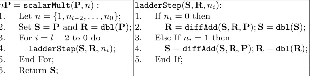
the Algorithms scalarMult and ladderStep are given in the Table 2. Notice that, Algorithm
ladderStep uses “If” condition, but in our implementated code of the ladder step we do not use
any branching instruction.
We start Algorithm scalarMult with two points S = P and R = 2P = dbl(P). Let at i-th iteration, the inputs be the points S =mP and R = (m+ 1)P. Then if ni = 0, the ladderStep outputs the points S= 2mP and R= (2m+ 1)P. On the other hand, if ni = 1, the ladderStep computes the pointsS= (2m+ 1)Pand R= 2(m+ 1)P.
nP=scalarMult(P, n) : ladderStep(S,R, ni): 1. Letn={1, nl−2, . . . , n0}; 1. Ifni= 0 then
2. SetS=PandR=dbl(P); 2. R=diffAdd(S,R,P);S=dbl(S); 3. Fori=l−2 to 0 do 3. Else Ifni= 1 then
4. ladderStep(S,R, ni); 4. S=diffAdd(S,R,P);R=dbl(R); 5. End For; 5. End If;
6. ReturnS;
Table 2.Scalar Multiplication and Ladder Step
2.2 Binary Kummer Line and the associated Elliptic Curve
Letb∈k and b6= 0. Let Eb be an elliptic curve defined over fieldkby Equation 3
Eb :Y2+XY =X3+b4. (3)
We can map a point of Kummer Line to elliptic curve by the mappingπ:BKL(1,b)→Eb/{±1} [13] which is defined as
π(P= (x, z)) =
(bz,·, x), ifx6= 0
∞, ifx= 0 (4)
Putting X = bzx in Equation 3, we can compute the Y-coordinate upto to the sign. We can also move back to Kummer line BKL(1,b) from Eb/{±1} using the inverse mapping π−1 as defined by Equation 5. LetP = (X,·, Z)∈Eb be a point ofEb then
π−1(P) =
(bZ,·, X), ifX 6= 0
(0,1), ifX= 0 (5)
2.3 Equivalence between BKL(1,b) and Eb
LetBKL(1,b)be a Kummer line on the binary fieldkandEbbe the associated elliptic curve as defined by Equation 3. Let P be a point on Kummer line BKL(1,b). Also consider the point T2 = (0, b2)
which is a point of order two onEb. Asπ(P) is a point onEb,π(P) +T2 is also a point onEb. Now we extend the mapping π to ˆπ as given by Equation 6
ˆ
π(P) =π(P) +T2. (6)
The inverse mapping of ˆπ is defined as
ˆ
π−1(P) =π(P+T2), (7)
whereP is a point onEb. Let P= (x, z) be a point on the Kummer line such that it is not a point of order 2 or identity, then Equation 8 holds.
2ˆπ(P) = ˆπ(dbl(P)). (8)
LetP1 and P2 be any two points on Eb such thatP16=±P2 and neither of them is point at infinity
nor of order 2. Then Equation 9 hold.
ˆ
π dbl(ˆπ−1(Pi))
= 2Pi, i= 1,2 ˆ
π diffAdd(ˆπ−1(P1),πˆ−1(P2),ˆπ−1(P1−P2))
=P1+P2
(9)
Notice that 2ˆπ(P) = 2 (π(P) +T2) = 2π(P). The proofs of Equations 8 and 9 are trivial, but
the expressions grow very fast and hard to compute manually. Therefore, we used GP/PARI [29] script to verify them symbolically and made available along with the software. Equations 8 and 9 are important as they forms the consistency between the scalar multiplications of binary Kummer Line BKL(1,b) and elliptic curve Eb. Let P ∈ BKL(1,b). Then we have ˆπ(nP) = nˆπ(P). Again, we
have that ˆπ(nP) = π(nP) +T2 and nˆπ(P) = n(π(P) +T2) =nπ(P) +n (mod 2)T2. Therefore,
ˆ
π(nP) =nˆπ(P) can be rewritten as
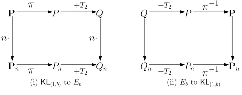
π(nP) =nπ(P) + (1 +n(mod 2))T2
which is pictorially shown in Figure 1. The equivalence of scalar multiplication on Kummer line
P
Pn
P
Pn
Q
Qn π +T2
π +T2
n· n·
Q P P
Pn
Pn
Qn +T
2
+T2 π−1
π−1 (i)KL(1,b)toEb (ii)EbtoKL(1,b)
Fig. 1.Consistency of scalar multiplications betweenBKL(1,b) andEb
3 Binary Edwards Curve
In this section, we give a brief description of binary Edward curve to make the paper self-contained. Let k be a field of characteristics 2. Let d ∈ kr{0}. We define binary Edwards curve [8, 5] by
Equation 10.
BEd:d(x+x2+y+y2) = (x+x2)(y+y2) (10)
The neutral element is the point (0,0). The point (1,1) has order 2. The Edwards curve BEd is birationally equivalent to the ordinary curveEd of Equation 11.
Ed:X2+XY =X3+ (d2+d)X+d8. (11)
The mapping from BEdtoEd is given by Equation 12.
φ: (x, y)7→(X, Y)
X= d
3(x+y)
xy+d(x+y) (12)
Y =d3
x
xy+d(x+y) +d+ 1
[8, 5] suggests the use ofW Z-coordinate system, whereW =X+Y, which provides the minimum operation count for the ladder step of Montgomery like scalar multiplication on binary Edwards curve. Let P, Q ∈ BEd such that P = (w2, z2), Q = (w3, z3) and P −Q = (w1,1) are given. We
compute 2P = (w3, z3) and P +Q = (w4, z4) using mixed differential and doubling operation as
given in Table 3. We refer [8, 5] for further details of binary Edwards curve.
c=w2(w2+z2); w4=c4; z4=d(z22)2+w4;
v=cw3(w3+z3);z5=v+d(z2z3)2;w5=v+z5w1;
Table 3.Mixed differential and doubling of binary Edwards Curve
4 Kummer Line over Field F2251
Let q be an integer and k =F2q be a finite field of characteristics 2 with 2q elements. We choose
Kummer line BKL(1,b) such that b 6= 0 and b ∈ F2q and then we check whether the associated
elliptic curveEb is one with all the required security criteria like curve and the twist of it have near prime orders, have large prime subgroups, resistance against pairing attacks and others which we discuss in details for the proposed Kummer line later. In this work, we target 128-bit security and we choose fieldF2251 =F2[t]/(t251+t7+t4+t2+ 1) as the binary Edwards curveBEd251[8, 5] and the binary Weierstrass curveCURVE2251[28]. For BEd251,d=t57+t54+t44+ 1.
1. Order of the curve is 4p1 where p1 = 2249 −δ1 and δ1 = 16097863035246445898362306\
660609333279. Therefore, the curve order is near prime [5] with cofactor h= 4.
2. Order of the twist curve is 2p2 where p2 = 2250 +δ2 and δ2 = 3219572607049289179672\
4613321218666559. Similarly, the twist curve order is near prime [5] with cofactor hT = 2. 3. The largest prime subgroup has order p1 and of size 249-bit. Therefore the curve provides
approximately 124.5-bit security against discrete logarithms problem.
4. Avoiding subfields: The j-invariant 1/b4 is a primitive element of the field F2251. 5. The discriminant of the curve is ∆ = (2251+ 1−4p1)−4·2251
which is 1 (mod 4) and a square-free term. The discriminant is also divisible by the large prime ∆/(−7·31·599·2207). 6. The multiplicative order of 2251 (mod p1) and 2251 (mod p2) are very large and they are
respectively λ = (p1 −1)/2 and λT = (p2 −1)/6. Therefore, the curve is resistant against
pairing attacks.
7. Similar to the BEd251, it is also resistant against GHS attack as the degree of the extension field is 251 which is a prime [5, 21].
From hereon,BKL251 denotes theBKL(1,b) withb=t13+t9+t8+t7+t2+t+ 1 over the finite field
F2251. The Kummer line BKL251 also has a small base point (t3+t2,1), where other two curves have long base points. Table 4 lists the comparative study of (estimates of) the sizes of the various parameters of the associated elliptic curve of the proposed Kummer lines BKL251 with respect to theBEd251and theCURVE2251.
(lgp1,lgp2) (h, hT) (λ, λT) lg(−∆) Base point BEd251[8, 5] (249,250) (4,2) (p1−1
2 ,
p2−1
2 ) 252
-CURVE2251[28] (249,250) (4,2) (p1−1 2 ,
p2−1
6 ) 253 (α1, γ1) BKL251 (this work) (249,250) (4,2) (p1−1
2 ,
p2−1
6 ) 253 (α2,1)
α1 = 0x6AD0278D8686F4BA4250B2DE565F0A373AA54D9A154ABEF ACB90\
DC03501D57C,
γ1 = 0x50B1D29DAD5616363249F477B05A1592BA16045BE1A9F218180C5150\
ABE8573, α2 = 0xC.
Table 4.Comparison ofBKL251 against BEd251andCURVE2251
4.1 Set of Scalars
In this work, the allowed scalars are of length 251 bits and have the from
2250+ 4· {0,1,2, . . . ,2248−1}.
We call this scalars asclamped scalar following the terminology of [17]. Use of clamped scalars ensures two things:
2. Constant time scalar multiplication. The most traditional way to achieve constant time scalar multiplication is the use of Montgomery ladder. In Montgomery ladder, the ladder step iterates (l−1) times where l is the bit-length of the scalar. This implies that the constant time is relative to the length of scalar. By clamping, we ensure the use of constant number of iterations in the ladder step irrespective of the choice of the scalar. For BKL251, we always need 250 differential additions and 250 doubling.
Generation of Clamped Scalars One can create a clamped scalar from a 32-byte random binary string. First, clear the least significant two bits (that is, set zero to bit number 0 and 1 of 0-th byte). Second, clear the most significant 5 bits (that is, set 0 to bit number 7, 6, 4, 5, 4, and 3 of 31-st byte). Lastly set the 3-rd least significant bit of 31-st byte to 1 (that is, set 1 to bit number 2 of 31-st byte).
5 Field Arithmetic
Efficient field arithmetic is extremely necessary to have efficient scalar multiplication. There are many efficient algorithms which are available for binary field arithmetic, but we focus only on the finite fieldF2251 =F2[t]/(t251+t7+t4+t2+ 1) wheref(t) =t251+r(t) is a irreducible polynomial withr(t) = (t7+t4+t2+ 1). Each element ofu∈F2251 can be represented as a polynomial of the form
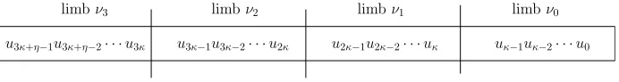
u=u250t250+u249t249+· · ·+u1t+u0, where eachui ∈F2,∀06i6250.
Element u can also be represented as binary vector of the form (u250, u249, . . . , u1, u0). We can
divide this vector intoνsmall vectors and we call this small vectors as limbs. Assume that the least significantν−1 limbs have lengthκand then length the most significant limb isη = 251−κ·(ν−1) as given in Figure 2.
uκ−1uκ−2· · ·u0
u2κ−1u2κ−2· · ·uκ
u3κ−1u3κ−2· · ·u2κ
u3κ+η−1u3κ+η−2· · ·u3κ
limbν0
limbν1
limbν2
limbν3
Fig. 2.Field element representation
In our implementation, our main objective is to explore the instruction PCLMULQDQ of Intel Intrinsic [16]. Let x and y be two 128-bit registers as m128i. We representx as a vector (x0, x1)
where x0 is the least significant 64 bits and x1 is the most significant 64 bits. Similarly we also
represent the y as (y0, y1). The instruction PCLMULQDQ takes two m128i variables and an 8-bit
integer 0xij (0x stands for hexadecimal representation), where i, j ∈ {0,1}, as inputs. Let z be another m128iregister. The PCLMULQDQ outputs
z= (z0, z1) =PCLMULQDQ(x, y,0xij) =xi2yj,
where (z1kz0) is the result of the binary multiplication ofxi andyj,kdenotes string concatenation and2denotes multiplication onF2. Notice thatPCLMULQDQcan only multiply two binary elements
5.1 Notation
The following notions are used to explain the algorithms of field arithmetic which we have imple-mented in our software.
kconcatenation of binary strings,
`left shift by`bits,
`right shift by`bits, & bitwise AND,
⊕bitwise XOR,
2multiplication of two elements inF2[t] by PCLMULQDQ,
len(u) length of a binary string u,
lsb`(u) least significant `bits of a binary stringu, and deg(f) degree of the polynomial f.
5.2 Field Element Representation
Letθ=t64∈F2[t]. Each element u∈F2251 is represented as u(θ) as given below:
u(θ) =u0+u1θ+u2θ2+u3θ3,
where eachui is thei-th limb as shown in Figure 2. We callu(θ) has proper representation if each ui < θfor i= 0,1,2 and u3 < t59. In other words, len(ui) 664 fori= 0,1,2 and len(u3)659 as
len(ui) = deg(ui) + 1 where ui is a binary polynomial.
5.3 Reduction
Reduction is one of the most important algorithms of field arithmetic. Let u(t) ∈ F2[t] such that
deg(u) = 251 +i. Then we can write u = h(t)t251 +g(t) where h(t), g(t) ∈ F2[t]/f(t) such that
deg(h(t)) =iand deg(g(t))6250. Then we have
u(t) =h(t)t251+g(t) =r(t)h(t) +g(t) (modf(t)).
Let u(θ) = P3
i=0u0θi where deg(ui) < 127 for i = 0,1,2 and deg(u3) < 117. Now if for
any i = 0,1,2, deg(ui) > 63 and/or deg(u3) > 58 then u(θ) is not a proper one. Following the
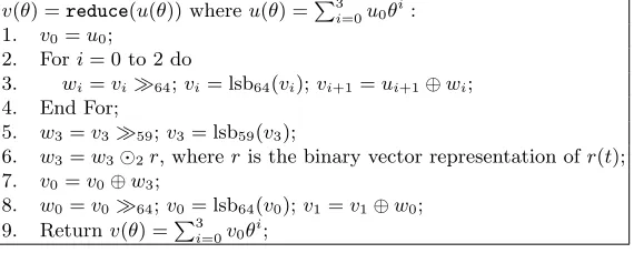
ideas of [4, 15, 3, 17], the reduction algorithmreduceis given in Table 5. Notice that the returned v(θ) is a proper one. After the For loop at line 4, len(vi) 6 64 for i = 0,1,2 and len(v3) 6
max{len(u3),len(w2)} 6max{118,127−64} = 118. After line 5, len(v3) 6 59 and len(w3) 6 59.
This implies thatw3 is a binary polynomial of maximum degree 58. Asr is a polynomial of degree
7, deg(w3) can be at most 65 after line 6 that is len(w3) 666. Then v0 can be of length 66 bits
after line 7 which is 2-bit greater than the allowed 64-bit. Line 8 takes care of this overflow fromv0.
As XOR do not increase the length of the input binary strings and len(v1)664 at the beginning
of line 8, then len(v1) is still at most 64 bits after line 8. This concludes that the outputv(θ) is the
v(θ) =reduce(u(θ)) whereu(θ) =P3i=0u0θi:
1. v0=u0;
2. Fori= 0 to 2 do
3. wi=vi64;vi= lsb64(vi);vi+1=ui+1⊕wi;
4. End For;
5. w3=v359;v3= lsb59(v3);
6. w3=w32r, whereris the binary vector representation ofr(t);
7. v0=v0⊕w3;
8. w0=v064;v0= lsb64(v0);v1=v1⊕w0;
9. Returnv(θ) =P3i=0v0θi;
Table 5.Algorithmreduce
5.4 Addition and Subtraction
Let u(θ) = P3
i=0u0θi and v(θ) =
P3
i=0v0θi be two elements of F2251 with proper representations. Let w(θ) = u(θ) +v(θ) ∈ F2251. Addition over binary field is very easy and only needs XOR operations. We compute addition algorithm addas wi =ui⊕vi for alli= 0,1,2,3 where w(θ) =
P3
i=0wiθi is also in proper representation. As binary addition operation is component-wise XOR,
it is not followed by thereducealgorithm.
On binary field, subtraction is the same as the addition as −1 = 2−1 = 1. Therefore, we do not define subtraction separately.
5.5 Multiplication by Small Constant
Let u(θ) =P3
i=0uiθi be an element of the field F2251. We would like to multiply u(θ) by a small constantc(let). By small constant, we mean thatc∈F2[t] and deg(c)663. This also implies that
c can be stored using only one limb. We compute the multiplication as u0(θ) = P3
i=0(c2 ui)θi and then applyreduceon u0(θ) to achieve proper representation. The Algorithm is summarized in Table 6.
v(θ) =constMult(u(θ), c) : 1. Fori= 0 to 3 do 2. u0i=ui2c; 3. End For;
4. v(θ) =reduce(u0(θ)) 5. Returnv(θ) =P3i=0v0θi;
Table 6.AlgorithmconstMult
5.6 Field Multiplication
Let u(θ) = P3
i=0u0θi and v(θ) =
P3
i=0v0θi be two elements with proper represntation to be
multiplied. Then the multiplication algorithm is given in the Table 7. The function polyMult of u(θ) andv(θ) computes a polynomial of degree 6 inθ. Let the polynomial bew(θ) =P6
applyexpandMfunction onw(θ) to achieve a polynomial of 8 limbs where each limb is of at most 64-bit. The steps of the AlgorithmexpandMare also given in the Table 7. Let the expanded polynomial be w(θ) =P7
i=0wiθi with len(wi) 664. Then we can derive Equation 14 from the output of the
functionexpandM (that is Equation 13) using the functionfold(w(θ)) as given below.
w(θ) =w7θ7+w6θ6+w5θ5+w4θ4+w3θ3+w2θ2+w1θ+w0 (13)
= (w7θ3+w6θ2+w5θ+w4)θ4+ (w3θ3+w2θ2+w1θ+w0)
= (w7θ3+w6θ2+w5θ+w4)t5t251+ (w3θ3+w2θ2+w1θ+w0)
= (w7θ3+w6θ2+w5θ+w4)rt5+ (w3θ3+w2θ2+w1θ+w0) [As f(t) =t251+r(t)]
= (w3+w7rt5)θ3+ (w2+w6rt5)θ2+ (w1+w5rt5)θ+ (w0+w4rt5) (14)
w(θ) =mult(u(θ), v(θ)) : w(θ) =expandM(w(θ)) : 1. w(θ) =polyMult(u(θ), v(θ)) 1. w7= 0;
2. w(θ) =expandM(w(θ)); 2. Fori= 0 to 6 do
3. w(θ) =fold(w(θ)); 3. wi+1=wi+1⊕(wi64);wi= lsb64(wi);
4. w(θ) =reduce(w(θ)) 4. End For;
5. Returnw(θ) =P3i=0wiθi; 5. Returnw(θ) =P7i=0wiθi;
Table 7.AlgorithmsmultandexpandM
Notice that theexpandMis absolutely necessary. AfterpolyMultat line 1 ofmult(u(θ), v(θ)), we havew(θ) =P6
i=0wiθi. In the absence ofexpandMfunction, consider the termswirt5 fori= 4,5,6. AfterpolyMult(u(θ), v(θ)),wiis a polynomial of degree at most 127. As deg(r) = 7, thenwirt5can be a polynomial of degree 126 + 7 + 5 = 138 which requires 139 bits to store. In our implementation, we use m128i whose capacity is 128-bit. Therefore, without expandM, there will be overflow.
Computation polyMult(u(θ), v(θ)). Letu(θ) andv(θ) be in proper representation with 4 limbs and let w(θ) = polyMult(u(θ), v(θ)). w(θ) is a polynomial of the form w(θ) = P6
i=0wiθi. The main objective of the function polyMult is the computation of the coefficients of w(θ) that is wi for i = 0,1, . . . ,6. We use PCLMULQDQ and XOR to compute the coefficients using a hybrid method of 2-2 Karatsuba [24] method and school-book method. The 2-2 Karatsuba method used in implementation is as given below:
w(θ) =polyMult(u(θ), v(θ))
=polyMult2(u1θ+u0, v1θ+v0) +polyMult2(u3θ+u2, v3θ+v2)θ4+
(polyMult2((u1⊕u3)θ+ (u0⊕u2),(v1⊕v3)θ+ (v0⊕v2)) +
(polyMult2(u1θ+u0, v1θ+v0) +polyMult2(u3θ+u2, v3θ+v2)))θ2
On the other hand, polyMult2is computed using school-book method as
polyMult2(u1θ+u0, v1θ+v0) = (u12v1)θ2+ + ((v12u0)⊕(v02u1))θ
(u02v0)
Each polyMult2 requires 4 PCLMULQDQ operations and 1 XORs. Consequently, polyMult requires
Unreduced Field Multiplication (multUnreduced). Letu(θ) andv(θ) be two elements ofF2251 with proper representation that isu(θ) =P3
i=0uiθi andv(θ) =P3i=0viθi. Letw(θ) is a polynomial of the formw(θ) =P6
i=0wiθi. We definemultUnreducedas
w(θ) =multUnreduced(u(θ), v(θ)),
where multUnreduced(u(θ), v(θ)) = polyMult(u(θ), v(θ)). multUnreduced(u(θ), v(θ)) is exactly the same as themullt without expandM,fold and reduce.
Field Addition of unreduced field elements (addReduce). Let u(θ) =P6
i=0uiθi and v(θ) =
P6
i=0viθi be two elements ofF2251 whereu(θ) andv(θ) are results ofmultUnreduceds asaddReduce is used on the outputs of twomultUnreducedin our implementation. As addition over binary field is simply the bit-wise XOR of the inputs, it does not increase the length and thus there is no issue of overflow. The details of the algorithm of addReduce is given in Table 8. On the XORed value, we applyexpandM,fold and reduceto attend a proper representation.
w(θ) =addReduce(u(θ), v(θ)) : 1. Fori= 0 to 6 do
2. wi=ui⊕vi; 3. End For;
4. w(θ) =expandM(w(θ)); 5. w(θ) =fold(w(θ)); 6. w(θ) =reduce(w(θ)); 7. Returnw(θ) =P3i=0wiθi;
Table 8.AlgorithmsaddReduce
5.7 Field Squaring
Field squaring is much less expensive in binary fields compared to prime fields as here squaring means relabeling the exponent of the input binary element. Letu(θ) =P3
i=0u0θi be the element to
be squared. The squaring algorithm is given in Table 9. ThepolySqfunction creates a polynomial w(θ) =P6
i=0wiθi fromu(θ) as given in Equation 15.
wi=
u2i/2, i= 0 (mod 2)
0, , i= 1 (mod 2) (15)
As a consequence, the expandS is also slightly different that expandM. In function expandS, if i= 0 (mod 2), then we divide the wi in to two parts and assign the least significant 64 bits to wi and the remaining most significant bits towi+1. If i= 1 (mod 2), we do nothing. The details of the
functionexpandSare also given in Table 9. On the output ofexpandS, we applyfold andreduce to compute the proper representation of the squared value.
w(θ) =sq(u(θ)) : w(θ) =expandS(w(θ)) : 1. w(θ) =polySq(u(θ), v(θ)) 1. Fori= 0,2,4,6 do
2. w(θ) =expandS(w); 2. wi+1= (wi64);wi= lsb64(wi);
3. w(θ) =fold(w); 3. End For;
4. w(θ) =reduce(w(θ)) 4. Returnw(θ) =P7i=0wiθi; 5. Returnw(θ) =P3i=0wiθi;
Table 9.AlgorithmssqandexpandS
5.8 Field Inverse
We compute Kummer Line scalar multiplication in projective coordinate system and receive an projective point (xn, zn) at the end of the iterations of ladder steps. Therefore, we compute the affine output asxn/znwhich requires one field inversion and one field multiplication. We compute field inversion asz−n1 =z2n251−2in constant time using 250 field squaring and 10 field multiplications following the sequence given in [5]. The multiplications produce the terms z3n, zn7, zn26−1, z2n12−1, zn224−1,zn225−1,zn250−1,z2n100−1,zn2125−1 and z2n250−1.
5.9 Conditional Swap
The ladderstep of Table 2 uses conditional swap based on the input bit from the scalar. But
to achieve constant time scalar multiplication, no use of branching instructions is prerequisite. Therefore, we perform the conditional swap without any branching instruction as given in Table 10. In Table 10, the algorithm condSwap uses branching instruction where condSwapConst performs the same job as the condSwapwithout any branching instruction. In computer, 0 is represented as a binary sting of all zeros and −1 is represented as a binary string of all ones in 2’s complement representation. Therefore, ifbis 0 thenw= 0 at the end of the line 2 of AlgorithmcondSwapConst else it is w = ui ⊕vi. As a consequence, if b = 0, there is no change of values in ui and vi as ui =ui⊕0 =ui and vi =vi⊕0 =vi. On the other hand, if b= 1, then ui and vi get swapped as ui =ui⊕w=ui⊕ui⊕vi =vi and vi=vi⊕w=vi⊕ui⊕vi=ui.
condSwap(u(θ), v(θ),b) condSwapConst(u(θ), v(θ),b) 1. If (b= 1) then 1. Fori= 0 to 4 do
2. Fori= 0 to 4 do 2. w=ui⊕vi;w=w&(−b); 3. w=ui;ui=vi;vi=w; 3. ui=ui⊕w;vi=vi⊕w; 4. End For; 4. End For;
5. End If;
Table 10.Algorithm Conditional Swap
6 Scalar Multiplication
6.1 Scalar Multiplication of BKL251
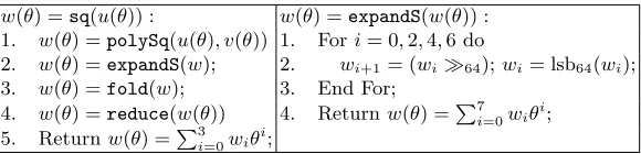
The algorithms for scalar multiplication BKLscalarMult and BKLscalarMultFB are given in Ta-ble 11. Algorithms BKLscalarMult is scalar multiplication algorithm when the base point is un-known from before hand and we call it variable-base scalar multiplication. On the other hand,FBof BKLscalarMultFBstands for fixed-base and, we pre-compute the pointdbl(P) and keep it in mem-ory. We alway consider that thez-coordinate of the input base point is 1 and the implementation is designed to take advantage of that. The total operation counts of ladder step ofBKLscalarMultis 5[M] + 5[S] + 1[C] where [M] denotes field multiplicationmult, [S] stands for field squaringsqand we denote multiplication by small constant by [C]. 1[C] refers the multiplication by Kummer Line pa-rameterb(line 25 ofBKLscalarMultand line 22 ofBKLscalarMultFB). In out implementation, the base point is a small one (t3+t2,1) which can be stored in one limb and consequently the field mul-tiplication in line 20 ofBKLscalarMultbecomes a multiplication by constant inBKLscalarMultFB (line 17). The total operation counts of ladder step ofBKLscalarMultFBbecomes 4[M] + 5[S] + 2[C].
BKLscalarMult(P, n) : BKLscalarMultFB(P,dbl(P), n) :
Input: Base Point = (x(θ),1) Input: Base Points = (x(θ),1, x2(θ), z2(θ))
n={1, nl−2, nl−3, . . . , n0} n={1, nl−2, nl−3, . . . , n0}
Output:xn(θ) Output:xn(θ)
1. sx(θ) =x(θ);sz(θ) = 1; 1. sx(θ) =x(θ);sz(θ) = 1; 2. t1(θ) =add(sx(θ)),sz(θ)); 2. rx(θ) =x2(θ);rz(θ) =z2(θ);
3. rx(θ) =sq(t1(θ)); 3. pb= 0;
4. rx(θ) =multConst(rx(θ), b); 4. Fori= (l−2) to 0 do 5. rz(θ) =sq(sx(θ)); 5. b= (pb⊕ni);
6. pb= 0; 6. condSwapConst(sx(θ),rx(θ),b); 7. Fori= (l−2) to 0 do 7. condSwapConst(sz(θ),rz(θ),b); 8. b= (pb⊕ni); 8. t1(θ) =add(sx(θ),sz(θ));
9. condSwapConst(sx(θ),rx(θ),b); 9. t2(θ) =add(rx(θ),rz(θ));
10. condSwapConst(sz(θ),rz(θ),b); 10. t3(θ) =mult(t1(θ), t2(θ));
11. t1(θ) =add(sx(θ),sz(θ)); 11. t3(θ) =sq(t3(θ));
12. t2(θ) =add(rx(θ),rz(θ)); 12. t4(θ) =multUnreduced(sx(θ),rz(θ));
13. t3(θ) =mult(t1(θ), t2(θ)); 13. t5(θ) =multUnreduced(sz(θ),rx(θ));
14. t3(θ) =sq(t3(θ)); 14. rz(θ) =addReduce(t4(θ), t5(θ));
15. t4(θ) =multUnreduced(sx(θ),rz(θ)); 15. rz(θ) =sq(rz(θ));
16. t5(θ) =multUnreduced(sz(θ),rx(θ)); 16. rx(θ) =add(t3(θ),rz(θ));
17. rz(θ) =addReduce(t4(θ), t5(θ)); 17. rz(θ) =multConst(rz(θ), x(θ));
18. rz(θ) =sq(rz(θ)); 18. sz(θ) =mult(sx(θ),sz(θ)); 19. rx(θ) =add(t3(θ),rz(θ)); 19. sz(θ) =sq(sz(θ));
20. rz(θ) =mult(rz(θ), x(θ)); 20. sx(θ) =sq(t1(θ));
21. sz(θ) =mult(sx(θ),sz(θ)); 21. sx(θ) =sq(sx(θ));
22. sz(θ) =sq(sz(θ)); 22. sx(θ) =multConst(sx(θ), b(θ)); 23. sx(θ) =sq(t1(θ)); 23. pb=ni;
24. sx(θ) =sq(sx(θ)); 24. End For;
25. sx(θ) =multConst(sx(θ), b(θ)); 25. condSwapConst(sx(θ),rx(θ), n0);
26. pb=ni; 26. condSwapConst(sz(θ),rz(θ), n0);
27. End For; 27. Return (sx(θ)/sz(θ)); 28. condSwapConst(sx(θ),rx(θ), n0);
29. condSwapConst(sz(θ),rz(θ), n0);
30. Return (sx(θ)/sz(θ));
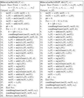
6.2 Scalar Multiplication of BEd251
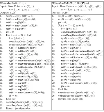
For scalar multiplication on binary Edwards curve BEd251, we use W Z-coordinate system which has minimu operation count per ladder step as suggested in [8, 5, 7]. The algorithms for scalar multiplicationBEdscalarMult and BEdscalarMultFBare given in the Table 12. Similar to binary Kummer line,BEdscalarMulttakes care of variable-base, whereBEdscalarMultFBis the algorithm for fixed-base scalar multiplication on binary Edwards curve. The operation counts of the ladder steps of BEdscalarMult is 5[M] + 4[S] + 2[C] where [C] is the multiplication by Edwards curve parameter d (lines 18 and 23 of BEdscalarMult and, lines 15 and 20 of BEdscalarMultFB). In W Z-coordinate system,W =X+Y. It is very hard to find a base point (x, y) on Edwards curve such that (x, y) is the generator of the largest prime subgroup andw=x+ybecomes small enough to be stored in a limb. Even if we try to make x small, y becomes a random element of the field which satisfies the Equation 10, that isy becomes the roots of the quadratic Equation 16
1 + d
x+x2
y2+
1 + d
x+x2
y+d= 0. (16)
Similar thing happens if we try to control the size ofy. In our experiment we could not find such a point and it seems only way is to check all the points of BEd251 by brute-forced method1. As a result, the operation counts in ladder step of BEdscalarMultFB remains the same as that of BEdscalarMult, that is 5[M] + 4[S] + 2[C].
7 Implementations and Timings
We have implemented the softwares using the Intel intrinsic instructions applicable to m128i. All the modules of the field arithmetics and the ladder step are written in assembly language to achieve the most optimized implementation. The 64×64 bit binary field multiplications are done using pclmulqdq instruction. We compute 128-bit bit-wise XOR and AND operations using instructionspxor andpand respectively. For byte-wise and bit-wise right-shift, we use psrldqand
psrlq. We implement the scalar multiplication function with clamped scalars and Montgomery
ladder algorithm with constant-time conditional swap algorithm and constant-time field inverse operation. Consequently, our code achieves constant time.
We use reducealgorithm with mult, sq,multConst and addReduce. In case of function mult and sq, the size of the limbs are at most 76 bits after fold operations. Therefore, thew3 of line 5
of Algorithm reduce(Table 5) will be 17 bits at most and in turnw3 becomes 24-bit after line 6.
Therefore, there will be no overflow from v0 of line 7 of Table 5. Similar situation will happen for
theaddReduce.
In case ofmultConstin scalar multiplicationsBKLscalarMultandBKLscalarMultFB, the max-imum length of the constant is the length of the Kummer line parameter b which is 14-bit (where the base point is of 4 bits). Therefore, the maximum possible length ofu03 after line 3 of Algorithm multConstis 72-bit. During reduceofmultConst,w3 of line 7 of Table 5 becomes 20-bit long and
in turn there will be no overflow from v0.
In case ofmultConstin scalar multiplicationsBEdscalarMultandBEdscalarMultFB, the max-imum length of the constant is curve parameter dwhich is of degree 57. Therefore, the maximum
1
BEdscalarMultKL(P, n) : BEdscalarMultFB(P,dbl(P), n) :
Input: Base Point = (w(θ),1) Input: Base Points = (w(θ),1, w2(θ), z2(θ))
n={1, nl−2, nl−3, . . . , n0} n={1, nl−2, nl−3, . . . , n0}
Output:xn(θ) Output:xn(θ)
1. sw(θ) =w(θ);sz(θ) = 1; 1. sw(θ) =w(θ);sz(θ) = 1; 2. t1(θ) =add(sw(θ)),sz(θ)); 2. rw(θ) =w2(θ);sz(θ) =z2(θ);
3. t2(θ) =mult(sw(θ), t1(θ)); 3. pb= 0;
4. rw(θ) =sq(t2(θ)); 4. Fori= (l−2) to 0 do
5. rz(θ) =add(rw(θ), d(θ)); 5. b= (pb⊕ni);
6. pb= 0; 6. condSwapConst(sw(θ),rw(θ),b); 7. Fori= (l−2) to 0 do 7. condSwapConst(sz(θ),rz(θ),b); 8. b= (pb⊕ni); 8. t2(θ) =add(sw(θ),sz(θ));
9. condSwapConst(sw(θ),rw(θ),b); 9. t2(θ) =mult(t2(θ),sw(θ));
10. condSwapConst(sz(θ),rz(θ),b); 10. t3(θ) =add(rw(θ),rz(θ));
11. t2(θ) =add(sw(θ),sz(θ)); 11. t3(θ) =mult(t3(θ),rw(θ));
12. t2(θ) =mult(t2(θ),sw(θ)); 12. t3(θ) =mult(t2(θ), t3(θ));
13. t3(θ) =add(rw(θ),rz(θ)); 13. t4(θ) =mult(sz(θ),rz(θ));
14. t3(θ) =mult(t3(θ),rw(θ)); 14. t4(θ) =sq(t4(θ));
15. t3(θ) =mult(t2(θ), t3(θ)); 15. t4(θ) =multConst(t4(θ), d);
16. t4(θ) =mult(sz(θ),rz(θ)); 16. t4(θ) =add(t3(θ), t4(θ));
17. t4(θ) =sq(t4(θ)); 17. sw(θ) =sq(t2(θ));
18. t4(θ) =multConst(t4(θ), d); 18. sz(θ) =sq(sz(θ));
19. t4(θ) =add(t3(θ), t4(θ)); 19. sz(θ) =sq(sz(θ));
20. sw(θ) =sq(t2(θ)); 20. sz(θ) =multConst(sz(θ), d);
21. sz(θ) =sq(sz(θ)); 21. sz(θ) =add(sz(θ),sw(θ)); 22. sz(θ) =sq(sz(θ)); 22. rw(θ) =mult(t4(θ), w(θ));
23. sz(θ) =multConst(sz(θ), d); 23. rw(θ) =add(rw(θ), t3(θ));
24. sz(θ) =add(sz(θ),sw(θ)); 24. rz(θ) =t4(θ);
25. rw(θ) =mult(t4(θ), w(θ)); 25. pb=ni;
26. rw(θ) =add(rw(θ), t3(θ)); 26. End For;
27. rz(θ) =t4(θ); 27. condSwapConst(sw(θ),rw(θ), n0);
28. pb=ni; 28. condSwapConst(sz(θ),rz(θ), n0);
29. End For; 29. Return (sw(θ)/sz(θ)); 30. condSwapConst(sw(θ),rw(θ), n0);
31. condSwapConst(sz(θ),rz(θ), n0);
32. Return (sw(θ)/sz(θ));
Table 12.AlgorithmBEdscalarMultandBEdscalarMultFB
possible length of u03 after line 3 of Algorithm multConst is 116-bit. DuringreduceofmultConst, w3 of line 7 of Table 5 can be at most 64-bit long and thus there will also be no overflow from v0.
As there will be no overflow from v0 after line 7 of reduce in all possible cases of mult, sq,
multConst and addReduce in context ofBKL251 andBEd251, we further optimize the field
arith-metic by removing the line 8 of reducein Table 5 during implementation.
In the modules of field multiplications and squaring, a significant amount of time is taken by the attempt of achieving the proper representation. In other words, the operations expandM/expandS,
fold and reduce, in total, take a considerable amount of time compared to polyMult/polySq.
Timing experiments were carried out on a single core of three platforms and their setups are listed in Table 13. OS of the computer with Sandy Bridge processor is 64-bit Ubuntu 16.04 and the code was compiled using GCC version 9.2.1. On the other hand, the OS of the computers with Haswell and Skylake processors is 64-bit Ubuntu 14.04 with GCC version 7.3.0.
Processor Processor Ubuntu GCC Version
Architecture Make 64-bit
Sandy Bridge IntelrXeonrCPU E5-1620 v4 @ 3.50GHz 16.04 9.2.1 Haswell Intel Core™i7-4790 4-core CPU @ 3.60 Ghz 14.04 7.3.0 Skylake Intel Core™i7-6500U 2-core CPU @ 2.50GHz 14.04 7.3.0
Table 13.Experimental Setup
During timing measurements, turbo boost and hyperthreading were turned off. An initial cache warming was done with 25,000 iterations and then the median of 1,00,000 iterations was recorded. The Time Stamp Counter (TSC) was read from the CPU to RAX and RDX registers by RDTSC instruction. The timings are listed in the Table 14.
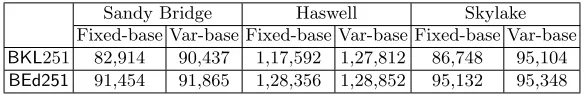
In Sandy Bridge,BKL251 is faster thanBEd251by 9.33% and 1.55% for fixed-base and variable-base scalar multiplications respectively. In Haswell architecture, we found thatBKL251 is faster than BEd251by 8.36% and 0.80% for fixed-base and variable-base scalar multiplications respectively. We get the similar results for Skylake architecture where the speedups for fixed-base and variable-base scalar multiplication are 8.81% and 0.25% respectively.
Sandy Bridge Haswell Skylake Fixed-base Var-base Fixed-base Var-base Fixed-base Var-base
BKL251 82,914 90,437 1,17,592 1,27,812 86,748 95,104
BEd251 91,454 91,865 1,28,356 1,28,852 95,132 95,348
Table 14.Timings of Scalar Multiplications ofBKL251 andBEd251in clock cycles (clk)
Diffie-Hellman Key Exchange.In two-party Diffie-Hellman key exchange [11] protocol, each party has to compute two scalar multiplication: one fixed-base and one variable-base. Ignoring the communication time, the total computation time required by each party is the sum of the computation time of both the scalar multiplication. The results are given in Table 15. In Sandy Bridge, Haswell and Skylake platforms, Diffie-Hellman key exchange which usesBKL251 are 5.43%, 4.58% and 4.52% faster than Diffie-Hellman key exchange withBEd251respectively.
Sandy Bridge Haswell Skylake
BKL251 1,73,351 2,45,404 1,81,852
BEd251 1,83,319 2,57,208 1,90,480
8 Conclusion
This work exhibits that Binary Kummer line based scalar multiplication offers competitive perfor-mance compared to existing proposal like BEd251 and CURVE2251 over finite field of character-istics 2 using PCLMULQDQ. Previous implementations of BEd251and CURVE2251 focuses on batch implementation using bitslicing technique. This work presents the first ever implementation of the proposedBKL251 andBEd251using the instructionPCLMULQDQ (best to our knowledge). From the experimental results, we conclude that BKL251 is approximately 9% and 1% faster than BEd251 for fixed-base and variable-base scalar multiplication respectively.
References
1. D. F. Aranha, 2019. Personal Communication.
2. D. F. Aranha. Relic-toolkit, 2019. https://github.com/relic-toolkit.
3. R. M. Avanzi, H. Cohen, C. Doche, G. Frey, T. Lange, K. Nguyen, and F. Vercauteren.Handbook of Elliptic and Hyperelliptic Curve Cryptography. Chapman & HallCRC, 1st edition, 2006.
4. D. J. Bernstein. Curve25519: New diffie-hellman speed records. InPublic Key Cryptography – PKC, volume 3958 ofLNCS, pages 207–228. Springer, 2006.
5. D. J. Bernstein. Batch binary edwards. InAdvances in Cryptology - CRYPTO, volume 5677 of LNCS, pages 317–336. Springer, 2009.
6. D. J. Bernstein. Batch binary edwards, 2017. https://binary.cr.yp.to/edwards.html.
7. D. J. Bernstein and T. Lange. Explicit-formulas database, 2019. https://www.hyperelliptic.org/EFD/. 8. D. J. Bernstein, T. Lange, and R. R. Farashahi. Binary edwards curves. InCryptographic Hardware and Embedded
Systems - CHES, volume 5154 ofLNCS, pages 244–265, 2008.
9. B. B. Brumley, S. ul Hassan, A. Shaindlin, N. Tuveri, and Kide Vuoj¨arvi. Batch binary weierstrass. InAdvances in Cryptology - LATINCRYPT, volume 11774 ofLNCS, pages 364–384. Springer, 2019.
10. C. Costello and P. Longa. Four(Q): Four-dimensional decompositions on aQ-curve over the Mersenne prime. In Advances in Cryptology - ASIACRYPT Part I, volume 9452 ofLNCS, pages 214–235. Springer, 2015.
11. W. Diffie and M. Hellman. New directions in cryptography.IEEE Transactions of Information Theory, 22(6):644– 654, 1976.
12. P. Gaudry, 2019. Personal Communication.
13. P. Gaudry and D. Lubicz. The arithmetic of characteristic 2 kummer surfaces and of elliptic kummer lines.Finite Fields and Their Applications, 15(2):246–260, 2009.
14. P. Gaudry and E. Thom´e. The mpfq library and implementing curve-based key exchanges. SPEED: Software Performance Enhancement for Encryption and Decryption, pages 49–64, 06 2007.
15. D. Hankerson, A. J. Menezes, and S. Vanstone. Guide to Elliptic Curve Cryptography. Springer Publishing Company, Incorporated, 1st edition, 2010.
16. Intel. Intel intrinsics guide, 2019. https://software.intel.com/sites/landingpage/IntrinsicsGuide/\#. 17. S. Karati and P. Sarkar. Kummer for genus one over prime-order fields. Journal of Cryptology, pages 1–38, 2019.
https://doi.org/10.1007/s00145-019-09320-4.
18. N. Koblitz. Elliptic curve cryptosystems. Math. Comp., 48(177):203–209, 1987. 19. Neal Koblitz. Hyperelliptic cryptosystems. Journal of Cryptology, 1(3):139–150, 1989.
20. C. H. Lim and P. J. Lee. A key recovery attack on discrete log-based schemes using a prime order subgroup. In Advances in Cryptology - CRYPTO, volume 1294 ofLNCS, pages 249–263. Springer, 1997.
21. A. Menezes and M. Qu. Analysis of the weil descent attack of gaudry, hess and smart. InTopics in Cryptology – CT-RSA, volume 2020 ofLNCS, pages 308–318. Springer, 2001.
22. V. S. Miller. Use of elliptic curves in cryptography. InAdvances in Cryptology - CRYPTO, LNCS, pages 417–426. Springer, 1985.
23. P. L. Montgomery. Speeding the pollard and elliptic curve methods of factorization.Mathematics of Computation, 48(177):243ˆa243, 1987.
24. P. L. Montgomery. Five, six, and seven-term karatsuba-like formulae. IEEE Trans. Computers, 54(3):362–369, 2005.
26. NIST. Fips pub 186-4: Digital signature standard (dss), 2013. https://nvlpubs.nist.gov/nistpubs/FIPS/ NIST.FIPS.186-4.pdf.
27. J. Renes and B. Smith. qDSA: Small and secure digital signatures with curve-based Diffie-Hellman key pairs. In Advances in Cryptology - ASIACRYPT, volume 10625 ofLNCS, pages 273–302. Springer, 2017.
28. J. Taverne, A. Faz-Hern´andez, D. F. Aranha, F. Rodr´ıguez-Henr´ıquez, D. Hankerson, and J. L´opez Hernandez. Speeding scalar multiplication over binary elliptic curves using the new carry-less multiplication instruction. J. Cryptographic Engineering, 1(3):187–199, 2011.