Actively Secure OT-Extension from
q
-ary Linear Codes
?Ignacio Cascudo , Ren´e Bødker Christensen , and Jaron Skovsted Gundersen
Department of Mathematical Sciences, Aalborg University
{ignacio,rene,jaron}@math.aau.dk
Abstract. We consider recent constructions of 1-out-of-NOT-extension from Kolesnikov and Kumaresan (CRYPTO 2013) and from Orr`u et al. (CT-RSA 2017), based on binary error-correcting codes. We generalize
their constructions such that q-ary codes can be used for any prime powerq. This allows to reduce the number of base 1-out-of-2 OT’s that are needed to instantiate the construction for any value ofN, at the cost of increasing the complexity of the remaining part of the protocol. We analyze these trade-offs in some concrete cases.
1
Introduction
AK-out-of-N oblivious transfer, or KN
-OT, is a cryptographic primitive that allows a sender to inputN messages and a receiver to learn exactly Kof these with neither the receiver revealing which messages he has chosen to learn nor the sender revealing the other N−K input messages. This is a fundamental cryptographic primitive in the area of secure multiparty computation, and in fact [9] showed that any protocol for secure multiparty computation can be implemented if the OT functionality is available. However, the results in [6] indicate that OT is very likely to require a public key cryptosystem, and therefore implementing OT is relatively expensive. Unfortunately, well-known protocols such as Yao’s garbled circuits [14] and the GMW-compiler [5] rely on using a large number of independent instances of OT. It is therefore of interest to reduce the number of OT’s used in a protocol in an attempt to reduce the overall cost. This can be done using what is called OT-extensions, where a large number of OT’s are simulated by a much smaller number of base OT’s together with the use of cheaper symmetric crypto primitives, such as pseudorandom generators.
Beaver showed in [1] that OT-extension is indeed possible, but it was not before 2003 that an efficient 21
-OT-extension protocol was presented by Ishai et al. in [7]. In addition, while this protocol had security against passive adversaries, subsequent work has shown that active security can be achieved at a small additional cost [8].
?The final authenticated publication is available online at https://doi.org/10.1007/
In [10], Kolesnikov and Kumaresan noticed that Ishai et al. were in essence relying on the fact that the receiver encodes its input as a codeword in a repetition code, and therefore one can generalize their idea by using other codes, such as the Walsh-Hadamard code, which not only obtains efficiency improvements for
2 1
-OT-extension, but also allows to generalize the protocol into passively secure
N
1
-OT-extension. In such an extension protocol the base OT’s are 21-OT’s, but the output consist of a number of N1
-OT’s. In more recent work, Orr`u et al. [12] and Patra et al. [13] transformed the protocol by [10] into an actively secure N1
-OT-extension protocol by adding a “consistency check” which is basically a zero-knowledge proof that the receiver is indeed using codewords of the designated code to encode his selections. As shown in [12,13], 1-out-of-N
oblivious transfer has a direct application to the problem of private set inclusion and, via this connection, to the problem of private set intersection. In fact this application requires only a randomized version of N1-OT, where the sender does not have input messages, but these are generated by the functionality and can be accessed on demand by the sender. The structure of the aforementioned OT extension protocols is especially well suited for this application, since such a randomized functionality is essentially implemented by the same protocol without the last step, where the sender would send its masked inputs to the receiver.
The aforementioned papers on N1-OT-extension relied on the use of binary linear codes, and the concrete parameters of the resulting construction, the number of OT’s and the value of N, are given respectively by the length and size of the binary linear code being used. Furthermore, the construction requires that the minimum distance of the code is at least the desired security parameter. Well-known bounds on linear codes, such as the Plotkin, Griesmer or Hamming bounds [11], provide lower bounds for the length of a code with certain size and minimum distance, and therefore these imply lower bounds on the number of base OT’s for the OT-extension protocol. In fact, even if we omit the requirement on the minimum distance, we can see that at least log2N base OT’s are needed for those extension protocols.
In this paper, we discuss the use ofq-ary linear codes, where q can be any power of a prime, as a way of reducing the number of required base OT’s in the 1-out-of-N OT-extension constructions mentioned above. We show that one can easily modify the protocol in [12] to work withq-ary codes, rather than just binary.1Given that all parameters of the code still have the same significance for
1 Update: In the published version of this work, we were unfortunately not aware of
the construction and, in particular,N is still the size (the number of codewords) of the code, we obtain a reduction in the number of base OT’s required: indeed, for given fixed valuesN andd, the minimal length among allq-ary linear codes of sizeN and minimum distancedbecomes smaller asqincreases. In particular one can show cases where the lower bound of log2N base OT’s can be improved even if we have relatively large minimum distance.
This improvement, however, comes at a cost: since we need to communicate elements of a larger field, the communication complexity of the OT-extension protocol (not counting the complexity of the base OT’s) increases. This increase is compensated to some extent by the fact that this communication complexity also depends on the number of base OT’s.
The concrete tradeoffs obtained by the use ofq-ary codes depend of course on
N and the security level. We show several examples comparing explicit results listed in [12] and the q-ary alternative achieving the same (or similar) N and security level. For example, for the largest value ofN considered in [12] we show that by using a linear code over the finite field of 8 elements, we need less than half of the base OT’s, while the communication complexity increases only by 33%.
Whenqis a power of two, we can show an improvement on the complexity of the consistency check that we use in the case of a general q. Namely, the consistency check in [12] works by asking the receiver, who has previously used the base OT’s to commit to both the codewords encoding his selections and some additional random codewords, to open sums of random subsets of these codewords. The natural way of generalizing this to a general prime powerqis to ask the receiver to open random linear combinations overFq of the codewords.
However, in case qis a power of two, we show that it is enough to open random linear combinations overF2, i.e., sums, just as in [12] (naturally, this extends to the case whereqis a power ofp, where it would be enough to open combinations overFp). The advantage of this generalization is of course that the verifier needs
to send less information to describe the linear combinations that it requests to open, and in addition less computation is required from the committer to open these combinations.
this consistency check by proving that rather than requesting the opening of uniformly random linear combinations of codewords, these combinations can be determined by a hash function randomly selected from an almost universal family of hash functions. This leads to asymptotical complexity gains, both in terms of communication and computation (since one can use linear time encodable almost universal hash functions which can in addition be described by short seeds), but in our case it also allows us to give a unified proof of security in both the case where the linear combinations for the consistency check are taken overFq and
when they are taken over the subfield.
The work is structured as follows. After the preliminaries in Section 2, we present our OT-extension protocol and prove its security in Section 3. In Sec-tion 4, we show that the communicaSec-tion cost can be reduced by performing the consistency checks over a subfield, and finally Section 5 contains a comparison with previous protocols.
2
Preliminaries
This section contains the basic definitions needed to present and analyse the protocol for OT-extension.
2.1 Notation
Throughout this paper, q will denote a prime power and Fq a finite field of q
elements. Every finite field has elements 0 and 1, and hence it will be natural to embed the set {0,1} in Fq.2 Bitstrings in {0,1}n and vectors fromFnq are
denoted in boldface. Thei-th coordinate of a vector or bitstringbis denotedbi.
For a bitstringb∈ {0,1}n, we will use the notation∆
bto denote the diagonal
matrix inFn×n
q with entries from the vectorb, i.e. the (i, i)-entry of∆bisbi. Note
that for vectors b,c∈Fn
q, the product c∆b equals the componentwise product
ofbandc.
2.2 Linear Codes
Since our protocol depends heavily on linear codes, we recall here the basics of this concept. First, a (not necessarily linear) code of lengthnover an alphabet
Qis a subset C ⊆Qn. AnF
q-linear codeC is anFq-linear subspace ofFnq. The
dimensionk of this subspace is called the dimension of the code, and therefore C is isomorphic to Fk
q. A linear map Fkq → C can be described by a matrix
G ∈Fk×n
q , which is called a generator matrix forC. Note that G acts on the
right, sow∈Fk
q is mapped to wG∈ C by the aforementioned linear map.
Forx∈Fn
q we define the support ofxto be the set indices wherexis nonzero,
and we denote this set by supp(x). Using this definition we can turn Fnq into
2 Of course, the elements of
a metric space. This is done by introducing the Hamming weight and distance. The Hamming weight ofxis defined aswH(x) =|supp(x)|, and this induces the
Hamming distancedH(x,y) =wH(x−y), wherey∈Fnq as well. The minimum
distancedof a linear codeCis defined to be
d= min{dH(c,c0)|c,c0∈ C,c6=c0},
and by the linearity of the code it can be shown that in fact
d= min{wH(c)|c∈ C \ {0}}.
Sincen,k, anddare fixed for a given linear codeC overFq, we often refer to it
as an [n, k, d]q-code.
It may be shown that ifx∈Fn
q is given byc+efor some codewordc∈ C
and an error vector e with wH(e) < d, it is possible to recover cfrom x and
supp(e). This process is called erasure decoding.
Another way to see erasure decoding is by considering punctured codes. For a set of indices E ⊆ {1,2, . . . , n} we denote the projection ofx∈Fn
q onto the
indices not inE byπE(x). For a codeC and a set of indicesE, we call πE(C) a
punctured code. Now consider the case where|E|< d, which implies the existence of a bijection betweenCandπE(C). This is the fact exploited in erasure decoding,
whereE is the set of indices where the errors occur. As in [2], we will use interleaved codes. IfC ⊆Fn
q is a linear code,C
sdenotes
the set ofs×n-matrices with entries inFq whose rows are codewords ofC. We
can also see such an s×n-matrix as a vector of length n with entries in the alphabet Fsq. Then we can see Cs as a non-linear3 code of length n over the
alphabetFs q.
Since the alphabetFs
q contains a zero element (the all zero vector), we can
define the notions of Hamming weight and Hamming distance in the space (Fs q)n.
We can then speak about the minimum distance ofCsand even thoughCsis
not a linear code, it is easy to see that the minimum distance of Cscoincides
with its minimum nonzero weight, and also with the minimum distance ofC.
2.3 Cryptographic Definitions
Consider a senderS and a receiverR participating in a cryptographic protocol. The sender holds vj,i ∈ {0,1}κ for j = 1,2, . . . , N and i = 1,2, . . . , m. For
eachi the receiver holds a choice integerwi ∈[1, N]. We let FNκ,m-OT denote the ideal functionality that, on inputsvj,ifrom S andwi from R, outputsvwi,ifor
i = 1,2, . . . , m to the receiver R. For ease of notation, we will let the sender inputN matrices of sizeκ×mwith entries in{0,1}, and the receiver a vector of length m, with entries in [1, N]. Hence, for the i’th OT the sender’s inputs are thei’th column of each matrix, and the receiver’s input is the i’th entry of the vector.
3 The code is linear overF
The protocol presented in Section 3 relies on two functions with certain security assumptions, the foundations of which we define in the following. For the first function let X be a probability distribution. The min-entropy of X is given by
H∞(X) =−log(max
x Pr[X =x]),
whereX is any random variable following the distributionX. IfH∞(X) =twe say thatX ist-min-entropy. This is used in the following definition.
Definition 1 (t-min-entropy strongly C-correlation robustness). Con-sider a linear code C ⊆ Fn
q, and let X be a distribution on {0,1}n with min-entropyt. Fix {ti∈Fqn|i= 1,2, . . . , m} from some probability distribution and letκbe a positive integer. An efficiently computable functionH:Fn
q → {0,1}κ is said to be t-min-entropy strongly C-correlation robust if
{H(ti+c∆b)|i= 1,2, . . . , m,c∈ C}
is computationally indistinguishable from the uniform distribution on{0,1}κm|C|
whenbis sampled according to the distribution X.
The second type of function we need is a pseudorandom generator.
Definition 2. A pseudorandom generator is a function PRG: {0,1}κ → Fm q such that the output ofPRGis computationally indistinguishable from the uniform distribution onFm
q .
IfA= [a1,a2, . . . ,an] is aκ×n-matrix with entries in{0,1}for some integern,
we use the notationPRG(A) = [PRG(a1),PRG(a2), . . . ,PRG(an)] where we see
PRG(ai) as columns of anm×nmatrix.
In addition to the usual concept of advantage, one can also consider the con-ditional advantage as it is done in [12]. LetAbe an event such that there existx0 andx1in the sample space of the two random variablesX0andX1, respectively, where Pr[Xi=xi|A]>0 fori= 0,1. Then we define the conditional advantage
of a distinguisherDgivenAas
Adv(D|A) =
Pr[D(X0) = 0|A]−Pr[D(X1) = 0|A] .
We end this section by presenting the following lemma, which allows us to bound the advantage by considering disjoint cases. The proof follows by the law of total probability and the triangle inequality.
Lemma 1. LetA1, A2, . . . , An be events as above. Additionally, assume that the events are disjoint. IfPni=1Pr[Ai] = 1, then
Adv(D)≤
n X
i=1
Adv(D |Ai) Pr[Ai]
3
Actively Secure OT-Extension
In this section we describe and analyse a generalization of the protocol described in [12] which uses OT-extensions to implement the functionalityFNκ,m-OTby using onlyn≤mbase OT’s, which are 1-out-of-2. Our OT-extension protocol is also using 1-out-of-2 base OT’s, but works withq-ary linear codes instead of binary. Our main result is summarized in the following theorem.
Theorem 1. Given security parametersκands, letCbe an[n, k, d]q linear code withk= logq(N)andd≥max{κ, s}. Additionally, letPRG:{0,1}κ→Fm+2s
q be
a pseudorandom generator and let H:Fn
q → {0,1}κ be a t-min-entropy strongly
C-correlation robust function for allt∈ {n−d+ 1, n−d+ 2, . . . , n}. If we have access to C, the functions PRG and H, and the functionality F2-OTκ,n , then the protocol in Figure 1 on page 8 implements the functionality FNκ,m-OT.
The protocol is computationally secure against an actively corrupt adversary.
3.1 The Protocol
We start by noticing that in our protocol R has inputs wi ∈ Fkq rather than
choice integers wi ∈[1, N]. However, the number of elements inFkq is qk =N,
and hencewi can for instance be theq-ary representation ofwi. In this way we
have a bijection between selection integers and input vectors.
Our protocol is, like the protocol in [12], very similar to the original protocol in [7]. The idea in this protocol is that we first do OT’s with the roles of the participants interchanged such that the sender learns some randomness chosen by the receiver. Afterwards,Rencodes his choice vectors using the linear codeCand hides the value with a one-time pad. He sends these toS, who will combine this information with the outputs of the OT functionality to obtain a set of vectors, only m of which R can compute; namely the ones corresponding to his input vectors. WhenS applies at-min-entropy stronglyC-correlation robust function
H to the set of vectors, he can use the outputs as one-time pads of his input strings. Like in [12] the protocol contains a consistency check to ensure thatR
acts honestly, or otherwise he will get caught with overwhelming probability. The full protocol is presented in Figure 1 on page 8.
In order to argue that the protocol is correct, we see that for each i, the senderS computes and sends the values yw,i for allw∈Fkq. Sincek= logq(N),
this yieldsN strings for each i∈ {1,2, . . . , m}. The receiver R obtains one of these because
H(qi−wiG∆b) =H(qi−ci∆b) =H(ti).
Furthermore, if both S and R act honestly, the consistency checks in phase 3 will always pass. This follows from the observation that
˜
T+ ˜W G∆b=M(T0+C∆b) =M Q.
3 In Section 4, we show if the protocol relies on a code overF
pr, it is enough to choose
M0
∈F2s×m
Hence, we note that if only passive security is needed in Protocol 1, we can omit phase 3 and sets= 0. The aforementioned steps are included to ensure that the receiver uses codewords in the matrixC. What a malicious receiver might gain by choosing rows which are not codewords is explained in [7, Sec. 4].
Protocol 1: OT-Extension
1. Initialization phase
(a) S chooses uniformly at randomb∈ {0,1}n.
(b) Rgenerates uniformly at random two seed matricesN0,N1∈ {0,1}κ×nand defines the matricesTi=PRG(Ni)∈F(m+2s)
×n
q fori= 0,1. (c) The participants call the functionality Fκ,n
2-OT, where S acts as the receiver
with input b, andRacts as the sender with inputs (N0, N1).S receivesN=
N0+ (N1−N0)∆b, and by usingPRG, he can computeT =T0+ (T1−T0)∆b. 2. Encoding phase
(a) LetW0
∈ Fk×m
q be the matrix which has wi as its columns.R generates a uniformly random matrixW00
∈Fk×2s
q , and defines the (m+ 2s)×k-matrix
W = [W0|W00]T.
(b) RsetsC=W G, and sendsU=C+T0−T1.
(c) S computesQ=T+U ∆b. This implies thatQ=T0+C∆b. 3. Consistency check
(a) Ssamples a uniformly random matrixM0
∈F2s×m
q and sends this toR.4 They both defineM= [M0
|I2s].
(b) Rcomputes the 2s×n-matrix ˜T =M T0and the 2s×k-matrix ˜W=M W and sends these matrices toS.
(c) S verifies thatM Q= ˜T+ ˜W G∆b. If this fails,Saborts the protocol. 4. Output phase
(a) Denote byqiandti, thei’th rows ofQandT0, respectively. Fori= 1,2, . . . , m
and for allw∈Fk
q,S computesyw,i=vw,i⊕H(qi−wG∆b) and sends these toR. Fori= 1,2, . . . , m,Rcan recovervwi,i=ywi,i⊕H(ti).
Fig. 1.This protocol implements the functionalityFκ,m
N-OThaving access toF
κ,n 2-OT. The
security of the protocol is controlled by the security parametersκands. The sender
S and the receiverR have agreed on a linear codeC ⊆Fn
q with generator matrixG of dimensionk= logq(N) and minimum distanced≥max{κ, s}. The protocol uses a pseudorandom generatorPRG:{0,1}κ
→Fm+2s
q and a functionH:Fnq → {0,1}κ, which ist-min-entropy stronglyC-correlation robust for allt∈ {n−d+ 1, n−d+ 2, . . . , n}.
R has m inputsw1,w2, . . . ,wm ∈ Fkq, which act as selection integers.S has inputs vw,i∈ {0,1}κ, indexed byi∈ {1,2, . . . , m}andw∈Fkq.
3.2 Proofs of Security
the proof against a malicious receiver in another way, where the structure, some strategies, and some arguments differ from the original proof.
Theorem 2. Protocol 1 is computationally secure against an actively corrupt sender.
Proof. To show this theorem we give a simulator, which simulates the view of the sender during the protocol. The view of S is ViewS = {N, U,T ,˜ W˜}. The
simulator SimS works as follows.
1. SimS receives b from S and defines a uniformly random matrix N, sets
T =PRG(N), and passesN back toS.
2. Then SimS samplesU uniformly at random and sends this toS. Additionally,
it computesQasS should.
3. In phase 3 the simulator receivesM0 fromS, and constructsM. The matrix ˜
W is sampled uniformly at random in F2qs×k, and using this, SimS sets
˜
T =M Q−W G∆˜ b. It sends ˜T and ˜W toS.
4. SimS receives yw,i from S and since SimS already knows Qand b, it can
recovervw,i=yw,i⊕H(qi−wG∆b) and pass these to the ideal functionality
FNκ,m-OT.
We now argue that the simulator produces values indistinguishable from ViewS.
The matrixN is distributed identically in the real and ideal world. Since both
T0 and T1 are outputs of a pseudorandom generator, the matrix T0−T1, and therefore alsoU, is computationally indistinguishable from a uniformly random matrix. In the real world, ˜W =M0(W0)T+ (W00)T is uniform sinceW00is chosen uniformly. The simulator SimS constructs ˜T such that the consistency check
will pass. This will always be the case in the real world, and hence S cannot distinguish between the real and ideal world. Additionally, we note that step 4 ensures that the receiver obtains the same output in both worlds. This shows security against an actively corrupt sender. ut
We now shift our attention to an actively corrupt receiver. This proof is not as straight forward as for the sender. The idea is to reduce the problem of breaking the security of the protocol to the problem of breaking the assumptions onH. Before delving into the proof itself, we will introduce some lemmata and notations that will aid in the proof. The focus of these will be the probability that certain events happen during the protocol. These events are based on situations that determine the simulator’s ability or inability to simulate the real world. Essentially, they are the event that R passes the consistency check, which we denote by PC; the event that R has introduced errors in too many positions, denoted byLS; and the event that the error positions from the consistency check line up with the errors in C, which we call ES. These will be defined more precisely below.
Inspired by the notation in the protocol, we define
˜
A corrupt receiver may deviate from the protocol and may send an erroneous ˜
W, which we denote by ˜W∗. Let
¯
C= ˜C−W˜∗G
and letE= supp( ¯C), where ¯C is interpreted inC2s. When writing ˜C, ¯C, and
E later in this section these are the definitions we are implicitly referring to.
Lemma 2. LetC, C, and M be as in Protocol 1. Further, let LS be the event that |E| ≥ s, and let ES be the event that for every C0 ∈ C2s there exists a
ˆ
C∈ Cm+2ssuch that supp( ˜C−C0) = supp(C−Cˆ). Then the probability that
neitherES norLS happen is at most q−s.
Proof. The matrixM0 in Protocol 1 is chosen uniformly at random, and hence
M can be interpreted as a member of a universal family of linear hashes. Thus, this lemma is a special case of [2, Theorem 1] when lettingm0=m+ 2s,s0=s, andt0= 0 where the primes denote the parameters in [2]. Additionally, note that our eventLS happens ifM C has distance at leastsfromC2s. ut
We will now bound the probability that an adversary is able to pass the consis-tency check, even if Ccontains errors.
Lemma 3. Let PCdenote the event that the consistency check passes. Then
Pr[PC]≤2−|E|.
Proof. In order to compute Pr[PC], we consider ¯C and ¯T = ˜T−T˜∗, where the∗ indicates that the matrix may not be constructed as described in the protocol. The eventPChappens ifM Q= ˜T∗+ ˜W∗G∆b. However, from the definition of
Q,M Q= ˜T+ ˜C∆b, implying thatPC happens if and only if
˜
T+ ˜C∆b= ˜T∗+ ˜W∗G∆b ⇐⇒ T¯=−C∆¯ b.
Now consider ¯T and ¯C in (Fnq)2s, meaning that the entries ¯Cj and ¯Tj are
elements in F2s
q . If the adversary chooses ¯Cj = 0 for some j ∈ {1,2, . . . , n}, it
must choose ¯Tj = 0 as well since the check would fail otherwise. If it chooses
¯
Cj 6= 0, it has two options. Either bet thatbj = 0 and set ¯Tj = 0 or bet that
bj = 1 and set ¯Tj =−C¯j. This means that for each entryj ∈E the adversary
has probability 12 of guessing the correct value of bj. For every entry j /∈ E,
each possible bj gives a consistent value since ¯Cj = ¯Tj = 0. By this and the
independence of the entries in b, it follows that the probability of the check passing is bounded by Pr[PC]≤2−|E|. ut
This immediately gives the following corollary.
Corollary 1. If LS denotes the same event as in Lemma 2, then
We now have the required results to prove the security of Protocol 1 against an actively corrupt receiver. The eventsPC,LS, andESfrom the previous lemmata and corollaries will also be used in the proof of the following theorem.
Theorem 3. Protocol 1 is computationally secure against an actively corrupt receiver.
Proof. As in the proof of Theorem 2, we construct a simulator SimR simulating
the view of the receiver, which is ViewR={M0,yw,i}. The simulator works as
follows.
1. SimR receivesN0 andN1 fromR.
2. The simulator receives U fromR and combines these with T0 =PRG(N0) and T1 =PRG(N1) to reconstruct the matrix C. Additionally, it samples uniformly at random an internal valueb. Using thisb, the simulator SimR
computesQ=T0+C∆b.
3. SimR samples a randomM0 like the sender would have done in the protocol
and sends this to R. In return, it receives ˜T∗ and ˜W∗, where the ∗ indi-cates that the vectors may not be computed according to the protocol. The simulator runs the consistency check and aborts if it fails.
4. Otherwise, it erasure decodes each row of C by lettingE be the erasures to obtainW0. If the decoding fails, it aborts. If the decoding succeeds, the simulator givesW0 as inputs to the ideal functionalityFNκ,m-OT, which returns the valuesvwi,ito SimR. It can now computeywi,i=vwi,i⊕H(qi−wiG∆b),
and choosesyw,i uniformly at random inFκq for allw6=wi.
The matrixM0 is uniformly distributed both in the real and ideal world. Hence, we only need to show that the outputyw,iproduced by the simulator is
indis-tinguishable from the output of the protocol.
LetZ be a distinguisher for distinguishing between a real world execution of the protocol and an ideal execution using the simulator. By Lemma 1 its advantage is bounded by
Adv(Z)≤Adv(Z |PC) + Adv(Z |PC,LS) Pr[PC|LS]
+ Adv(Z |PC,LS,ES) Pr[LS,ES] + Adv(Z |PC,LS,ES) Pr[PC], (2)
where we have omitted some probability factors since they are all at most 1. Notice thatywi,iis constructed identically in both worlds. The remaining yw,i
are uniformly distributed in the ideal world, but constructed as
yw,i=vw,i⊕H(qi−wG∆b) (3)
in the real world. Also notice that if the consistency check fails, the simulator aborts before constructing theyw,i. This is the same as in the real world, and the
Since the consistency check by the simulator is identical to the consistency check done by S, it follows that the probability for the consistency check to pass even if R might have sent inconsistent values is the same in both worlds. This means that Pr[PC|LS]≤2−sby Corollary 1. In a similar fashion, Lemma
2 implies that the penultimate term in (2) can be bounded above by q−s. In
summary, (2) can be rewritten as
Adv(Z)≤2−s+q−s+ Adv(Z |PC,LS,ES)2−|E|. (4)
To show that this is negligible inκands, assume the opposite; that is,Zhas non-negligible advantage. We then construct a distinguisherDbreaking the security assumptions onH.
The distinguisherD simulates the protocol with minor changes in order to produce its input to the challenger. After receiving the challenge it uses the output of Z to respond. There exist inputs and random choices for R and S, which maximize the advantage ofZ, and we can assume thatDhas fixed these in its simulation. This also means thatPC,LSandEShappen in the simulation since otherwise, Adv(Z) is negligible.
BecauseES happens, puncturingC in the positions in E gives a codeword inπE(Cm+2s). Further, the eventLS ensures that this corresponds to a unique
codeword inCm+2s. Hence,Dis able to erasure decode and fori= 1,2, . . . , m+
2s obtain ci = wiG+ei, where ci is the i’th row of C, wH(ei) < d, and
supp(ei)⊆E.
The following arguments use that no matter whichbthe challenger chooses, the distinguisherDknowsei∆b. This follows from the fact thatPChas happened
and thereforebj forj ∈E is known to the adversary, which is simulated by D.
Hence, the distinguisher is able to construct t0i=ti+ei∆b, where thebis the
vector eventually chosen by the challenger, and ti the i’th row ofT0. Letting
t=n− |E|, define the probability distributionX to be the uniform distribution onFn
2 under the condition that the indices inE are fixed to the corresponding entry ofb. By uniformity this distribution has min-entropyt. The distinguisher passesX and thet0ito the challenger. It receives backxw,ifor alli= 1,2, . . . , n
andw∈Fk
q and needs to distinguish them between being uniformly random and
being constructed as
xw,i=H(t0i+wG∆b), (5)
As in the protocol, letQ=T0+C∆b, wherebis again the vector chosen by the
challenger. Therefore, ifxw,i is constructed as in (5), we have that
xw,i=H(ti+ei∆b+wG∆b)
=H(qi−ci∆b+ei∆b+wG∆b)
=H(qi−(wi−w)G∆b).
The distinguisher will now construct and input toZ the following
ywi,i=vwi,i⊕H(t0i),
Sincet0i=ti+ei∆b=qi−wiG∆b, we have that ywi,iis identical to the value
computed in both the real and ideal worlds.
For the remainingwwe notice that if the challenger has chosenxw,iuniformly
at random, then the valuesyw,i are uniformly distributed as well. This is the
same as the simulator will produce in the ideal world. On the other hand, if xw,i=H(t0i+wG∆b), then we haveyw,i=vw,i⊕H(qi−w∆b). This is exactly
the same as produced during the protocol in the real world. Hence,Dcan feed the values yw,i to Z, which can distinguish between the real and ideal world,
and depending on the answer from Z,Dcan distinguish whether the xw,i are
uniformly distributed or are constructed asH(t0i+wG∆b). Hence, the advantage
ofDis the same as that ofZ under the restriction that PC,LS, andEShappen. This means that
Adv(D) = Adv(Z|PC,LS,ES)≥2|E| Adv(Z)−2−s−q−s, (6)
where the inequality comes from (4). This contradicts thatHis t-min-entropy stronglyC-correlation robust, and thereforeZmust have negligible advantage in
the security parametersκands. ut
4
Consistency check in a subfield
Assume thatq= 2rand thatr|s. By restricting the matrixM0in Protocol 1 to have entries inF2, the set of possible matricesM form a 2−2s-almost universal family of hashes. The probability in Lemma 2 can then be replaced by 2−s
by setting m0 = m+ 2s, s0 = s r, and t
0 = 2s(1−1/r). This modification will show itself in (4), but here only the term q−s is replaced by 2−s, and hence
the advantage will still be negligible in κ and s. However, choosing M0 in a subfield reduces the communication complexity, since the number of bits needed to transmitM0 is lowered by a factor ofr. Furthermore, the computation of ˜T
and ˜W can be done using only sums in Fq, instead of multiplication and sums.
This method of reducing the communication complexity can be done to an intermediate subfield, which will give a probability bound between q−s and
2−s. In a similar way, this procedure could also be applied to fields of other
characteristics.
5
Comparison
We compare the parameters of our modified construction with those that can be achieved by the actively secure OT-extension construction from [12]. We will show that the ability to use larger finite fields in our modified construction induces a tradeoff between the number of base OT’s that are needed for a given
We have shown that given an [n, k, d]q-code, with d ≥max{κ, s}, one can
build an OT-extension protocol that implements the functionalityFNκ,m-OT using the functionalityF2-OTκ,n , where N=qk. The parameters achieved in [12] are the
same as we obtain in the caseq= 2.
We will limit our analysis to the case whereq = 2r, and r | s. We fix the security parameterssand κ, and fix N to be a power of q, N =qk. Note then thatN = 2k·log2q. Letn0 andnbe the smallest integers for which there exist an
[n0, klog
2q,≥d]2-linear code and an [n, k,≥d]q-linear code, respectively. As we
discuss later, we can always assume thatn≤n0, and in most cases it is in fact strictly smaller. Therefore, by usingq-ary codes one obtains a reduction on the number of base OT’s fromn0 to n, and therefore a more efficient initialization phase. Note for example that the binary construction always requires at least a minimum of log2N base OT’s, while usingq-ary codes allows to weaken this lower bound to n≥logqN.
On the other hand, however, this comes at the cost of an increase in the communication complexity of what we have called the encoding and consistency check phases of the protocol since we need to send a masking of codewords over a larger field. We compare these two phases separately since the consistency check is only needed for an actively secure version of the protocol and it has a smaller cost than the encoding phase anyway. In the encoding phase, [12] communicates a total of (m+s)n0 bits, while our construction communicates (m+ 2s)nlog2qbits. However, typicallyms, and therefore we only compare the termsmn0andmnlog2q. Hence, the communication complexity of this phase gets multiplied by a factor log2q·n/n0. During the consistency check phase, which is less communication intensive, [12] communicates a total ofsm+sn0+sklog2q
bits while our construction communicates 2sm+ 2snlog2q+ 2sklog2qbits when using the method from Section 4.
We now discuss in more detail the rates between n and n0 that we can obtain for different values of q. In order to do that, having fixed d and k, let
n0 and n denote the minimum values for which [n0, klog2q,≥ d]2-linear codes and [n, k,≥d]q-linear codes exist. Letk0 denote klog2q. It is easy to see that
n≤n0 by considering a generator matrix for the binary code of lengthn0 and considering the code spanned overFq by that same matrix. In many situations,
however, n is in fact considerably smaller than n0. The extreme case is when
q=N, and thereforek= 1, in which case one can take the repetition code over
Fq and set n =d. It is difficult to give a general tight bound on the relation
betweennand n0, although at least we can argue thatn≤n0−k0+k: indeed, given an [n0, k0,≥d]2-code C2 then one can obtain an [n0, k0,≥d]q-codeCq by
simply considering the linear code spanned over the field Fq by the generator
matrix of C2 and then shorten5 C
q at k0 −k positions, after which we obtain
an [n,≥ k,≥d]q-code C, with n = n0−k0+k. This bound is however by no
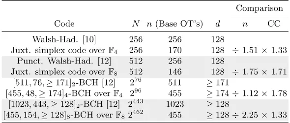
means tight in general. We now consider concrete examples of codes, that will be summarized in Table 1.
5 Shortening a code at positionsi
Comparison
Code N n(Base OT’s) d n CC
Walsh-Had. [10] 256 256 128
Juxt. simplex code overF4 256 170 128 ÷1.51×1.33
Punct. Walsh-Had. [12] 512 256 128
Juxt. simplex code overF8 512 146 128 ÷1.75×1.71 [511,76,≥171]2-BCH [12] 276 511
≥171
[455,48,≥174]4-BCH overF4 296 455 ≥174÷1.12×1.78 [1023,443,≥128]2-BCH [12] 2443 1023 ≥128
[455,154,≥128]8-BCH overF8 2462 455 ≥128÷2.25×1.33
Table 1.Comparison of using binary and q-ary codes for OT-extension. In the last two columns we consider the decrease in the number of base OT’s and increase in the dominant term of the communication complexity in the encoding phase when we consider aq-ary construction.
Remark 1. After publication, the authors have been made aware of another work [13], whose consistency check communicates fewer bits than in [12]. They achieve this by essentially having the receiver sum the columns of ˜T before sending it to
S (i.e. the receiver would send in step 3(b) of our description ˜T·1n where1n is
the all-one vector of lengthn), after which the check in step 3(c) is replaced by one in which both sides of the equation are multiplied by 1n. This can also be used in the caseq6= 2. Since our comparisons focus on the encoding phase of [12], this comparison applies to [13] as well since the encoding phases are identical.
Small values ofN
For relatively small values of N (N < 1000), [10] suggests the use of Walsh-Hadamard codes, with parameters [2k0, k0,2k0−1]
2, while [12] improves on this by using punctured Walsh-Hadamard codes instead. Punctured Walsh-Hadamard codes (also known as first order Reed-Muller codes) are [2k0−1, k0,2k0−2]
2-linear codes. These are the shortest possible binary linear codes for those values ofN
andd, as they attain the Griesmer bound. In terms ofN, the parameters can be written as [N/2,log2N, N/4]2.
The natural generalization of these codes toFq are first order q-ary Reed
Muller codes, which have parameters [qk−1, k, qk−1−qk−2]q. Moreover, there is
aq-ary generalization of Walsh-Hadamard codes, known as simplex codes, which have parameters [qqk−1−1, k, qk−1]
q.
For example forq= 4, the parameters of the simplex code can be written in terms ofN as [(N−1)/3,log4N, N/4]4, and hence, for the same values ofdand
Because of the fact thatN needs to be a power ofq, in the comparison table above it will be convenient to use the juxtaposition of two copies of the same code. This means that given an [n, k, d]qcodeC0, we can obtain a [2n, k,2d]q code
by sending each symbol in a codeword twice. With respect to the examples listed in [12], we see that by choosing an adequate finite field and using juxtapositions of simplex codes, the number of OT’s gets divided by a factor slightly over 1.5, while the communication complexity increases by a somewhat smaller factor.
Larger values of N
For larger values ofN, [12] suggests using binary BCH codes. We useq-ary BCH codes instead. It is difficult to find BCH codes that match exactly the parameters (N, d) from [12] so in our comparison we have always used larger values of bothN
andd. This is actually not too advantageous for our construction since the codes in [12] were selected so that their length is of the form 2m−1 (what is called
primitive binary BCH codes, which usually yields the constructions with best parameters) and that results in a range of parameters where it is not adequate to choose primitive q-ary BCH codes. Nevertheless, in the case where the large valueN0 = 2443 is considered in [12], we can reduce the number of base OT’s needed to less than half, while the communication complexity only increases by 4/3, and in addition to that we achieve a larger valueN = 2462. Observe that, for this value ofN, with a binary code the number of base OT’s would be restricted by the na¨ıve bound n0 ≥log2N = 462 in any case (i.e. even if d= 1), while using a code overF8 we only need to use 455.
Acknowledgements
The authors wish to thank Claudio Orlandi for providing helpful suggestions during the early stages of this work, and Peter Scholl for his valuable comments.
References
1. Beaver, D.: Correlated pseudorandomness and the complexity of private computations. In: Proceedings of the Twenty-eighth Annual ACM Sympo-sium on Theory of Computing. pp. 479–488. STOC ’96, ACM (1996). https://doi.org/10.1145/237814.237996
2. Cascudo, I., Damg˚ard, I., David, B., D¨ottling, N., Nielsen, J.B.: Rate-1, linear time and additively homomorphic uc commitments. In: Robshaw, M., Katz, J. (eds.) Advances in Cryptology – CRYPTO 2016. pp. 179–207. Springer Berlin Heidelberg, Berlin, Heidelberg (2016)
4. Frederiksen, T.K., Jakobsen, T.P., Nielsen, J.B., Trifiletti, R.: On the complex-ity of additively homomorphic uc commitments. In: Kushilevitz, E., Malkin, T. (eds.) Theory of Cryptography. pp. 542–565. Springer Berlin Heidelberg, Berlin, Heidelberg (2016)
5. Goldreich, O., Micali, S., Wigderson, A.: How to play any mental game. In: Pro-ceedings of the Nineteenth Annual ACM Symposium on Theory of Computing. pp. 218–229. STOC ’87, ACM (1987). https://doi.org/10.1145/28395.28420
6. Impagliazzo, R., Rudich, S.: Limits on the provable consequences of one-way permutations. In: Proceedings of the Twenty-first Annual ACM Sym-posium on Theory of Computing. pp. 44–61. STOC ’89, ACM (1989). https://doi.org/10.1145/73007.73012
7. Ishai, Y., Kilian, J., Nissim, K., Petrank, E.: Extending Oblivious Transfers Efficiently, pp. 145–161. Springer Berlin Heidelberg, Berlin, Heidelberg (2003). https://doi.org/10.1007/978-3-540-45146-4 9
8. Keller, M., Orsini, E., Scholl, P.: Actively secure ot extension with optimal overhead. In: Gennaro, R., Robshaw, M. (eds.) Advances in Cryptology – CRYPTO 2015. pp. 724–741. Springer Berlin Heidelberg, Berlin, Heidelberg (2015)
9. Kilian, J.: Founding crytpography on oblivious transfer. In: Proceedings of the Twentieth Annual ACM Symposium on Theory of Computing. pp. 20–31. STOC ’88, ACM (1988). https://doi.org/10.1145/62212.62215
10. Kolesnikov, V., Kumaresan, R.: Improved OT Extension for Transferring Short Secrets, pp. 54–70. Springer Berlin Heidelberg, Berlin, Heidelberg (2013). https://doi.org/10.1007/978-3-642-40084-1 4
11. MacWilliams, F., Sloane, N.: The Theory of Error-Correcting Codes. North Holland, 1 edn. (1983)
12. Orr`u, M., Orsini, E., Scholl, P.: Actively Secure 1-out-of-N OT Extension with Ap-plication to Private Set Intersection, pp. 381–396. Springer International Publishing, Cham (2017). https://doi.org/10.1007/978-3-319-52153-4 22
13. Patra, A., Sarkar, P., Suresh, A.: Fast actively secure OT extension for short secrets. In: 24th Annual Network and Distributed System Security Sym-posium, NDSS 2017, San Diego, California, USA, February 26 - March 1, 2017 (2017), https://www.ndss-symposium.org/ndss2017/ndss-2017-programme/ fast-actively-secure-ot-extension-for-short-secrets/