laser-driven wakefields:
Acceleration limits and asymmetric
plasma waves
laser-driven wakefields:
Acceleration limits and asymmetric
plasma waves
Dissertation
an derFakultat f¨ ur¨ Physik
derLudwig-Maximilians-Universitat in¨ M¨unchen
von
even when you take into account Hofstadter’s Law
beschleunigung in laser-getriebenen Plasmawellen. Hoch-intensive Laserpulse k¨onnen effizient eine Plasmawelle treiben, die elektrische Felder von 100 GV/m aufrecht er-halten kann. Da diese Felder 3-4 Gr¨oßenordnungen st¨arker sind als in Radiofrequenz-Beschleunigern, kann die ben¨otigte Beschleungiungsstrecke um den gleichen Faktor re-duziert werden, wodurch die sogenannteLaser-Wakefield Acceleration(LWFA) zu einer vielversprechenden platzsparenden, und eventuell auch billigeren, Alternative wird. Die vorliegende Arbeit soll zu einem besseren Verst¨andnis des Beschleunigungsprozesses beitragen und helfen, die Elektronenparameter zu optimieren.
Die Pulse desATLAS-Lasers (25 fs, 1.8 J) am Max-Planck-Institut f¨ur Quantenoptik wur-den in eine Gaszelle mit turbulenzfreiem, station¨arem Gasfluss fokussiert. Aufgrund der guten Repoduzierbarkeit dieses Gastargets konnten Elektronenpulse sehr stabil beschleu-nigt werden. Es war daher m¨oglich, die Empfindlichkeit der Elektronenparameter auf kleine ¨Anderungen im Aufbau mit aussagekr¨aftiger Statistik zu untersuchen. Mit opti-mierten Parametern wurden Elektronenpulse mit≈ 50 pC Ladung und einer Divergenz von≈2 mrad FWHM auf Energien von bis zu 450 MeV beschleunigt.
Da die L¨ange der Gaszelle von 2 bis 14 mm variiert werden kann, war es m¨oglich, die Energie der Elektronenpulse nach verschiedenen Beschleunigungsstrecken zu bestim-men und aus deren Evolution wichtige Parameter des Beschleunigungsprozesses zu ent-nehmen. Bei einer Elektronendichte von 6,43· 1018 cm−3 wurde ein maximales elek-trisches Feld von ≈ 160 GV/m in der Plasmawelle bestimmt. Die Strecke, nach der die Elektronen von der beschleunigenden in die bremsende Phase des elektrischen Felds wechseln, - die Dephasingl¨ange - betrug 4.9 mm. Beide Werte stimmen gut mit der The-orie ¨uberein. Zus¨atzlich wurde bestimmt, welche Faktoren, bei unseren Laserparametern, die Beschleunigungsstrecke bei verschiedenen Dichten limitieren. Bei niedriger Hinter-grunddichte,im Prinzip ideal um h¨ochste Energien zu erreichen, endet die Beschleunigung sogar noch vor dem Erreichen der Dephasingl¨ange, weil der Laserpuls defokusiert. Diese Messung ist der erste L¨angenscan, der einen großen Bereich abdeckt, sogar ¨uber die De-phasingl¨ange hinaus, was eine zuverl¨assige Bestimmung der Beschleunigungsparameter zul¨asst. Mit diesem Wissen k¨onnen Gaszellenl¨ange und Elektronendichte f¨ur gegebene Laserparameter optimiert werden.
in a laser-driven plasma wave. High-intensity lasers can efficiently drive a plasma wave that sustains electric fields on the order of 100 GV/m. Electrons that are trapped in this plasma wave can be accelerated to GeV-scale energies. As the accelerating fields in this scheme are 3−4 orders of magnitude higher than in conventional radio-frequency accel-erators, the necessary acceleration distance can be reduced by the same factor, turning laser-wakefield acceleration (LWFA) into a promising compact, and potentially cheaper, alternative. However, laser-accelerated electron bunches have not yet reached the para-meter standards of conventional accelerators. This work will help to gain better insight into the acceleration process and to optimize the electron bunch properties.
The 25 fs, 1.8 J-pulses of theATLAS laser at the Max-Planck-Institute of Quantum Op-tics were focused into a steady-state flow gas cell. This very reproducible and turbulence-free gas target allows for stable acceleration of electron bunches. Thus the sensitivity of electron parameters to subtle changes of the experimental setup could be determined with meaningful statistics. At optimized experimental parameters, electron bunches of ≈ 50 pC total charge were accelerated to energies up to 450 MeV with a divergence of ≈2 mrad FWHM.
As, in a new design of the gas cell, its length can be varied from 2 to 14 mm, the electron bunch energy could be evaluated after different acceleration distances, at two different electron densities. From this evolution important acceleration parameters could be ex-tracted. At an electron density of 6.43· 1018 cm−3 the maximum electric field strength in the plasma wave was determined to be≈ 160 GV/m. The length after which the rel-ativistic electrons outrun the accelerating phase of the electric field and are decelerated again, the so-called dephasing length, was found to be 4.9 mm. Both values are in good agreement with theory. In addition, for our laser parameters, the factors that limit the ac-celeration distance at the different densities were identified. In the desirable low-density case, where in principle the highest energies can be reached, diffraction of the driver pulse stops the acceleration even before the dephasing length is reached. While plasma-length scans have been performed by other groups, e.g. [1], this is the first comprehensive scan that covers a wide range of lengths, even beyond the dephasing length, thus allowing for a reliable determination of acceleration parameters. Only with this knowledge the gas target length and electron density can be optimized for given laser parameters.
I Introduction 3
I.1 Motivation . . . 3
I.2 Concept and State-of-the-Art . . . 4
I.3 Methods for X-ray Generation . . . 5
I.4 Structure of this work . . . 6
II High-Intensity Ultra-Short Laser Pulses 9 II.1 Mathematical Description. . . 9
II.1.1 General Characterization . . . 9
II.1.1.1 Fields . . . 9
II.1.1.2 Potentials . . . 11
II.1.2 Spectrum . . . 12
II.1.3 Gaussian Beams . . . 12
II.1.4 Spatio-Temporal Phenomena . . . 13
II.1.4.1 Spatial Chirp . . . 14
II.1.4.2 Angular Chirp and Pulse Front Tilt . . . 14
II.2 Generation. . . 17
II.2.1 General Concept of High-Intensity Short-Pulse Lasers. . . 17
II.2.1.1 Grating Compressor . . . 18
II.2.1.2 Acousto Optic Programmable Dispersive Filter . . . 19
II.2.2 The ATLASfacility . . . 20
III Laser-Matter-Interaction 21 III.1 Plane Wave and Single Electron . . . 21
III.1.1 Basic Interaction of Light Fields with Particles . . . 21
III.1.1.1 A Single Electron in a Plane Wave . . . 22
III.1.1.2 Ponderomotive Force . . . 23
III.2 Laser Pulse and Plasma . . . 24
III.2.1 Ionization . . . 24
III.2.2 Plasma Properties . . . 26
III.2.3 Plasma Waves . . . 26
III.2.4 Laser-Propagation in Plasma . . . 27
III.2.4.1 Self-Focusing . . . 28
III.2.4.3 Analytical Approaches to LWFA . . . 32
III.2.4.4 Limitations . . . 36
Electron Dephasing•Laser Energy Depletion•Laser Diffraction III.3 Electron Injection . . . 38
III.3.1 Wave Breaking and Self-Injection . . . 39
III.3.2 Ponderomotive Injection . . . 40
III.3.3 Beat Wave Injection . . . 41
III.3.4 Density Transitions . . . 41
III.4 Beamloading . . . 42
III.5 The Bubble Regime . . . 42
III.5.1 General Description . . . 42
III.5.2 Scaling Theory . . . 46
III.5.3 Beamloading . . . 49
III.5.4 Transverse focusing and Betatron Oscillations . . . 49
IV Previous Results 53 V Basic Experimental Setup 55 V.1 Overview . . . 55
V.2 Electron Spectrometer . . . 56
V.3 Charge Calibration . . . 58
V.4 Gas Target . . . 61
V.5 Beam Path Alignment . . . 64
V.6 Diagnostics for Electron Bunch Duration . . . 64
V.7 Self-Focusing of the Laser Pulse. . . 66
VI Evolution of Electron Beam Parameters 69 VI.1 Experimental Scan of the Acceleration Length . . . 70
VI.1.1 Procedure . . . 70
VI.1.2 General Electron Properties . . . 70
VI.1.2.1 Charge . . . 72
VI.1.2.2 Divergence . . . 73
VI.1.2.3 Double Peaks at 13 mm Gas Cell Length . . . 76
VI.1.2.4 Spectrum . . . 76
VI.1.3 Dephasing Length and Electric Field - 130 mbar . . . 77
VI.1.4 Dephasing Length and Electric Field - 50 mbar . . . 79
VI.1.4.1 Acceleration Limits . . . 82
Self-Guiding•Energy Depletion VI.1.5 Comparison to theory . . . 84
VI.1.5.1 Pressure Scan . . . 85
VI.1.5.2 Conclusion. . . 89
VI.2 Simulations of Near-Experimental Parameters . . . 91
VI.2.1 Self-Focusing . . . 91
VI.2.2 Evolution of the Electron Energy . . . 93
VII Wakefields from Tilted Driver Pulses 103
VII.1 Characteristics of an Angularly Chirped Laser Pulse . . . .103
VII.2 Experiment . . . .106
VII.2.1 Setup and Measurement Procedure . . . .106
VII.2.2 Measuring the Pulse Front Tilt . . . .108
VII.2.3 Measurement Results . . . .110
VII.2.3.1 General electron properties . . . .110
VII.2.3.2 Pointing Deviation . . . .110
VII.2.3.3 Betatron Motion. . . .112
VII.3 LWFA Simulations with a Tilted Driver Pulse . . . .113
VII.4 Comparison of Simulation and Experiment . . . .119
VII.5 Conclusion. . . .120
VIIIOutlook 123 Appendices 129 A Gaussian Parameters . . . .129
B Particle-in-Cell Simulations . . . .130
C Simulation Details . . . .133
D Experimental Length Scan - Low Density Spectra. . . .138
E Pulse Propagation with Kostenbauder Matrices. . . .141
Bibliography 145
Publications by the author 159
Introduction
I.1. Motivation
Since the first detection of X-rays by Wilhelm R¨ontgen in 1895 [2] this high-energy ra-diation became indispensable both in diagnostics of biological and medical samples and in material science or condensed matter physics. Nowadays, over one decade after the first cathode-ray experiments, X-ray sources are available for research applications that offer directed high-quality X-ray beams with outstanding characteristics in photon num-bers, spatial coherence and wavelength accuracy. These are synchrotron sources, where, in early days, the X-rays were only a by-product of the electron acceleration on a circular path, in later generations, however, dedicated insertion devices, such as bending magnets, wigglers or undulators are used for controlled X-ray generation. Such facilities can be found all over the world, e.g. DESY (Hamburg, Germany),BESSY (Berlin, Germany),
ESRF (Grenoble, France),LBNL (Berkeley, USA),SOLEIL (Paris, France). Their light is used to investigate the atomic structure of biomolecules, e.g. for drug development, or of promising new materials. But even the most original application of X-rays, the imaging of inner details of the human body, could still be improved by means of these brilliant X-ray sources. Instead of observing the variations in intensity of the transmit-ted X-rays, the phase of these spatially coherent beams can be evaluatransmit-ted, which contains more detailed information despite lower required dose deposition. For example, cancer patients could benefit from phase contrast imaging [3] as the high resolution might allow the discovery of tumors before they metastasize. However, especially this last application of synchrotron radiation immediately illustrates the large disadvantage of these sources. They are large-scale, cost-intensive facilities that are operated, funded and used by in-ternational collaborations. Small-scale laboratories or even hospitals cannot afford their own synchrotron sources due to both spatial and monetary restrictions. The crucial part of synchrotrons in this context is the electron accelerator. The maximum achievable ac-celerating fields in radio-frequency cavities are limited to several 10 MV/m which results in kilometers of acceleration distance in order to reach GeV-scale electron energies.
0 1 2 3 4 5 6 7 8 9
0 0.1 1 10
Electr
on Density (arb
. u.)
Laser Inten
sity (arb
. u.)
20 µm
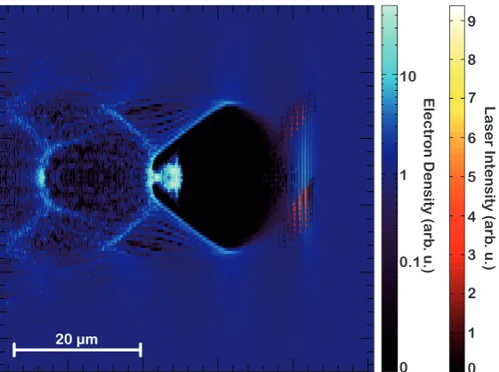
Figure I.1.:Concept of laser-wakefield acceleration in the non-linear bubble regime. In red, the intensity distribution of the laser pulse is shown, the blue color scale encodes the electron density.
100 GV/m, which allows for a reduction of acceleration length by up to four orders of magnitude. Such plasma waves can be excited by a high-intensity laser pulse and elec-trons of sufficient initial momentum may be trapped inside this wake and efficiently accel-erated to ultra-relativistic energies. Thus so-called laser-wakefield acceleration (LWFA) might become a key feature in future electron accelerators, especially if size and costs play an increasingly important role.
I.2. Concept and State-of-the-Art
The idea to accelerate electrons to relativistic energies in a laser-driven plasma wave has been first brought up by Tajima and Dawson [7] in 1979. The development of chirped-pulse-amplification [8] (also II.2) in 1985 has then lead to a leap in laser intensity that made first experimental studies possible. For the first time, laser-driven wakefield accel-eration was successfully demonstrated in 1993 by Clayton et al. [9] with an externally injected electron bunch of 1.5 MeV. In the following years several groups managed to accelerate electrons to energies above 100 MeV within only a millimeter (e.g. [10] and references therein). The acceleration regime that could be accessed with lasers of that time with picosecond pulse durations is called self-modulated laser-wakefield accelera-tion (SM-LWFA) . The advantage over earlier experiments was, that electrons from the plasma background were self-injected into the plasma wave, but only thermal broadband energy spectra could be achieved. In 2002 Pukhov and Meyer-ter-Vehn [11] predicted a highly non-linear regime, that -in simulations- lead to mono-energetic electron bunches. This so-called bubble regime may be accessed when the driving laser-pulse length is comparable to half the plasma wavelength and the a normalized vector potential of the pulse isa0 > 1. The advance in high-power ultra-short-pulse lasers allowed for the first
experimental generation of laser-driven quasi-monoenergetic electron bunches in 2004. Faure et al. [12], Geddes et al. [13] and Mangles et al. [14] independently demonstrated laser-accelerated 100 MeV-electron bunches with a relative energy spread of only a few percent and 100 pC of charge. This great breakthrough triggered a broad range of tech-nological improvements to the acceleration scheme. Among other an external guiding channel could push electron energies to 1 GeV energies [15, 16], and sophisticated injec-tion methods helped to further reduce the energy spread. For example, Rechatin et al. [17] achieved 10 pC electron bunches at 200 MeV with a 1% FWHM relative energy spread by injecting the electrons with a counter-propagating colliding pulse. Also the stability of the acceleration process and the shot-to-shot reproducibility was massively enhanced, due to advances in laser technology and improved gas targets [18], but also due to an increased awareness of the influences of the different experimental parameters on the electron beam quality. The experiments done in the frame of this thesis use a steady-state flow gas cell, that delivers extremely reproducible electron bunches, to study some of these influences. More information on the current state of experimental and theoretical research can be found in the first part of the thesis where the basics of laser-wakefield acceleration are discussed in detail.
I.3. Methods for X-ray Generation
an application of the electron bunches described in this work:
• X-ray radiation from betatron oscillations of the electrons in the focusing fields of the bubble is a by-product of the acceleration process (cf. section III.5.4). No fur-ther setup is needed. ”Bubbletron” radiation has been measured and characterized e.g. by [20].
• Alternatively, an undulator can be used for the generation of bright X-rays. An undulator consists of alternating magnets, that force the electrons on an oscillatory path. The electrons emit radiation at a wavelength that is mainly determined by the undulator period shortened by a factor of 1/γ2 (E = γmc2 is the electron energy).
First proof-of-principle experiments have been conducted with our setup [21] where soft-X-ray radiation down to 7 nm was detected from 210 MeV electron bunches. • In a next step one can think about building a table-top X-ray FEL with a laser-driven
electron source [22]. However, for this ambitious goal, the electron bunch quality still has to be drastically improved (also see chapter VIII).
• A last possibility to generate X-rays is via Thomson scattering [23, 24]. In this scheme as laser pulse is scattered from the relativistic electron bunch. Thereby the photon energy is up-shifted by a factor of γ2. The formalism describing this pro-cess is very similar to the generation of undulator radiation. However, in Thomson scattering, the basic length scale that determines the final X-ray wavelength is the laser wavelength (∼ 1µm) which is significantly smaller than the undulator period (0.5−2 cm). Thus, with moderate electron energies, extremely high-energy X-rays or even gamma-rays can be generated.
X-ray radiation from all these sources, just as from conventional synchrotrons, is ex-tremely directed (opening cone∼ 1/γ) and to a certain degree spatially coherent.
I.4. Structure of this work
The experiments described in this work help to understand some basic dynamics of laser-wakefield acceleration. This is important to be able to improve the electron bunch param-eters and their reproducibility. One presented measurement uses a variable-length gas cell to scan the evolution of the electron properties during the acceleration process. Basic pa-rameters such as the dephasing length and accelerating field strength are extracted. In the second experiment a laser pulse with tilted intensity front is used to excite the wakefield. It is demonstrated that this asymmetry leads to a deflection of the electron bunch from the original propagation axis. Furthermore, simulations show that in this case electrons are injected into the bubble at an off-axis position, probably leading to enhanced betatron oscillations.
• First the basic properties of a typical high-intensity laser pulse as it is used for LWFA are explained. A special focus lies on spatio-temporal distortions of the pulse, as those will be important for one of the experiments (section II.1).
• Subsequently, a brief overview over the practical generation of ultra-short laser pulses is given (section II.2).
• The next part discusses the theory of laser-wakefield acceleration. Starting from the very basic interaction of a single electron with a plane light wave, the pondero-motive force of a laser pulse is derived, which eventually can lead to the excitation of plasma waves. The analytical 1D wakefield theory and its consequences are de-tailed. Some limitations and scalings for the 3D non-linear regime are cited that were deduced from PIC-simulations (chapter III).
• After the theoretical discussion of the underlying physical processes, the experi-mental setup is described in detail (chapter V).
High-Intensity Ultra-Short Laser Pulses
Laser-wakefield acceleration is driven by ultra-short high-intensity laser pulses. As an example the laser facility used for the presented experiments generates ≈ 23 fs pulses with ≈ 1.7 J energy (75 TW peak power), resulting in focused peak intensities of ≈ 1· 1019 W/cm2 (for f/22 focusing optics). The electric field strength of these pulses is
on the order of 10 TV/m and electrons wiggling in these fields reach relativistic energies. In the following, the basic characteristics and generation methods of ultra-short high-intensity laser pulses will be described. The objective of the experiments in chapter VII is to analyze the influence of a driver pulse with a tilted intensity front. Therefore a special focus in the description below lies on possible spatio-temporal distortions (such as pulse-front tilt) and their occurrence during the laser pulse generation.
II.1. Mathematical Description
The concepts compiled in this chapter and additional information can be found in e.g. Jackson [25], Rulliere [26], Pretzler [27] and Wollenhaupt et al. [28].
In the following descriptions, vector quantities are indicated by bold characters.
II.1.1
General Characterization
II.1.1.1 Fields
A laser pulse can be described in the space-time domain by an electro-magnetic fieldE,B oscillating with the carrier angular frequencyω0multiplied by a spatially and temporally
confined envelopeEA,BA.
E(x,t)= EA(x,t) cos (ω0t− kx+ϕ0)
B(x,t)= BA(x,t) cos (ω0t− kx+ϕ0) (II.1)
Here,EAandBAdefine the respective polarization direction and amplitude, and the wave
40 30 20 10 0 10 20 30 40
1.5
1.0
0.5
0 0.5 1.0 1.5 2.0 2.5 3.0
1.5
1.0
0.5
0 0.5 1.0 1.5 2.0 2.5
x103
tfs
E
Field
arb
.units
Intensity
arb
.units
Intensity
EField
Envelope EField
t
Figure II.1.:Oscillating electric field and Gaussian envelopes and intensity envelope of a laser pulse with a carrier wavelength ofλ0 = 800 nm, a pulse duration of∆t =25 fsFWHM (defined by the intensity envelope) andϕ(t)=0.
ϕ0 represents an absolute phase. In vacuum, the E- and B-field oscillate in phase and
E⊥ B,E⊥ k, B⊥ kandBA = EA/c. Furthermore, the angular frequencyω0of the field
oscillation is related to its wavelengthλ0viaω0 =2πc/λ0.
The intensity I, which is defined as the modulus of the energy flux density averaged over the timeT of one oscillation period, can be measured more easily than the field itself, and is the physically important parameter in many processes.
I =0chE2iT [I]=W/m2 (II.2)
Figure II.1 shows the temporal dependence of the electric field and the intensity of a pulse with a Gaussian envelope
EA(t)= E0·e−t
2/τ2
0 (II.3)
Here τ0 represents the pulse duration given as the 1/e half-width of the Gaussian
enve-lope of the electric field. Details on the different pulse length and width definitions of a Gaussian pulse are found in appendix A. The complete 3-dimensional envelope is often assumed to be Gaussian in all dimensions:
EA(x,t)= E0·e−t
2/τ2 0 ·e−x
2/w2
x,0 ·e−y
2/w2
y,0 (II.4)
Here, x = (x,y,z) and the pulse propagates alongz = ct. wx,0 (wy,0) determines the 1/e
beam size in x (y)-direction (appendix A) andE0is the maximum field amplitude.
Maxwell equations
∇ ·E=0 ∇ ×B= 1
c2 ∂E
∂t (II.5)
∇ ×E=−∂B
∂t ∇ ·B= 0 (II.6)
and the wave equation:
∂2 ∂t2 −v
2∇2
!
Ξ(x,t)=0 (II.7)
wherevis the propagation velocity of the wave. This equation is satisfied by the E- and B-field (Ξ∈[E,B]), if
k= ω
v =
ωη
c (II.8)
whereηis the refractive index of the medium. In vacuum by definitionη= 1 andv= c. The fields of an electro-magnetic wave can also be described by associated potentials
A,Φ(see next paragraph). These must also satisfy the wave equation (Ξ∈[A,Φ]).
II.1.1.2 Potentials
A light pulse can also be described by a vector potential Aand a scalar potentialΦ that are related to the fields (II.1) by
E=−∂
∂tA− ∇Φ
B=∇ × A (II.9)
Two of the Maxwell equations (II.6) are automatically satisfied by this definition1. The
other two Maxwell equations (II.5) with the fields substituted by the potentials as in (II.9) give a new complete set of two equations that is equivalent to the four equations for the fields. For the potentials there exists a gauge freedom, i.e. different potentials connected by a scalar function f(x,t) can lead to the same fields.
If AandΦfulfill the Lorentz gauge condition, they also solve the wave equation (II.7), ∇ · A+0
∂
∂tΦ =0 (II.10)
A solution to this set of equations in the absence of charge and current is: A(x,t)=−AAsin (ω0t− kx+ϕ0)
Φ(x,t)≡0 (II.11)
where
AA =
1
ω0 EA =
c ω0
BA (II.12)
1These are the homogeneous Maxwell equations, if the general expressions with currents and charges
II.1.2
Spectrum
As the light pulse can be described as a product of a pure sinusoidal (’oscillating’) term and an envelope, the spectrum is given by the convolution of the Fourier transform of each. The oscillating term only fixes the central frequencyω0, whereas the envelope determines
the shape and the width of the spectrum. For a Gaussian envelope, the Fourier transform is again Gaussian with a spectral width∆ωthat is larger for shorter pulse durations∆t. Changing to a complex description of the light pulse facilitates the Fourier transform.
E(t)= EA(t) cos (ω0t+ϕ0)
= 1 2 h
˜
E(t)+E˜∗(t)i with E˜(t)= EA(t)ei(ω0t+ϕ0) (II.13)
The E-field can then be described as the integral over its Fourier components: ˜
E(t)= √1 2π
Z +∞ −∞
˜
E(ω)eiωt dω and E˜(ω) = √1 2π
Z +∞ −∞
˜
E(t)e−iωt dt (II.14) Still, the real physical conditions, the real temporal evolution and spectral content and shape of the pulse, are depicted by the real part of both ˜E(t) and ˜E(ω).
For the fields given above, where there are no higher order time dependencies in the oscil-lating term, the pulse is called transform-limited. In this case the time-bandwidth product is smallest: τ0 · σω = 2 (if τ0 and σω are the Gaussian widths of the envelopes of the
electric field) or∆t·∆ω= 2.77 (for FWHM quantities∆t, ∆ωof a Gaussian intensity en-velope). If there are higher order phase terms, leading to a time-dependent instantaneous frequency, the pulse is called ”chirped”. The pulse duration and thus the time-bandwidth product of a chirped pulse is larger than in the transform-limited case.
II.1.3
Gaussian Beams
Laser pulses are often approximated by a Gaussian beam profile
E(x)=E0·
exp (−ikz−ϕ(z))
w(z) exp −
x2+y2 w(z)2 −i
π λ
x2+y2 R(z)
!
(II.15)
Here, ϕ(z) denotes a phase shift (Guoy shift), R(z) is the beam radius of curvature, and
w(z) is the transverse spot size at a position z along the beam path. A Gaussian beam propagating in free space has exactly one waistw0, where the spot size is smallest and is
fully characterized byλ andw0. The distance after which the transverse beam area has
doubled in size is called the Rayleigh length and is given by
lr=
πw2 0
λ (II.16)
which determines all other parameters
w(z)= w0
s
1+ z
lr
!2
R(z)= z+ l 2
r
w0
w(z)
lR
z r
E(r)
Figure II.2.: Schematic of a Gaussian beam with Rayleigh length lR, waist w0 and divergence
angleθ
The depth of focus of the beam, also called the ”confocal parameter” is defined as twice the Rayleigh length. The Gaussian waist widthw0 and the FWHM spot size∆xare
con-nected by∆x = √2 ln (2)w0 (note that∆xis defined by the intensity envelope andw0 by
the field envelope), see also appendix A.
II.1.4
Spatio-Temporal Phenomena
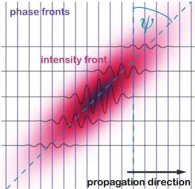
In one of the experiments presented in this work the influence of laser pulses with a tilted intensity front on the acceleration process is studied. Although the phase fronts are per-pendicular to the propagation direction, the intensity front is tilted, i.e. the peaks of every longitudinal lineout through the intensity envelope arrive at different temporal delays (see figure II.3). The ”pulse front tilt” belongs to the class of spatio-temporal pulse distortions, which therefore will be described in detail in this section. The three types, angular and spatial chirp and pulse front tilt, are closely connected.
Up to now, it was assumed that the temporal amplitude Et(t) and the spatial amplitude
Ex(x) are completely separable and functions of one variable. The same holds for the
cor-responding amplitudes in the Fourier space: the spectral amplitude
Eω(ω)=F(Et(t)) and Ekx(kx)=F(Ex(x)).
If there are spatio-temporal distortions present, the combined amplitudesE(x,t),E(kx, ω), E(x, ω) become inseparable functions of two variables, where the spatial and spectral di-mension is coupled [29]
E(x,t) =Ex(x) ·Et(t+
dt0
dx(x− x0)) Pulse front tilt (II.17a) E(kx, ω)=Ekx(kx+
dkx0
dω(ω−ω0),ky,kz)·Eω(ω) Angular chirp (II.17b)
E(x, ω) =Ex(x+
dx0
dω(ω−ω0),y,z) ·Eω(ω) Spatial chirp (II.17c)
For the sake of simplicity only one transverse spatial dimension (x) is affected and the small influences on the longitudinal dimension are neglected.
phase fronts
intensity front
propagation direction
Figure II.3.:Schematic of a tilted pulse front.
II.1.4.1 Spatial Chirp
Equation (II.17c) describes a spatial separation of the different frequencies transverse to the propagation direction. Quantitatively, the spatial chirp is characterized by either the spatial dispersionξ= dx0/dω[30] or the frequency gradientυ =dω0/dx:
If Ex(x) andEω(ω) are two Gaussian functions with a Gaussian width ofw0 andσω (cf.
appendix A), respectively, then the frequency gradient is given by [30]:
υ = ξ2+ξ (w0
σω)
2 (II.18)
It has to be noted that υ and ξ are not simply inverse functions. Whereas ξ is only de-termined by the optical system itself (gratings, imaging, see section II.2), υadditionally depends on the properties of the input pulse (w0,σω). This description is analogous in the
case of a temporal chirp where the respective relations are between time and frequency domain.
The presence of a spatial chirp in an ultra-short laser pulse causes a local reduction in bandwidth (σω → σ0ω), leading to an increased pulse duration. Also the transverse spot
size is enlarged (w0 → w00) due to the spatial separation of the different frequencies. The
new quantities are given as:
σ0 ω =
" 1 (σω)2 +
ξ2
(w0)2
#−12
(II.19)
w00=
" 1 (w0)2
+ υ2 (σω)2
#−12
(II.20)
II.1.4.2 Angular Chirp and Pulse Front Tilt
Figure II.4.:Schematic of an angular chirp. Different colors propagate under different angles.
for example if a short laser pulse hits a diffraction grating or a prism. In a chirped-pulse-amplification laser system these are essential components (see section II.2) and therefore an angular chirp can easily occur if the alignment is not perfect.
The angular chirp is usually not expressed by dkx/dωas in (II.17b) but more intuitively as
dα/dλ, whereαis the angle between the propagation direction of the whole pulse and the direction of the virtual phase front of a certain wavelength component (see e.g. [31, 32]). The angular chirp introduced by a single grating with groove spacings, diffraction angle
βand diffraction ordermis [33]:
dα dλ =
c·g λ0
withg= dkx
dω =
mλ2 0
c·scosβ (II.21)
A pulse front tilt (PFT) is a tilt of the intensity envelope relative to the optical axis as can be seen in fig. II.3. The phase front, however, remains unaltered, perpendicular to the propagation direction.
Considering expressions (II.17a) and (II.17b) representing a pulse front tilt or an angular chirp , respectively, it can easily be shown, that in most cases both descriptions are equiv-alent and only two different aspects of the same effect.
(II.17b) is the double Fourier transform of (II.17a) withω →tand kx → x. As the
distor-tion termdkx0/dωin (II.17b) includes both coordinates, it is involved in both steps of the Fourier transform. According to the shift theorem2 (e.g. [34]) the frequency-dependent
”shift” in the spatial wave vector (=angular chirp) turns into a phase in thex−ωdomain, which again - with the second Fourier transform - is converted into a time-dependent shift in space (=pulse front tilt).
Not-affected coordinates are neglected: ˆ˜
E(kx, ω)= =Eˆ˜0(kx+g(ω−ω0), ω)
˜
E(x, ω)=F−1( ˆ˜E(kx, ω)kx→x =E˜0(x, ω)e
ig(ω−ω0)x
E(x,t)=F−1( ˜E(x, ω))ω→t =E(x,t+gx) (II.22)
The simple argument as it is given above is only valid if there are no other effects present that couple the different coordinates. A spatial chirp, for example, couples x and ω as seen in (II.17c). The Fourier transform can then not be calculated in the shown way. As a consequence, an angular chirp indeed always causes a pulse front tilt, but a pulse front tilt can not only be created by an angular chirp. Also a combination of spatial and temporal chirp can have the same effect.
Another way to look at the AC-PFT equivalence is to consider the difference in spec-tral phase φ(x, λ) that an angular chirp introduces (cf. [31]). As can be deducted from figure II.4
∆φ(x, λ)≈ 2π
λ α(λ)(x−x0) (II.23)
and therefore a linear phase chirp component
dφ dλ
λ
0 = 2λπ
0 dα dλ
λ
0
(x− x0) (II.24)
depends on the spatial position x− x0. Consequently, also the group delay Dg(ω) varies
with the transverse position:
Dg(ω)=
λ0 c
dα dλ
λ
0
(x− x0) (II.25)
If the group delay of the pulse linearly increases with the transverse positions, it means that the intensity envelope is tilted relative to the propagation direction.
The PFT angle in the near field of the beamψis then given by [35]
tanψ=λ0dα/dλ (II.26)
Oscillator
CM CM
Ti:Al2O3
Stretcher
G G
EM
L
Compressor
G G
EM Ti:Al2O3
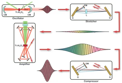
Figure II.5.:Scheme of a high-intensity CPA laser chain. CM: chirped mirror, G: diffraction grating, EM: end mirror
changed. For strong angular chirps even free space propagation can change the pulse front tilt angle [32], as the transverse separation of frequencies leads to a considerable increase of beam size and pulse duration.
More details, also about the evolution of a pulse with tilted intensity front, can be found in chapter VII and appendix E.
II.2. Generation
II.2.1
General Concept of High-Intensity Short-Pulse Lasers
(fig. II.5). The stretching/compression is done by introducing a positive/negative chirp in a controlled way (→chirped-pulse amplification), either via a pair of parallel gratings (see section II.2.1.1) or a set of prisms.
The amplification is typically achieved by pumping a Ti:Sapphire crystal with 532 nm-light (usually from a frequency doubled Nd:YAG laser) and sending the seed pulse several times through the excited crystal. For this there exist two different geometries:
regenerative amplifier: The seed pulse is coupled into a resonator by a Pockels cell,
bounces back and forth through the pumped crystal and is coupled out again after a cer-tain amount of round-trips. Advantages are the high energy boost within one amplifica-tion stage and the improvement of the transverse beam profile. Only light that matches the eigenmode of the resonator will be amplified and the cavity works as a spatial filter. The disadvantage is the high probability of amplification of spontaneous emission (ASE). This leads to a large pedestal on the timescale of the length of the pump pulse and thus bad contrast between main pulse and background.
multi-pass amplifier: The seed pulse passes through the crystal a few times in bow-tie
like geometry (see fig. II.5), no cavity is involved. Advantage: less ASE, no transmissive optics as Pockels cells or polarizers necessary, disadvantage: space consuming, geomet-rically limited number of passes.
II.2.1.1 Grating Compressor
The key parts in a CPA system are stretcher and compressor, which are based on optical setups with dispersive elements (e.g. gratings or prisms). In the complementary stretcher and compressor arrangements different spectral components of the incident pulse travel different distances leading to a positive or negative chirp of the pulse. Details on different stretcher/compressor versions can be found e.g. in Diels and Rudolph [36] or Pretzler [27]. In a grating-based system, as used in the ATLAS facility, the stretcher introduces a positive chirp, just as most transmissive optical elements in the laser chain do, and the compressor imposes a negative phase on the pulse. The compressor has to eliminate the combined spectral dispersion introduced by the strechter and the material in the amplifier chain .
G G
EM Β0 ΒΩ
Ε
d0
Figure II.6.: Grating compressor setup, G: Grating, EM: End Mirror, β0: angle of incidence,
β(ω)diffraction angle
forth, two hits on each grating) is
φ(ω)=2ω
cd0cos (β0−β(ω)) (II.27)
whered0denotes the grating separation (see fig. II.6).
A corresponding stretcher setup has to introduce a spectral phase corresponding to the compressor phase minus the phase introduced by the material dispersion, with the inverse sign. The basic geometry incorporates two exactly anti-parallel identical gratings, an imaging lens that produces a 1:1 (virtual) image of the first grating and an end mirror (cf. sketch of ”stretcher” in fig. II.5). Possible extensions of this principle include a mirror instead of the lens or a folding mirror to save one grating and reduce the size of the setup. Furthermore a roof mirror that offsets the beam horizontally or vertically can allow for more than one pass through the setup in order to introduce more dispersion.
II.2.1.2 Acousto Optic Programmable Dispersive Filter
power (TW) ∆t energy (on target)
ATLAS 25 27 37 fs 0.85 J
ATLAS 40 42 26 fs 1.1 J
ATLAS 80 74 23 fs 1.7 J
Table II.1.: Pulse parameters of the differentATLASstages. The transmission of the compres-sor plus the beamline to the target chamber was measured to be 65 %(ATLAS 40/80) or50 % (ATLAS 25), respectively.
II.2.2
The
ATLAS
facility
The presented experiments were conducted at the Advanced Titanium:SapphireLASer (ATLAS) facility. During the course of this work the parameters of ATLAS changed as two major upgrades were implemented. Table II.1 shows the pulse parameters for the dif-ferent development stages. TheATLAS facility is a Ti:Sapphire CPA system with a grat-ing stretcher/compressor+DAZZLER setup and 10 or 5 Hertz repetition rate (ATLAS 25
or ATLAS 40/80, respectively.) The ATLAS 25 setup is described and characterized in depth in [39] and [40]. Pulses (0.5 nJ) from the oscillator were pre-amplified to 1µJ and subsequently stretched to 350 ps. The 12-pass regenerative amplifier then boosted the en-ergy to 18 mJ. Two multi-pass power amplifiers then reached 0.5 J and eventually 1.7 J. After compression and propagation through the beamline a 37 fs pulse with 850 mJ total energy reached the target. The energy could be confined to the central focal spot with a Strehl ratio3 of∼ 0.7.
The front-end of ATLAS 40/70 incorporates as the new key part a MAZZLER4 within the regenerative amplifier in order to counter-act gain narrowing in the power amplifiers and therefore guarantee a larger amplified bandwidth. Thus a bandwidth 50 nmcan be sustained through the entire amplification chain. Subsequently, two (ATLAS 40) or three (ATLAS 70) bow-tie-geometry multi-pass amplifiers boost the pulse to the final maxi-mum energy of 3 J before compression (2.6 J on a daily basis). The ASE contrast5is 10−8
at 20 ps before the main pulse.
3The Strehl ratio characterizes the focusability of a laser beam. It defines the ratio of energy that is
contained in the central Airy disc of the focused beam to the energy that should be collected there if the beam profile was perfect. A Strehl ratio of 1 therefore defines a flat wavefront with a top-hat intensity distribution or if applied to characterize optical systems a completely aberration-free imaging [41].
4AMAZZLERis the same device as aDAZZLER (see section II.2.1.2) only that the transmitted beam
from the ordinary crystal axis is used. TheMAZZLER can pre-shape the spectrum of the seed pulse with a dip in spectral regions where amplification is highest. If positioned in a regenerative amplifier this leads to a uniform amplification of a broad spectral range.
Laser-Matter-Interaction
In the following sections a basic understanding of high-intensity laser-matter interactions will be established, ranging from the behavior of a single electron in an intense electro-magnetic wave to the collective dynamics a plasma wave excited by a laser pulse. Fur-thermore, the propagation of a high-intensity laser pulse in plasma is analyzed, including non-linear effects such as self-focusing. Eventually, the characteristics of laser-wakefield acceleration (LWFA) are discussed. By this mechanism electrons are efficiently accel-erated to relativistic energies in the electric field prevailing between the electron density peaks of a plasma wave.
III.1. Plane Wave and Single Electron
The basics of plasma physics and laser-matter interaction explained in the following sec-tions are composed from e.g. Goldston and Rutherford [42], Gibbon [43], Kruer [44] and Meyer-ter-Vehn and Pukhov [45].
III.1.1
Basic Interaction of Light Fields with Particles
The motion of a charged particle in an electro-magnetic field is determined by the Lorentz force:
dp
dt =q(E+ve×B) (III.1)
In the non-relativistic case v c this reduces to dp/dt = qE, as B = E/c E and thus the second term can be neglected. By integrating this equation one can obtain the maximum velocity an electron can achieve in an E-field as described in II.1: ve,quiv =
eEA/(ω0m). ve,quivis also called quiver velocity. If this velocity approachesc, neglecting
thev×B-term is not justified anymore.
In terms of the vector potential Athe equation of motion has the form:
∂p
∂t +(v· ∇)p=e ∂A
∂t −v× ∇ ×A
!
Here, the Coulomb gauge∇A=0 was used and the identityd/dt = ∂/∂t+v× ∇.
The normalized laser vector potential a0 ≡ eA/mec < 1 is considered as a rough
dis-tinction between the classical a0 < 1 and the relativistic regime a0 > 1. With a0 = 1, a
classical calculation would lead tove,quiv= c. From (II.12) it also follows
a0 = eA
mc =
λ
2π
eE mec2
(III.3)
which illustrates that the energy an electron can gain from the electric field of the laser pulse equals the rest energy of an electron fora0 =1.
III.1.1.1 A Single Electron in a Plane Wave
Although this is the most basic light-particle interaction, all other effects such as the pon-deromotive force, self-focusing or driving a plasma wave are in the end based on the behavior of each single electron in a light wave with relativistic intensities. For a com-prehensive understanding of these collective processes, the basic characteristics of this simple single-electron motion will be discussed.
According to the Noether theorem1the two symmetries of a plane wave (two-dimensional
structure and invariance under t → t− x/c) correspond to two conservation laws for the electron motion:
• The transverse momentum p⊥is always conserved.
p⊥+qA⊥=const1 for an initialp0 =0→const1= 0 (III.4)
It follows p⊥/mc=aand thus2
γ⊥=
1+a21/2 (III.5)
• For the longitudinal momentum pkit holds
E−cpk= const2 for an initialp0 =0→ const2=mc2 (III.6)
The energy of a relativistic electron in the coordinate system of the laser pulse can be written as:
E =γmc2=
q
(mc2)2+p2
kc2+ p
2
⊥c2 (III.7)
1Noether’s theorem: Every differentiable symmetry of the action of a physical system has a corresponding conservation law. The action of a physical system is the time-integral over the Lagrangian. Symmetry under a time shift gives conservation of energy, symmetry under translation in space gives conservation of momentum and rotation symmetry gives conservation of angular momentum.
2The relativisticγis defined as:
γ= p 1
1−β2 =
s
1+ p
mec !2
and β=v
and with equations (III.4) and (III.6) it follows
Ekin =mc2(γ−1)= pkc=
p2⊥ 2m =
e2A2⊥
2m (III.8)
With the definition of the normalized vector potential (III.3) and regarding the fact that a= a⊥= (ax,ay,0) it follows
γ =1+ a
2
2 (III.9)
With the aid of the derived constants of motion the integration of the equation of mo-tion (III.1) is easily done and the trajectory of a single electron in a light field (linear polarization inx-direction) is obtained as follows:
x(τ)= ca0
ω sin (ωτ) withτ= t− z(τ)
c y(τ)= 0
z(τ)= ca
2 0
4 "
τ+ 1
2ωsin (2ωτ) #
(III.10)
This trajectory consists of a drift in the light-propagation directionzdri f t(t)= a02(a20+4)−1ct
and a figure-8 motion in this drift framex=a0cω−1sin (ωτ),z−zdri f t =a0c(8ω)−1sin (2ωτ).
The electron can only gain energy from the transverse electric field. Forv≈ cthev× B -force directs this motion in the propagation direction of the laser. Still, if one imposes a symmetric temporal envelope on the electric field, the electron is at rest again after the pulse has passed. No energy is transferred. However, if this assumption of spatially uni-form light fields with a slowly varying temporal envelope is violated, the electron can indeed gain energy. For example tightly focused laser beams with strong intensity gra-dients can ”repel” electrons from the high-intensity regions. The corresponding force is described in detail in the next section. It could be experimentally verified [46] that the angleθunder which electrons are scattered out of an intense laser focus is the same angle under which an electron moves in a plane wave (with (III.8)):
tanθ= p⊥
pk =
s 2
γ−1 (III.11)
III.1.1.2 Ponderomotive Force
The interaction of a single electron with an electro-magnetic wave becomes more inter-esting, if, instead of a plane wave, one considers a spatially and temporally limited pulse e.g. with a Gaussian envelope as (II.4). As will be seen, although in principle following the electric field (quiver motion), electrons drift away from regions of higher intensity. In the limitv cthe equation of motion (III.1) for an electron in a light wave polarized along thex-direction and propagation alongzreduces to
∂vx
∂t =− e
The Taylor expansion of an electric field as in (II.1) gives
Ex(x,t)= Ex,A(x,t) cos (ϕ)+x
∂Ex,A(x,t)
∂x cos (ϕ)+. . . (III.13)
withϕ = ω0t−kzz. To the lowest order the electron directly follows the field and moves
with the quiver velocityve,quivas defined before. However, from the cycle-averaged
equa-tion of moequa-tion for the second order field *∂v(2)
x
∂t
+
T
= *
e2 m2ω2c2Ex,A
∂Ex,A(x,t)
∂x cos (ϕ)2
+
T
= e2 4m2ω2
∂E2
x,A
∂x (III.14)
the non-relativistic ponderomotive forceFp =mh∂vx/∂tican be determined (here already
for the general 3D case):
Fp =−
e2
4mω2 0
∇E2A (III.15)
It is obvious that the ponderomotive force is proportional to the gradient of the intensity
I ∝ E2A. Furthermore the ponderomotive force is a conservative force that can be derived from a potentialUpviaFp =−∇Upwith
Up =
e2
4mω2 0
E2A (III.16)
It should be noticed that the ponderomotive potential is not only proportional to the inten-sity but to Iλ20.
In the relativistic case v ≈ cthe equation of motion is best used in the form of (III.2). Assuming that again the motion can be separated into a fast oscillating part, that directly follows the vector potential p = eA (III.4) and a slow component, the relativistic pon-deromotive force can be determined (withγ =(1+(p/mc)2)1/2(III.5)):
Fp,rel =−
e2m
2γ ∇A
2 =−
mc2∇γ (III.17)
For a detailed derivation of the relativistic ponderomotive force see e.g. [47].
III.2. Laser Pulse and Plasma
III.2.1
Ionization
In the case of high-intensity laser pulses it is valid to reduce the description of laser-matter
interaction laser-plasmainteraction. By the mechanisms explained in the following sec-tion, matter is at least partially ionized already by the pre-pulses or the rising edge of the main pulse.
instantaneous laser potential
VL= -e|E|r
undisturbed binding potential
combined potential
allowed electron states
r
d
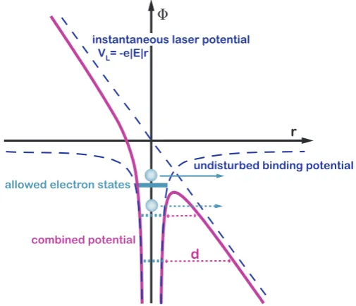
Figure III.1.:Scheme of barrier suppression ionization (highest electron state, continuous line) and tunnel ionization (lower two states, dashed lines). The instantaneous laser potential on the time-scale of ionization can be approximated to be linear in space.
a laser pulse intensity of 1.4·1014 Wcm−2, corresponding to an electric field strength of 2.4·109Vm−1, deforms the potential well that binds the electron to the proton so heavily
that the electron is immediately set free (see fig. III.1, highest electron state, continuous line). This effect is called barrier suppression ionization. If the light field is not strong enough to suppress the binding field completely below the respective occupied state still tunnel ionization can occur. The electrons can tunnel through the finite barrier with a probability that is inversely proportional to the barrier widthd (see fig. III.1, lower two electron states, dashed line). Both regimes are quantitatively characterized by the ADK-model described in Ammosov et al. [48] and Delone and Krainov [49].
For even lower light intensities this semi-classical picture is not valid anymore and the ionization mechanism changes to multi-photon ionization [50]. If the energy of one pho-ton (Ti:Sapph laser withλL = 800 nm → EL = ~ω = 1.5 eV) is not enough for direct
photo-ionization (ionization energy for hydrogenEi = 13.6 eV) the summed up energy
ofn= bEi/ELcsimultaneously incident photons can cause multi-photon ionization of the
atom. ”Simultaneously” in this case means that then+1stphoton has to arrive within the
lifetime of thenth virtual excited state, which usually is on the order of 10−14 s [51] and easily fulfilled with a finite probability for high-intensity laser pulses that deliver Joules of energy within several ten femtoseconds (1 J = 6.2· 1018 eV ≈ 4· 1018 photons at λL=800 nm).
In conclusion, it becomes clear that for focused laser intensities of > 1018 Wcm−2
III.2.2
Plasma Properties
A plasma is a mixture of neutral and charged particles or, in the case of a fully ionized plasma, only of positively and negatively charged particles. The formal definition of a plasma requests two characteristics to be fulfilled:
1. The distance over which the charge of a test particle that is inserted into the plasma is shielded out must be much smaller than the plasma size. This distance, called Debye length, is:
λD ≡
s
0kBTe
nee2(1+ZTe/Ti)
(III.18)
wherekB is the Boltzmann-factor,Te the electron temperature,Ti the ion
tempera-ture andne the electron density. This expression is only valid, if electrons and ions
each are in a thermal equilibrium among themselves. However, electrons and ions do not necessarily have to be in a thermal equilibrium with each other.
This condition can also be regarded as quasi-neutrality, i.e. on a length scale> λD
the plasma appears to be electrically neutral.
2. There must be 1 particles within a Debye sphere of radiusλD:
ne·
4 3πλ
3
D 1 (III.19)
If the Debye sphere is densely populated, the plasma is called weakly coupled; the plasma then is hot and diffuse and collective effects can occur as Coulomb scattering between particles is rare. For strongly coupled plasmas a different formalism has to be applied.
In laser-wakefield acceleration of electrons the plasma before the laser arrival is as-sumed to be weakly-coupled and quasi-neutral. During the interaction of the laser with the plasma only electrons are affected. The heavier protons and ions form an immobile background, as the normalized vector potential for protons isa0,p =eA(mpc)−1 1
It has to be noted that the interaction with a femtosecond laser pulse happens on a time scale τint that is much smaller than the mean free time between collisions τc in such a
plasma. Even for solid state plasma densitiesτc/τint ≈ 40 [52]. Consequently, collisions
can be neglected when treating relativistic interactions between ultra-short laser pulses and plasma. On the other hand the electron population cannot be in a thermal equilib-rium during the interaction. Applicable simulation codes account for both conditions (see appendix B).
III.2.3
Plasma Waves
other side. On the time scale of this oscillation the ion background does not respond to the generated electric fields as its inertia is too high. The oscillation frequencyωp of a
cold plasma is governed by the restoring force and thus dependent on the electron density:
ωp =
s
nee2
0m
(III.20)
and the plasma wavelength isλp =2πc/ωp. mis the electron mass.
For general Langmuir waves in a warm plasma the ”Bohm-Gross dispersion relation” is valid:
ω2
L =ω
2
p+3
kBTe
m k
2
L (III.21)
whereT is the plasma temperature andkL =c/ωLthe wave vector of the Langmuir wave.
At low temperature or long wavelength (lowk) the phase velocityωL/kL can grow
arbi-trarily large, but the group velocity∂ω/∂k approaches zero, so no energy or information can propagate. At short wavelengths (largek) or high temperatures, however, group and phase velocity both converge to √3kBT/mand the wave propagates forward. This is very
important for the subject of laser-wakefield acceleration as energy transfer is possible be-tween propagating plasma waves and charged particles that move at velocities close to the wave phase velocity (Landau damping). If the plasma wave is driven by a laser pulse, the phase velocity of the plasma wave corresponds to the group velocity of the laser pulse (see section III.2.4)
Langmuir waves are purely longitudinal, electrostatic waves. Only if the wave has trans-verse components also magnetic fields can oscillate. If the wave is excited by a high-intensity few-cycle laser pulse, electrons are displaced both longitudinally and trans-versely relative to the laser propagation axis and the resulting electromagnetic oscillation incorporates a complex three-dimensional structure (see section III.5).
III.2.4
Laser-Propagation in Plasma
The characteristics of plasma-light interactions differ depending on the ratio of ωp/ωl
(where ωl is the frequency of the incident light). If ωp < ωl the light can propagate
through the plasma. Then the plasma is called undercritical or underdense (asωp ∝
√
ne).
Ifωp > ωlthe light is reflected and enters the plasma only to the skin depth on the order
ofc/ωp. In the overcritical case the resonance frequency of the plasma electrons is higher
than the frequency of the driving electric field of the laser and they can easily follow the oscillation. The driving laser field is damped and the secondary dipole emission of the oscillating electrons is reflected back.
For a Ti:Sapphire laser with λ0 = 800 nm the critical density nc at which ωp = ω0 is
1.74·1021cm−3
The dispersion relation for the propagation of light in plasma is:
ω2
l =ω
2
p+c
2
which determines the refractive index of plasma for laser frequencyωl
η= s
1− ωp
ωl
!2 =
r 1− ne
nc
< 1 (III.23)
In the case of high laser intensities a0 ≥ 1 the plasma electrons gain significant energy
during the interaction with the laser. As the dispersion relation for the laser propagation in plasma is mainly determined by the electron response, this energy change must be considered. According to [53] this can be accounted for by substitutingω2
pby ˆω2p =ω2p/γ.
Due to the reduced effective plasma frequency laser pulses can then even propagate in moderately overdense plasmas. The effect is called self-induced relativistic transparency. The phase velocity of a laser pulse traveling in plasma isvl,ph =c/ηand the group velocity
is vl,gr = ηc. With (III.22) this gives a relativistic laser group velocity of vl,gr = c(1−
ω2
p/(γ2ω20))
1/2. The phase velocity of a plasma wave excited by a laser pulse is equal to
the group velocity of the laser. Hence, theγp,phof the plasma electrons can be determined
to
γp,ph=
1 q
1− vl,gr
c
= ω0 ωp
γ (III.24)
III.2.4.1 Self-Focusing
As a laser pulse witha0 ≥1 propagates through an underdense plasma background,
elec-trons quiver with relativistic relativistic and the instantaneous energyE = γmc2depends on the laser intensity. Asγdirectly enters into the refractive index (III.23), this leads to a reduced phase velocity in regions of high laser intensities. In addition, the ponderomotive force (III.17) of the laser pulse is directed along the intensity gradient and thus expels electrons from the central high intensity zone. This generates a density gradient, with lower densities, meaning higher refractive index, in regions of higher laser intensity. Both effects lead to a transverse plasma profile with high refractive index on the optical axis and lowerηoff-axis that is generated by the very front part of the laser pulse and acts as a lens for the main part. The effect is even enhanced during propagation as focusing of the pulse increases the focal power of the ”lens”. This so-called self-focusing counteracts the beam diffraction and can lead to self-guiding of the laser pulse over several Rayleigh lengths. Of course, also external guiding channels can be formed by e.g. additional laser pulses or an electric discharge.
If no external guiding channel is used, self-guiding is desirable as the interaction length with high laser intensities, that are only available in the focal spot, can be extended be-yond the Rayleigh length.
Longitudinal/temporal self-modifications due to intensity-dependent changes in the index of refraction will be discussed in the next section. In order to achieve proper guiding of a Gaussian beam with waist w0, the plasma channel must exhibit a parabolic transverse
profile of depthδnch =(πrew20)−1(e.g. [54]) or normalized to the initial plasma density
re =1/(4π0)e2/(mc2) is the classical radius of an electron. In general the index of
refrac-tion in a plasma with a spatially slightly varying density ˜neis given by
η(r,z)= s
1− ω
2
p
ω2 0
˜
ne(r,z)
neγ(r,z)
(III.26)
If ˜ne is small, thenηcan be expanded aroundδne =n˜e−ne([55, 56, 57, 58])3:
η(r,z)=1− 1 2
ωp
ω0
!2 1− a
2 0
8 +
δne
ne
+ ∆next
ne
!
(III.27)
Here, the terma0/8 causes the change ofγof the background electrons (relativistic
self-focusing), δne is the density depletion due to the transverse ponderomotive force
(pon-deromotive self-focusing), and∆nextis a possibly preformed external plasma channel.
If there is no external guiding channel (∆next = 0), the dominant effect is the
relativis-tic mass correction. Therefore, commonly a crirelativis-tical laser power Pc for self-focusing is
deduced only from this term. Ponderomotive effects (see below) and external channels reducePc [59].
A guiding profile (III.25) is generated by the relativistic mass correction term if
a2 0
8 ≥ 4 (kpw0)2
(III.28)
Condition (III.28) for relativistic self-focusing can also be expressed in terms of laser power. In order to achieve self-guiding the power Pmust be larger than a critical power
Pc (for linear polarization):
P Pc ≥ a 2 0k 2
pw20
32 (III.29)
with
Pc = 2c
e2 r2
e
!2 ω
0 ω2
p
!2
= 17.4ω
2 0 ω2
p
[GW] (III.30)
ForP< Pcdiffraction dominates, forP>Pc the pulse is focused down until higher-order
non-linearities that are not included in this simple derivation will balance the focusing force. IfP=Pc the pulse is guided with the original spot size.
[60] gives an expression for the evolution of the focal spotw(z) size during self-focussing (withdw/dz =0 atz=0):
w(z)
w0
= 1+ 1− P
Pc ! z2 l2 r (III.31)
3The formality to handle a paraxial wave propagating in a such a refractive index distribution is similar
to non-linear optics, where the Schr¨odinger equation is solved with a third-order non-linearity. The index of refractionnof a material has a weak dependence on the intensityIof the propagating light:
n=n0+∆n(I)=n0+12n2I+. . .Asn2is on the order of 10−20m2/W, it only plays a role for high-intensity
The density variationδnedue to the ponderomotive force can be estimated from the fact
that the ponderomotive force must be balanced by the space charge force as the resulting force should be a steady-state radial force. This means that (with (III.17))∇⊥γ⊥ = ∇⊥Φ, whereγ⊥=(1+a2)1/2((III.5)), and with the Poisson equation (∇2⊥Φ = k2pδne/ne) follows:
δne
ne
= ∇2⊥(1+a2)1/2
k2
p
(III.32)
assuming that δne/ne ≤ 1. For a Gaussian laser pulse a2 = a02exp (−2r2/w20) and a < 1
this yields a density variation
δne =−δne(0) 1−2
r2 w2 0
!
exp (−2r2/w20) (III.33)
where the on-axis channel depth is
δne(0)= a20
1
πrew20
=a20δnch (III.34)
This shows already that for a0 < 1 self-guiding can not be established merely due to
density variations caused by the ponderomotive force. For laser powers that approach the critical power Pc relativistic self-focusing will dominate. Sun et al. [61] and Hafizi et al.
[62] show that the ponderomotive force can enhance the effect by slightly decreasing the threshold power for self-focusing to
Pc,r+p= 16.2
ω2 0 ω2
p
[GW] (III.35)
However, the density response termδnein the refractive index (III.27) becomes
impor-tant to the effectiveness of self-guiding for ultra-short pulses withL = c∆t < λp. Due to
the temporal/longitudinal intensity gradient of the laser pulse, the ponderomotive force at the front of the pulse also accelerates electrons in longitudinal direction, ”pushes them for-ward”. This leads to a density bump in the front region of the pulse (see also fig.III.2(b)), and thus a decrease in refractive index which almost entirely cancels the increase due to relativistic mass effects. Hence, the leading edge of a pulse always diffracts. As the time scale for the channel formation is determined by the time scale∼ω−p1on which collective plasma dynamics take place, laser pulses that are shorter than a plasma wavelengthL< λp
can not be guided efficiently, even ifP/Pc >1. However, a degree of self-guiding also for
ultra-short pulses has been observed under certain circumstances.
Decker et al. [63] showed that self-guiding of short pulses is possible for P/Pc 1.
Electrons in the leading edge of the pulse are accelerated forward with a momentum
pk = mca20/2. Ifa20 1 the electrons keep up with the leading edge of the laser pulse and constantly extract energy. This leads to 100% local energy depletion of the front part before it can diffract and to an electron-free ion channel right behind which can guide the back of the pulse (also see section III.5).
still self-guided, as long as their transverse focal spot sizew0 ≥λp. If the so-called
blow-out radius, the transverse size of the wakefield structure determined by the laser focal spot size, is too small, then the expelled electrons turn back to the laser axis within the length of the laser pulse. The resulting density variations along the laser pulse again cause mod-ulations in the pulse which can lead to instabilities or even cause the pulse to break up into several filaments.
For a0 ≥ 1 another aspect has to be considered: The laser will drive a (non-linear)
plasma wave and lose energy to the plasma (pump depletion). Therefore the guiding con-ditionP= Pcrcan only be fulfilled for a limited distance (see depletion length, paragraph
III.2.4.4), as with the pump depletion the available power decreases and for P < Pcr
diffraction dominates. If one starts withP > Pcr to obviate the energy/power loss or
be-cause it is necessary for the desired interaction, self-focussing will set in and the beam diameter will decrease indefinitely (in first order theory). One possibility to achieve stable self-guiding in the case of strong plasma wave excitation is to go to configurations where the on-axis density becomes zero due to ponderomotive expulsion of electrons from re-gions of high laser intensity. This means that the on-axis density deviation (III.34) should correspond to the initial density δne(0) = ne. With k2p = nee2/(mc20) this conditions
shortens to w0kp = 2a0, which is valid for a0 < 1. In the non-lineara0 > 1 case the
cavitation condition reads (e.g. [60]):
w0kp =2
√
a0 (III.36)
With such a combination of laser pulse and plasma parameters a stable guiding channel is formed, where relativistic self-focussing is suppressed even ifP> Pcr, merely due to the
lack of electrons in the center [65], [66]. Since further focusing cannot occur, stable guid-ing can take place inside the resultant cavitated channel. This regime also corresponds to the bubble or blowout regime of laser-wakefield-acceleration (section III.5). Additional automatic self-channeling of the laser is a welcome side-effect of the bubble regime as the electron acceleration length is not limited by diffraction.
For electron acceleration the important length is the dephasing lengthLdeph(see details in
section III.2.4.4). It has been shown in simulation [58] (also section III.5.2) and experi-ment [67] that the initial power that is necessary to self-guide a laser pulse that is driving a plasma wave (and thus continuously losing energy) overLdeph is
P0 ≥
1 8
ω0 ωP
6/5
Pc (III.37)
III.2.4.2 Temporal pulse modifications due to collective plasma dynamics
The same modulations in the refractive index responsible for self-focusing also occur lon-gitudinally along the laser pulse. The locally varying group velocity vl,gr = ηccan cause
a compression of the pulse accompanied by the generation of new frequencies in the laser spectrum (self-phase modulation). For details see e.g. [70]. This pulse shortening effect can be especially useful if the initial laser pulse is too long to resonantly drive a wakefield [71]. Faure et al. [72] measured a pulse compression from 38 fs to 10−14 fs. Schreiber et al. [73] characterized the complete temporal pulse shape including pulse steepening at the front or rear side, respectively, depending on the position in the plasma wave.
III.2.4.3 Analytical Approaches to LWFA
In the wake of the invention of high-power short-pulse lasers an analytical description of laser-driven highly non-linear plasma waves was developed. A comprehensive derivation can be found in e.g. [39]. It concludes work done by Tsytovich et al. [74], Berezhiani and Murusidze [75], Bulanov et al. [76] and Sprangle et al. [77], who managed to formulate a theory with the assumption that the group velocity of the laser equals the speed of light in vacuum (vl,gr = c). This restriction could be released later on as can be seen in the
extended work of Dalla and Lontano [78], Esarey et al. [79], Kingham and Bell [80] and Mori [56].
This fully relativistic one-dimensional plasma wakefield theory outlined below is based on the following assumptions:
• Collisions can be neglected.
• Ionization and recombination do not a play a role. • Thermal plasma effects can be ignored.
• Arbitrary laser amplitudesa0are allowed.
• Arbitrary group velocities of the laser pulseβl,gr= vl,grc−1are supported.
• The driver pulse is linearly polarized (and travels along thez-direction).
As seen before, collisions take place on a much longer time scale than the laser-particle interaction. Consequently, also recombination can be neglected. Due to the high field strength total ionization of the relevant plasma volume occurs in reality already with pre-pulses or the raising edge of the main pulse (see section III.2.1). Furthermore the quiver energy that the electrons gain from the laser field is much larger than their thermal energy.
Basically, a closed set of differential equations to gain expressions for the different plasma wave properties is derived as follows:
In the following normalized quantities are used: normalized vector potential a0 = eA(mc)−1 of the laser pulse, normalized scalar potential Φ