Finite Element Modeling of Light Frame Wood Structures An Integrated Approach

(1)

COLLINS, MICHAEL SCOTT . Finite Element Modeling of Light Frame Wood Structures An Integrated Approach. (Under the direction of Professor Bohumil Kasal).

This research aims to improve the framework and practicality for the analysis and design of light frame wood structures. The light frame wood structure is broken down into its

constituent components for modeling: connections, shearwalls and diaphragms, then the assembled structure. This work relies extensively on available finite element technologies to identify key components and modeling methods of those key components. Finite element modeling strategies were developed to investigate the response of light framed wood

(2)

by

Michael Scott Collins

A dissertation submitted to the Graduate Faculty of North Carolina State University

in partial fulfillment of the requirements for the degree of

Doctor of Philosophy

Civil Engineering

Raleigh, North Carolina 2009

APPROVED BY:

_______________________________ ______________________________

Dr. Bo Kasal Dr. Mervyn Kowalsky

(3)

DEDICATION

(4)

BIOGRAPHY

(5)

ACKNOWLEDGMENTS

(6)

LIST OF TABLES

DYNAMICALLY LOADED LIGHT-FRAME WOOD STUD WALLS EXPERIMENTAL VERIFICATION OF THE ANALYTICAL MODEL

Table 1Green Wave Parameters for Wave Channel Tests on Breakaway Walls ...41 Table 2 Moduli of Elasticity for studs in Breakaway Wall ...42 Table 3 T-beam model parameters ...44

DESIGN MODELS OF LIGHT FRAME WOOD BUILDINGS UNDER LATERAL LOADS

Table 1 Comparison of Calculated Lateral Load Distributions under Design Wind Load of 30 kN...67 Table 2 Summary of Calculated Stiffness and Measured Capacity of Test House Walls...68 Table 3 “Error” for Different Lateral Load Distribution Methods Compared to Finite

Element Model Calculation ...68 Table 4 Experimentally Applied Displacements and Measured Load Distribution in Test House ...69 Table 5 Comparison between Measured and Calculated Load Distribution under Four

Different Applied Displacement Cases (1 kN = 0.225 kips, na = not applicable) ...70

THREE-DIMENSIONAL MODEL OF LIGHT FRAME WOOD BUILDINGS. II: EXPERIMENTAL INVESTIGATION AND VALIDATION OF THE ANALYTICAL MODEL

Table 1 Parameters for Walls W1, W2, W3, and W4...83

DYNAMIC ANALYSIS OF DENSIFIED LAMINATED TIMBER FRAME

(9)

APPENDIX A

Table 1 Connection Parameters for Type III unreinforced connection ...115

APPENDIX B

MODELING OF NONLINEAR HYSTERETIC CONNECTIONS

(10)

LIST OF FIGURES

NONLINEAR HYSTERETIC CONNECTIONS

Fig. 1 Asymmetric behavior- Curve locations defined...8

Fig. 2 Variation in monotonic tests of nailed connections (Yeh et al. 1999) ...9

Fig. 3 Tests required for automated system identification (a) monotonic, (b) zero mean cyclic, (c) non-zero mean cyclic...9

Fig. 4 Comparison of monotonic and cyclic tests ...10

Fig. 5 Example of Nonlinear least squares fit vs Trial and error...12

Fig. 6 Backbone curve, yield point, and breakpoint in positive quadrant ...13

Fig. 7 Curve 2 and boundary ...14

Fig. 8 Influence of the number of cycles on force intercept...15

Fig. 9 Curve 3 boundary conditions ...16

Fig. 10 Five non-zero mean cyclic tests of reduced scale specimens...18

Fig. 11 Connection test...19

Fig. 12 Intersection of segment 5 and segment 7 ...20

Fig. 13 Comparison of model response to experiment...21

Fig. 14 Analytical Fit and Predicted Response to Arbitrary Loading (Force=kN,Displacement= cm) ...22

Fig. 15 Analytical fit for model of moment resisting joint under QSCT loading for Type III reinforced connection ...23

Fig. 16 Comparison of Analytical model of versus Experimental under Arbitrary loading for Type III glass fiber reinforced connection...24

Fig. 17 Analytical fit of model of moment resisting joint under QSCT loading for Type III unreinforced connection ...25

Fig. 18 Analytical fit of model of moment resisting joint under arbitrary loading for Type III unreinforced connection ...25

(11)

DYNAMICALLY LOADED LIGHT-FRAME WOOD STUD WALLS-EXPERIMENTAL VERIFICATION OF AN ANALYTICAL MODEL

Fig. 1 Unbroken Wave Pressure on Wall (wd=hydrostatic pressure, P1 =Pressure from

Standing Wave, SWL= Still Water Level) ...36

Fig. 2 Time Sample of Experimental and Analytical Reactions of Top and Bottom Plate for Static Loading ...37

Fig. 3 Wave Channel Setup (Yeh 1997) ...38

Fig. 4 Schematic of Strain Gauge Locations (Back View)...39

Fig. 5 Wall Configuration-Wall Profile...41

Fig. 6 T-beam schematic...44

Fig. 7 Finite Element Schematic of Breakaway Wall...46

Fig. 8 Customized Model Hysteretic Behavior and Identifying Curve Numbers ...47

Fig. 9 Failure Loading Strain and Displacement Response for T-beam vs Experiment ...50

Fig. 10 Individual Nail Response of the Sole Plate Connection for T-beam ...51

Fig. 11 Top Plate and Sole Plate reactions ...53

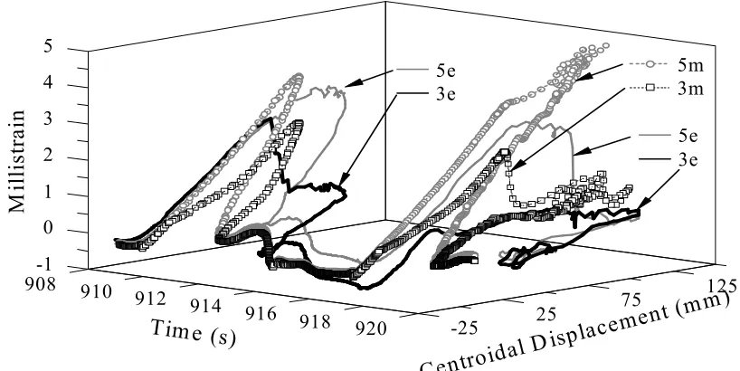
Fig. 12 Stud Millistrain vs Time (Stud s16 and S9 location shown in Fig. 4 , m=model, e=experiment)...54

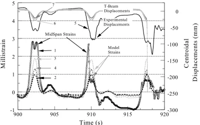
Fig. 13 Midspan Strains and Displacements vs Time ...55

Fig. 14 Nail Hysteresis for the Time period 360 to 870 seconds ...56 1 = Strain Gauge 3 (see Figure 4)

2=Midspan Strain of T-beam,

3= Midspan Strain of T-beam E=10000MPa, 4= Midspan Strain of T-beam stud E=17462MPa, 5=Displacement Transducer (see Figure 4),

(12)

Fig. 15 Nail Hysteresis for the Time Period 360 to 930 seconds ...57

Fig. 16 Stud to Sole Plate separation...58

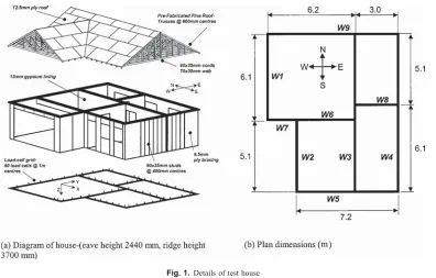
DESIGN MODELS OF LIGHT FRAME WOOD BUILDINGS UNDER LATERAL LOADS Fig. 1. Details of test house ...65

Fig. 2. Description of different load distribution methods [(a) to (h) in plan view]...66

Fig. 3. Load-displacement relationships for individual walls in test house...69

Fig. 4. Applied displacement cases used in experiments...70

THREE-DIMENSIONAL MODEL OF LIGHT FRAME WOOD BUILDINGS. I: MODEL DESCRIPTION Fig. 1. Hysteresis model with identifying curve numbers...76

Fig. 2. Finite element model of the experimental house (note: walls consist of beam, shell, and diagonal spring elements)...77

Fig. 3. Composition of finite element wall model (a) Beam Elements, (b) shell Elements (plate stiffness only), (c) hysteretic Springs, and (d) assembled wall ...78

Fig. 4. Plan view of test house with loading point locations for destructive Test (lengths in meters) ...78

Fig. 5. Three-dimensional schematic of test house with load cell grid ...78

Fig. 6. Endwall connection detail ...79

THREE-DIMENSIONAL MODEL OF LIGHT FRAME WOOD BUILDINGS. II: EXPERIMENTAL INVESTIGATION AND VALIDATION OF THE ANALYTICAL MODEL Fig. 1. Plan view of test house with loading point locations for destructive test (lengths in meters) ... 84

Fig. 2. Loading protocol used in pseudostatic destructive phase of full-scale house test (1)

(13)

Fig. 3. Comparisons of force displacement curves for (a) Wall W3 and (b) W4 – isolated test versus house results... 84 Fig. 4. Experimental versus analytical results of the force-displacement curves (north-

south direction) for (a) Wall W1 , (b) Wall W2, (c) Wall W3, (d) Wall W4 ...85 Fig. 5. Experimental versus analytical results of the force-displacement curves

(east-west direction) for (a) Wall W5 and (b) Wall W9 ...86 Fig. 6. Experimental versus analytical results for the north-south and east-west direction:

(a) Total energy dissipated versus half-cycle number; (b) cumulative energy dissipated versus half-cycle number; (c) error in prediction of energy dissipated for the north-south direction per half-cycle number; and (d) error in cumulative energy dissipated for the north-south direction per half-cycle number

(Note: energy dissipated in the north-south direction is the summation of the component of energy dissipated in the north-south direction for all the walls. Energy dissipated in the east-west direction is the summation of the component in the east-west direction for walls W5 and W9)...87 Fig. 7. Experimental versus analytical results for (a) Energy dissipated per cycle versus

half-cycle number – summation of energy dissipated for Walls W5 and W9, (b) cumulative energy dissipated versus half-cycle number – summation of energy

dissipated for Walls W5 and W9 ...88 Fig. 8. Experimental versus analytical results for the north-south walls: (a) Comparisons

of cumulative energy dissipated versus half-cycle number and (b) error in prediction of cumulative energy dissipated per half-cycle number.(Note: energy dissipated as shown is the component of dissipated energy in the north-south direction for the

respective walls) ...88 Fig. 9. Experimental versus analytical results of the undisplaced and displaced structure

at an imposed displacement of 76 mm. (displacements scaled by 25x relative to

(14)

Fig. 10. Envelope curves for Walls W1- W4 – (a) Primary Cycle, (b) secondary cycle, (c) tertiary cycle - (X-axis -- average displacement of W3 and W4, Y – axis—force in respective wall)...89 Fig. 11. Envelope curves for Walls W1-W4 as a percentage of total load – (a) Primary

cycle, (b) secondary cycle, (c) tertiary cycle - (X-axis -- average displacement of W3 and W4, Y – axis-- force in respective wall) ...89 Fig. 12. Reactions for individual load cells on Wall W2. (Wall location shown in Fig. 1.

Model results are for monotonic test with a 78 mm displacement. Dotted lines

indicate door and window openings.)...90

DYNAMIC ANALYSIS OF DENSIFIED LAMINATED TIMBER FRAME

Fig. 1 Two story laminated timber frame –experimental setup and schematics (Heiduschke 2006 and Kasal 2004) (note: h1=2600mm, h2=2400mm. Joint

dimensions are in millimeters and d= dowel)... 92 Fig. 2 Comparison of Analytical Model of Beam to Column (BC) connection...93 Fig. 3 Comparison of Analytical Model of Column to Foundation (CF) connection ...94 Fig. 4 Story accelerations of Densified Laminated Frame under seismic test for time

period of 0s to 30s...96 Fig. 5 Story Drift of Densified Laminated Frame under siesmic test for

time period of 0s to 30s ...97 Fig. 6 Comparison of experimental and analytical joint rotations...98 Fig. 7 Extent of joint rotations compared to testing protocol used for parameter

identification...99 Fig. 8 Consortium of Universities for Research in Earthquake Engineering (CUREE)

(15)

Introduction

BACKGROUND

The large majority of residential structures in the US are the light frame wood type. This type of construction is characterized by the assemblage of the substructure and the intercomponent connections between them. The substructure assemblages such as shear walls, floor and ceiling diaphragms are generally made up of dimension lumber of varying dimension constructed into simple frames and sheathed or braced to prevent racking and contribute lateral resistance for the whole structure.

Vertical loads such as snow loads are carried to the walls by the roofs and floors through out of plane bending. The walls then transfer the vertical loads to the foundation. Lateral loads such as wind loads or seismic loads are transferred through in-plane bending of the floor and ceiling diaphragms and out-of plane bending of the walls to walls inline with the applied loads. The shear loads are transferred to the foundations primarily through in-plane shear.

The connections between the parts of the substructure are typically of the dowel bearing type. This type of connection is characterized by a dowel being embedded or

withdrawn into the surrounding medium through the transfer of lateral and axial loads. This type of connection when loaded in shear is highly nonlinear under cyclic and montonic loading. Under dowel bearing the surrounding medium displays a nonlinear force deformation response. The amount of nonlinearity present in the particular substructure depends on the load orientation relative to the substructure and the substructure placement and method of attachment to the surrounding structure.

(16)

demanding if all the physical phenomena such as friction, gaps and contact forces, material aniosotropy are accounted for in the formulation. The number of nonlinear dowel

connections such as nails and bolts in light frame construction typically results in a nonlinear response of the subsystem or component and subsequently of the whole structure. This complexity and the sheer number of connectors results in a large number of unknown degrees of freedom necessitating that simplifications must be made.

The goals of this research include:

The identification of where simplifications are appropriate and develop finite element models exploiting these simplifications when appropriate while still preserving the necessary response information.

Develop a general modeling approach that may be used for the analysis of light frame wood structures regardless of the type of natural hazard loading.

Verify the developed models under an experimental program designed to validate the models and increase the understanding of wood systems under lateral loading.

DISSERTATION ORGANIZATION

Section 1 introduces the developed hysteretic connection and demonstrates the ability of the connection model to model the hysteresis typical of wooden connections.

Section 2 examines a component model and verification of this subassembly under wave loading. The experiment subjected a wooden wall to failure under wave loading. The modeling objective included matching strains, failure loads and failure modes. Two models were evaluated.

(17)

Section 4 reviews three dimensional modeling of light frame wood structures and develops a three dimensional model utilizing a energetically equivalent substructuring technique combined with the model presented in section two to retain local response information under lateral loads.

Section 5 presents the comparison of the model developed in section 4. The

comparative indices include energy dissipation per cycle, load, and displacement responses. The global displacements of the equivalent substructure are then applied to the model presented in section 2 as boundary conditions to obtain the localized response.

Section 6 analyzes a two dimensional model of a laminated frame with densified and reinforced connection under an artificially generated earthquake. The results are compared through accelerations, story drifts, and recorded joint rotations. The incongruity of the loading protocol for joint testing with predicted and recorded joint rotations is noted and an alternative is suggested.

(18)

Nonlinear Hysteretic Connections

1 Background

Wood connections, since they dominate the response of light frame wood structures are of a primary interest in this research. Wood dowel type connections are highly nonlinear under even monotonic loading. Much testing has been undertaken to characterize the cyclic response of dowel connections. Foliente (1993) identified characteristic features of the cyclic response of the subsystems: (1) nonlinear, inelastic load displacement response with no distinct yield, (2) stiffness degradation under each loading cycle, (3) strength degradation when cycling to the same displacement, (4) pinched hysteresis loops, and (5) load history dependence. Krawinkler et al. (2000) identified four requirements in modeling the deterioration of shear walls-basic strength degradation, post peak degradation, unloading stiffness degradation, and increased degradation under reloading. The dowel connections essentially function as an elastic-plastic pile in a nonlinear medium or foundation.

Polensek (1991), Dolan (1989), and Dowrick (1986) among others have noted that the primary connection hysteresis in a subassembly governs the subsystem response. Dowrick(1986) examined hysteretic shapes for both components and connections and categorized the hysteretic loops by their shape into three categories two of which are of concern in this research. The yielding bolt and the yielding nail, both dowel connections, display similarly shaped loops with the yielding bolt exhibiting a much greater degree of pinching. These same shapes are clearly observable in the wooden shear wall tests sheathed with plywood.

(19)

PWL models require a set of rules to define the regions for which each segment is active. The simplest is the elastic-perfectly plastic model often used to model steel behavior. Some PWL models of note include Stewart’s (1987) whose multilinear hysteresis rules have been used in the developing of the CASHEW by Folz and Filiatrault (2000, 2001). Folz and Filiatrault used Foschi’s (1977) piecewise smooth function for the backbone curve. Folz and Filiatrault automated the parameter extraction from test data that has contributed to the usage of this program. Pang et al. (2007) extended the model by Folz and Filiatrault by

incorporating an evolutionary parameter approach that adjusted the level of pinching and unloading stiffness as a function of the degradation however at an increase in the number of parameters required. The hysteretic response was improved and the predicted shear wall model response was improved An automated parameter extraction in Matlab was proposed. Dolan (1989) used four exponential curves, upon which this element is based, to model the sheathing to stud connection for shear walls under seismic action. Versions of PWL models are available in commercial software including RUAUMOKO and DRAIN 2DX .

Distributed element or mechanics based models proposed by Biot (1958) and Iwan (1966) are based on a series of springs, dampers, and friction elements in parallel and in series and once defined mathematically can demonstrate smooth behavior with enough elements and/or accurate material models. Two models of note include Foschi (2000) and Chui and Li (2006). Foschi’s approach uses a dowel on a foundation defined by an experimentally determined embedment response. After determining the embedment properties as outlined in Foschi et al. (2000) in which dowels are embeded into into the medium, the finite element formulation is effected by the principle of virtual work wherein the work by the external forces through the virtual displacements equals the internal work done by the foundation and beam element. The beam uses an elastic perfectly plastic model for the dowel.

(20)

developed using nonlinear springs with an envelope curve and hysteresis loop defining the spring behavior. These methods as noted by Foschi tend to be more computationally demanding but more versatile in analyzing different joint configurations.

Blasetti et al.(2008) used ANSYS (SAS 2008) and the COMBIN40 element to create a hysteretic connection model that utilized a gap element, friction sliders and linear springs and displayed pinching, strength degradation when cycling to the same displacement as a result of the gap element in series with the friction slider. The connection does not display a post peak decline in strength and was very coarse at the element level however as shown when many elements are included and available to share in the load the entire response of the structure is smooth. The modeling strategy was compared with a cyclic shearwall test with the Curee protocol developed by Krawinkler (2001).

A differential or continuous hysteresis model was first formulated by Bouc (1967) and modified, most notably by Wen (1976,1980) through equivalent linearization. This technique replaces the non-linear differential equation with a statistically equivalent linear function tractable in random vibration analysis. Foliente (1993) further modified it by including a pinching degrading function and Paevere (2002) used this modification in evaluating the light frame building analyzed in subsequent sections of this document. Foliente (1993) and Paevere (2002), and Xu (1998) offer a more extensive review of all of the above models for steel, concrete, and wood materials.

(21)

2 Developed hysteretic element

The hysteretic element developed is a two force member with the following stiffness matrix

 

1 1

1 1 e df K du     _ _ 

  (0.1)

where df

du is slope of the current load displacement relationship a given displacement,u.

The load vector for this element is given by

 

1

e i

F   F  



  (0.2)

where Fi = current force in the element in the current segment. The element stiffness matrix

may be expanded into two or three dimension in the same fashion as a standard truss element. The stiffness matrix assembly into the global stiffness matrix is by standard finite element procedures (SAS 2004).

The hysteretic connection consists of piecewise smooth functions with the loading functions in a concise form as follows

( )

max min

, max max

( ) ( ) (1 ksign u u) u u and u u k 1,8

k k i k

F u sign u F e eta u      (0.3)

1 , 2 , 3 ,

( )

ju

j

2 , 3 , ..7

j j j j

F

u



a



a

u



a

e





(0.4)

m a x , 1

m a x m a x

, , 1

m a x 1

, 1

k = 1 ,8 2

k

k i

k i k i _R _R

(22)

where j and k = curve numbers; u=generalized deformations with sign(u)=1 if u >0 and -1 if u<-0.



_j and



_k are the exponents dictating the shape of the controlling function;

min

k

eta =minimum allowable slope for monotonic loading; u_max/ = breakpoint or failure

deformation in the 1st or 3rd quadrant; am,j = parameters calculated from curve boundary

conditions for each cycle m=1,2,3 and j=2,3,..7; i=cycle number defined as load reversal to load reversal; andk= degradation rate coefficients.

2.1 SYSTEM IDENTIFICATION OF MODEL PARAMETERS

The parameters in Eqs. (0.3), (0.4), and (0.5) may be determined by the system identification macros programmed in Matlab (2006) presented in the appendix. The macros are based on the work by Xu (1998) where the technique is discussed at length. The

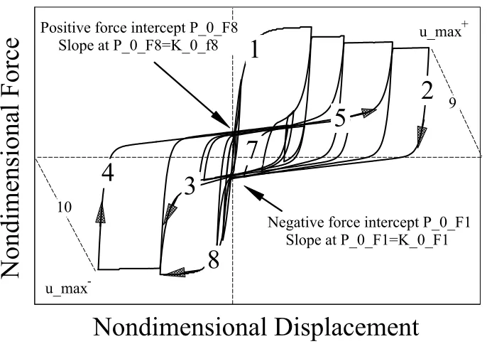
identification techniques requires three joint tests to identify the system parameters (Fig. 3).

Nondimensional Displacement

Nondimensional Force

1

5

8

7

2

4 ₃

9

10

Negative force intercept P_0_F1 Slope at P_0_F1=K_0_F1 Positive force intercept P_0_F8

Slope at P_0_F8=K_0_f8 u_max

+

u_max

(23)

The first test is monotonic to failure used to extract the backbone parameters . A nonlinear least squares approach is used to extract the data with the initial guess of



₁

provided by differentiating Eq. (0.3) for the slope of the first segment at u=0 and dividing by the maximum load recorded in the test since the min

k

eta term in the equation is small relative to the initial slope.

Mean Displacement (mm)

0 5 10 15 20 25

0.0 0.2 0.4 0.6 0.8 1.0 1.2

0 50 100 150 200 250 300 350

Static Test Time (s)

Mean Displacement (mm)

0 5 10 15 20 25

Mean L

oad

(Normalized to Maximum Static Mean)

0.0 0.2 0.4 0.6 0.8 1.0 1.2

Dynamic Test Time (s)

0.00 0.02 0.04 0.06 0.08 0.10

D 95 H D

D 95 L

S 95 H

S 95 L S

Fig. 2 Variation in monotonic tests of nailed connections (Yeh et al. 1999) (H=Upper 95 % Confidence Interval, L=Lower 95 % Confidence Interval)

Cycle 0.0 0.1 0.2 0.3 0.4 0.5 0.6 0.7 Time Displacement Cycle -3 -2 -1 0 1 2 3

(a) (b) (c)

(24)

The second test involves a zero mean cyclic test in which the reversal points, their slopes and the zero force intercepts and their respectives slopes are recorded along with the energy dissipated for the given cycle. The parameters associated with the segments as shown in Fig. 1 are matched with the corresponding data and then determined using a nonlinear least squares routine for each loop. The vector of parameters for each hysteretic loop is then weighted by the energy dissipated in the loop divided by total energy dissipated for all the matching loops pertinent to the segment. Eq. (0.6) describes this mathematically. In Eq. (0.6)

n represents the cycle for the individual loops and j=2,3,4,5. ,

* *

j Energyn j n Energyn





 (0.6)

The third test extract parameters for segments 6 and 7 from a non-zero mean cyclic test. Segment 6 while not shown in Fig. 1 is the same curve but in the third quadrant rather than the first quadrant. The parameters were again extracted using a nonlinear least squares approach but without the energy dissipation as weighting criterion. In practice this test was not conducted for the research contained in subsequent sections and thus these parameters were estimated after the rest of the parameters were determined.

This approach involves significant practical difficulty in implementing given the

0 500 1000 1500 2000 2500

0 5 10 15 20

D isplace m en t (m m )

Loa

d (

N

)

-300 0 -200 0 -100 0 0 1000 2000 3000

-15 -10 -5 0 5 10 15

D isp lacem e n t (m m )

Lo

ad (

N

(25)

inherent variability in wood connections and wooden structural assemblies. An example of this variability which investigated the monotonic response of wooden connections under dynamic loading (Yeh et al. 1999) is shown in Fig. 2. The results include thirteen tests under dynamic loading and eight for statically loaded connections. The graphs plot the variation of the mean response over the full range of deformation. This amount of variability explains why it is quite possible that the cyclic loading maximum may exceed the monotonic

maximum from single shear joint tests as shown in Fig. 4 conducted in Collins et al. (2005). In light of the limitations imposed by the three test procedure several alternatives are available. One approach is to identify the expected demand for the system under analysis and design a test that mimics this demand. An example developed recently is that used in the CUREE loading protocol (Krawinkler et al. 2001). This loading protocol simulates the demand on wood construction under seismic loading. The backbone curve and associated parameters could be estimated as in Folz and Filiatrault (2001) and more recently Pang et al. (2007) where they assume the backbone is defined by the peaks of the cyclic loops. In this case the system identification for test 2 outlined above would identify the parameters

governing the pinched loops of the hysteresis. This approach explicitly includes some of the cyclic degradation in the backbone function and thus the degradation parameter discussed later would yield a reduced value. An additional iteration would then be necessary to confirm the assumption made in determining the backbone parameters.

Another approach would be to use a mechanics based approach for wood connections such as in Foschi (2000) or a Chui and Li (2006) to generate the force displacement

relationship for a specific connection configuration. After generating the monotonic response and cyclic response from either of the methods for the selected configuration the first and second part of the above system identification routine may be used.

The final approach, commonly used to determine parameters for

(26)

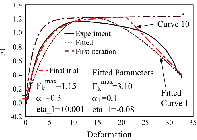
The monotonic properties are simple to extract with software capable of fitting nonlinear functions by least squares methods as long as the care is taken in selecting which portions are analyzed.

Fig. 5 pointedly illustrates the care that must be exercised in an automating the analysis of data. The fitted data provides a “solution” that is clearly not physically realistic as the fitted maximum load is three times the actual from the test. Another fit with applied constraints based on the maximums and minimums allowed in the mathematical formulation yield a much improved solution of max

,

k i

F = 1.24, ₁0.295 and eta_1 0 . The trial and

error solution used the maximum load and the initial slope for the estimate of max ,

k i

F and

1 with eta_1 0.001

  . The third trial is shown with curve 10 plotted starting at the selected breakpoint.

2.2 MODEL SEGMENTS

Deformation

0 5 10 15 20 25 30 35

F1

-0.2 0.0 0.2 0.4 0.6 0.8 1.0 1.2 1.4

Fitted Parameters

F

_kmax

=3.10



1

=0.1

eta_1=-0.08

Experiment Fitted

First iteration

Final trial

F

_kmax

=1.15



₁

=0.3

eta_1=+0.001

Curve 10

Fitted

Curve 1

(27)

2.2.1 Segment 1 and Segment 8

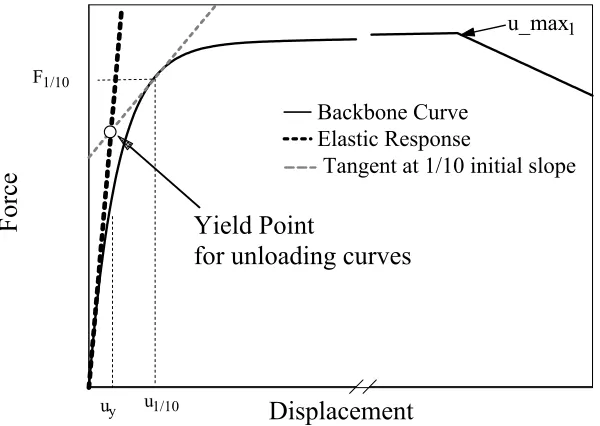
Eq. (0.3) defines the current capacity curve for the 1st and 3rd quadrants and defines the load displacement relationship when loading past the previous maximum displacement. These capacity curves, an example shown in Fig. 6, physically represent the maximum load the connection may obtain under a monotonic load. This maximum is dependent on the degradation of the load history as described in Eq. (0.5) when under non-monotonic loading. This simple degradation function calculates the maximum degraded capacity dependent on the previous load reversals. Noteworthy is the linear portion of the backbone curve in Eq. (0.3) described by the parameter eta which does not degrade with load history and is a modification from Xu (1998). The breakpoint is defined as the point of deformation, u_max1 in Fig. 6, at which the maximum load occurs after which there is a negative slope under increasing displacement.

Segment 2 and Segment 4 are described by the same functions and boundary

Displacement Force Yield Point

for unloading curves

u_max₁

Tangent at 1/10 initial slope Backbone Curve

Elastic Response

u1/10 uy F1/10

(28)

conditions in their respective positive and negative quadrants. The curve force displacement response is described by Eq. (0.4). Curve 2 operates in the 1st quadrant while curve 4 as shown in Fig. 1 defines the unloading in the 3rd quadrant. For conciseness only curve 2 will be discussed. The boundary conditions for Curve 2 are shown in Fig. 7. The reversal point, (u_r, f_r) is stored and used for calculating the degradation in positive quadrant upon the next load reversal. In Fig. 6 the defined yield point is used for calculating the zero displacement intercept, P_0_F1, for the unloading curve. P_0_F1 is found by differentiating Eq. (0.3) with respect to “u” to obtain Eq. (0.7) .

Using this equation, the initial slope is provided in Eq. (0.8) and u1/10 in Fig. 6 are

determined. In practical cases, eta_1, in Eq. (0.7) is very small compared to the initial slope and thus may be neglected leading to Eq. (0.9)

1

*

1 _max _*

1 1

* u

dF

F e eta

du



 

  (0.7)

1

max

1 1

1

(0) *

dF

F eta

du 



 (0.8)

Nondimensional Displacement

Nondimensional F

orce

7

2 (u_r,f_r)

K_0_F1 P_0_F1

(29)

1 10 1 1 ln( ) 10 u  

 (0.9)

1* 1 10

max

1 1

10 *(1 )

u

F F e (0.10)

The force at this point, ₁

10

F is calculated from Eq. (0.10) where again the eta1 term

has been neglected. The yield location is then determined by Eq. (0.11)and solving for uy

leading to (0.12).

max

1 1

1 1 1 1

10 10

*

*( ) * *

10 y y

F

F  u u  F u (0.11)

max

1 1 1

10 1 10 max 1 1 * 10 0.9* * y F u F u F    

 (0.12)

0 20 40 60

0.4 0.6 0.8 F1peak

alpha1 F1max _uy













1 xn    xn F1peak

alpha1 F1max _uy 0.5

(30)

The force intercept, P_0_F1, defined in Eq. (0.13) is a function of the previous maximum load F1(upeak) where upeak = previous maximum displacement. The exponential

term in Eq. (0.13) contains the variable xn, a counter for the number of cycles.

(1/ ) 1

1 max

1 1

( )

_ 0 _ 1 _ 8* ( )*(min( ),1)

* *

xn

y F upeak

P F s p F upeak

F u



 (0.13)

The dependence on the number of cycles for P_0_F1 is demonstrated in Fig. 8. The influence of the yield load is currently limited to load responses less than the yield load after which the ratio 1

max

1 1

( )

* * y

F upeak

F u

 >1 and the force intercept is dependent entirely on the

degraded peak force.

Segment 3 and segment 5 are described by the same functions (0.4) and boundary conditions in their respective positive and negative quadrants. Curve 3 operates in the 3rd quadrant while curve 5 defines the pinched response when loading in the 1st quadrant. Again

Nondimensional Displacement

Nondimensional Force

3

(upeak,F8 (upeak))

P_0_F1 K_0_F1

(31)

for conciseness only one will be discussed in the text. The boundary conditions for curve 3 are shown in Fig. 9. Both the peak displacement, upeak, F8(upeak) are negative and

independent of the positive peak values. F8 (peak) represents the degraded peak force at the

past negative peak displacement. The slope dF3

du at u=0 is forced to K_0_F1. The slope

K_0_F1 is calculated by Eq. (0.14)

max 1 1, _ 0 _ 1 _ 0 _ 1

_ _

i

P F

K F

f r

u r

F





 

(0.14)

where the term

max 1 1,

_

i

f r F

  represents the recoverable elastic displacement. The value of

K_0_F1 is then compared to several concavity checks of F2, F3, and initial slope on F8. If the

recoverable elastic displacement is greater than u_r then the slope is calculated by

_ 8*( _ 0 _ 1 _ ) _ 0 _ 1

_

s k P F f r

K F

u r



 (0.15)

where s_k8 is the fraction of the minimum allowed slope required for concavity in the exponential function. For small oscillations about zero this governing equation is hard numerically as it causes large changes in the calculated stiffness between loading and unloading segments. Phenomological models such as Folz and Filitrault (2001) based on Stewart’s (1987) for wood hysteretic systems have generally assumed a fixed force intercept and slope for simplicity are based often on the response of shear walls. Several models notably Takeda (1970) as well as Xu (1998) and more recently Pang et al. (2007) have again noted that the slope and intercept are not fixed and necessary for implementation in

performance based design. Pang et al. used a linear function of the previous load reversal to model the shifting intercept along with an exponential unloading function with an

(32)

Heiduscke et al. has shown that the response of a 2 story laminated frame depended on modeling the response of the densified glass fiber reinforced connections in the vicinity of the zero intercept. He also noted the incongruity in current loading protocols with the

recorded seismic rotations for a strong motion earthquake. Depending on the nature of the wood system being analyzed the loading functions may not provide sufficient information to determine a suitable load intercept model and therefore more research into the hysteretic

-800 -400 0 400 800 1200

-25 25 75 125 175 225

D isp lacem ent(m m )

For

c

e

(N)

T est 1 part1 T est1 part 2

-25 25 75 125 175 225

Displacem ent (m m )

Test 2 Model Fit

(a) (b)

-1 0 0 0 -5 0 0 0 5 0 0 1 0 0 0 1 5 0 0

-5 0 0 5 0 1 0 0 1 5 0 2 0 0 2 5 0

D is p la c e m e n t(m m )

Force(

N)

T e s t 3

-1 5 0 -5 0 D is p la c e m e n t(m m )5 0 1 5 0 2 5 0 3 5 0

S eco nd ary a m p litud e initia l C ycles T ertia ry Q u aterna ry

(c) (d)

-1 200 -800 -400 0 400 800 1 200

-1 50 -50 5 0 1 50 2 50 350 450

D is p lac em e n t(m m )

Forc

e

(N

)

(e)

(33)

response of wood systems at oscillations of varying amplitudes centered at varying displacements is needed.

Segment 6 and 7 are defined by the same equations and boundary conditions and differ only by sign. In order to gain a better understanding of the response of these hysteretic systems, a short experimental study was undertaken that examined the force intercept under non-zero mean loading. The experiment tested five reduced scale single shear dowel connections identical in their nailing configuration under a pseudo-static loading. Test one was conducted at a slower test speed (450 mm/min) for the first few cycles and the remainder of the duration of the test at 508 mm/min .

Each of the tests display the pinching, strength, stiffness degradation, and

stabilization under repeated cycles that characterize dowel bearing connections in wood. In particular the pinched response characterized by the dowel moving through previously crushed material is very evident. Comparing the experimental results in Fig. 10 and the experimental result in Fig. 11 it is clear that the reloading described by segment 7 (Fig. 1 ) as described in Xu (1998) will need the ability to match two different shapes- a “cigar shape” and the pinched response. Unfortunately the governing equation is unable to match the two shapes with a single hysteretic parameter. The solution as implemented reloads in the “cigar

Displacement

Force

Cigar shape

Pinched

(34)

shape” if the force at reversal point is greater than P_0_F8. If the force is less than the positive force intercept then the pinched response is determined and reloading again in the “cigar shape” continues to the pinched response defined by curves 3 and 5. The intersection is defined by Eq. (0.16) with the boundary conditions given in Eqs. (0.17) and (0.18). This is shown graphically in Fig. 12. A coarse example of the element response is shown in Fig. 10 (b). The model response for the loading in Fig. 11 using parameters determined from a similar specimen is shown in Fig. 13.

1

_ 0 _ 8 _

7 _

( _ _ )

_ _

i i

P F f r

u bdry u r

f r f r

u r u r



  _



(0.16)

7( 7 ) 5( 7 )

F u bdry F u bdry (0.17)

7 _{( 7} ₎ 5 _{( 7} ₎

dF dF

u bdry u bdry

du  du (0.18)

Displacement

Force

P_0_F8

(u_r _i , f_r _i)

(u_r _i-1 , f_r _i-1 )

u7bdry

F₇ = F ₅

(35)

Segment 9 and 10 are linear equations defined by the breakpoint after which increasing displacement yields a decreasing load as defined in Eq. (0.19). Eq. (0.20) identifies the point of zero remaining capacity for the system. A small residual capacity is added for numerical stability after this displacement.

9 _1*( _ max )1 1,i( _ max )1

F slope u u F u (0.19)

max

1,i 0 _{_1}

fpeak

F upeak

slope

   (0.20)

3 Hysteretic Models

A few examples of the single degree of freedom (sdof) response of the element for various types of wood structures including shear connections, moment connections, shear walls. Fig. 14 plots the displacement driven response of a single shear nail connection under several displacement patterns. The connection tests were conducted as part of the research

Displacement

Force

Experiment Model

(36)

presented in sections three, four, and five of this document. The connections were geometrically identical and loaded pseudo-statically. The loading displacements contain large displacement cycles and display asymmetric displacements about the displacement origin.

The connection parameters identified in the figure were determined from a hybrid of nonlinear least squares for estimates of the backbone parameters neglecting the eta term for curve 1 in Eq. (0.3) and trial and error for the remaining parameters for the displacement test in Fig. 14 (a). The parameters were selected to be symmetric in the positive and negative quadrants. Figures (b) through (e) plots the response of the same connection model loaded by the new displacements. The results here demonstrate the ability of the model to capture the components of the hysteresis and thus not restricting the model to specific loading sequence, e.g. zero mean cyclic test.

Displacement

-1.5 -0.5 0.5 1.5

Force -1.5 -1.0 -0.5 0.0 0.5 1.0 1.5

Kobe

Displacement

-0.5 0.5 1.5

Northridge

Displacement -2.5 -1.5 -0.5 0.5

Force -1.5 -1.0 -0.50.0 0.5 1.0 1.5

Nahinni

Displacement -2.5 -1.5 -0.5 0.5

Gazli

Displacement -2.0 -1.0 0.0 1.0 2.0

San Fernando

₁ =10

₂ =20

₁ for F8=10

₄ =-15

₅ =20

₆ =15

₇ =2.5

₈ =2.5

₁ =0.125

₈ =0.125

Fmax₁ = 1.35 s_p1=0.2 k₁min=0.3 Fmax₈ = 1.35

s_p8=0.2 k₁min=0.3

u_max+=7 u_max-=7 eta_1=0.02 eta_8=0.02

(a) (b)

(c) (d) (e)

Experiment Analytical

(37)

This section demonstrates the ability to simulate a moment resisting connection of laminated frames. Fig. 15 compares the analytical fit for quasi-static cyclic test (QSCT). If the expected displacement demands correspond to the joint test data then this match should be further refined by using the system identification outlined earlier by

weighting the vector of parameters by the energy dissipated.

The parameters determined for this match were then used examine the connection response to an arbitrary load defined by an arbitrary artificial earthquake a defined in IEEE 344 (1987) followed by the QSCT loading. The test amplitudes and loading sequence are shown in Fig. 16. The third portion of the test is the same displacement pattern scaled by 10. There is reasonable agreement among the first three tests although by the fourth test there is a clear error in the model’s ability to evaluate the response. The equation governing the

location of the zero force intercept is not capturing the shift under the reduced loading displacements. This causes an error in the dissipated energy. The next loading by the QSCT shows reasonable agreement with an error in the amount of degradation.

The next comparison in Fig. 17 and Fig. 18 displays the response of the same joint configuration but without without the glass fiber reinforcement. Again the parameters are fitted from the QSCT and then compared to the arbitrary loading. The parameters for Eq.

- 0 . 6 - 0 . 4 - 0 . 2 0 0 . 2 0 . 4 0 . 6

- 0 . 4 - 0 . 2 0 0 . 2 0 . 4

R o t a t i o n [ r a d ]

Mo

m

e

n

t [k

Nm

]

E x p e r i m e n t a l

A n a l y t i c a l

(38)

(0.3) are kept symmetric with only the zero force intercept slightly different for the positive and negative intercept. There is overcapacity predicted in. Fig. 17 The results show that the pinching function could be improved when under an increased number of cycles associated such as with the five tests of the arbitrary load.

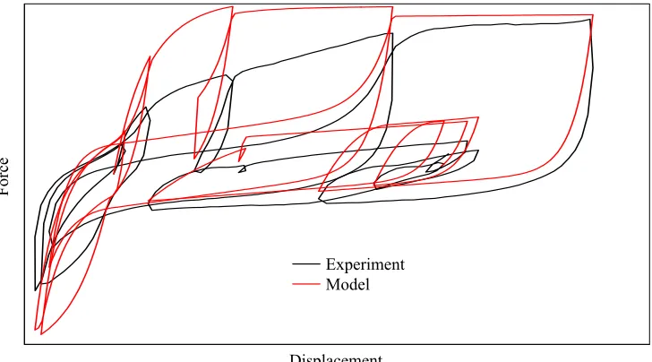
The last comparison is of a gypsum clad wall tested by Paevere et al.(2002). The sdof connection model is able to capture the shear wall hysteresis under the reversed cyclic load (ISO 2000). This standard adequately approximates the seismic demand on wood subsytems as shown in Gatto and Uang (2003). The energy dissipated under this protocol is similar to the protocol developed by Krawinkler (2001) for wood structures under seismic loading and as such could the proposed model could be expected predict the seismic demand for this substructure.

Rotation (rad)

-0.015 0.000 0.015

-0.15 0.00

0.15

Alt2

Rotation (rad)

-0.15 0.00 0.15

Moment (kNm) -0.6

0.0

0.6

Alt3

Rotation (rad)

-0.015 0.000 0.015

-0.15 0.00

0.15

Alt4

Rotation (rad)

-0.3 0.0 0.3

-0.6 0.0

0.6

QSCT

Pseudotime

0x100 2x104 3x104

Rotation (rad)

-0.3 -0.1 0.0 0.1 0.3

Loading Sequence

Rotation (rad)

-0.015 0.000 0.015

Moment (kNm)

-0.15 0.00 0.15

Alt1

Experimental Analytical Alt1

Alt2 Alt3

Alt4 QSCT

(39)

-0.4 -0.2 0 0.2 0.4

-0.40 -0.20 0.00 0.20 0.40

Rotation [rad]

Mome

nt [k

Nm]

Experimental Analytical

Fig. 17 Analytical fit of model of moment resisting joint under QSCT loading for Type III unreinforced connection

-0.5 -0.3 0.0 0.3 0.5

-0.30 -0.20 -0.10 0.00 0.10 0.20 0.30

Rotation (rad)

Mo

m

e

n

t (

k

Nm

)

Experimental Analytical

(40)

4 Conclusions

The proposed finite element formulation of hysteresis of wood connections, wood subsystems was shown to adequately match the strength and stiffness degradation, pinching, and history dependence for a variety of connections under cyclic zero mean and arbitrary cyclic tests. The parameters for the proposed formulation may be obtained through a system identification routine programmed in Matlab by a nonlinear least squares routine.

-40 -30 -20 -10 0 10 20 30 40

-125 -100 -75 -50 -25 0 25 50 75 100 125

Displacement (mm)

Forc

e

(k

N)

Experiment Model

(41)

Notation

j m

a _, = parameters calculated from curve boundary conditions for each cycle m=1,2,3

min

k

eta = Minimum slope allowed on backbone curve;

eta_1 = Minimum slope allowed on backbone curve 1 eta_8 = Minimum slope allowed on backbone curve 8 f_r = Force at load reversal

s_p8 = Percent multiplier of F upeak₁( )

min 1

k = Multiplier for K_0_F1 for allowable level of concavity

slope_1= Negative slope on curve 9

u = Element deformation;

 / max

u = Deformation at maximum peak load in quadrant 1 and 3;

u_max- = Deformation at maximum peak load,negative quadrant u_max+= Deformation at maximum peak load,positve quadrant u_r = Displacement at load reversal

1 10

u = Tangent point at 1/10 initial slope of Curve 1

y

u = Intecept of initial slope and slope at tangent of 1/10 initial slope

upeak = Maximum recorded displacement u7bdry= Boundary displacement for curve 7 xn = Number of Cycles



= Summation

n

Energy = Dissipated energy for cycle n 1

10

F = Force at tanget at 1/10 initial slope of Curve 1

 

Fe = Element Load Vector

i

(42)

R i

F = force at the load reversal of the i-th cycle;

) (u

Fj = generalized force in the element on jth curve j=2,3,..7;

) (u

F_k = generalized force in the element when loading follows backbone function; max

,i k

F = maximum degraded capacity of the element at i-th cycle for the backbone;

Fmax = maximum connection load

H = Upper 95 % Confidence Interval

 

Ke = Element Stiffness Matrix

L = Lower 95 % Confidence Interval MDOF = multiple degree of freedom; P_0_F1= Negative force intercept P_0_F8= Positive force intercept

K_0_F8= Slope at positive force intercept K_0_F1= Slope at negative force intercept NDS = National Design Specification; SDOF = single degree of freedom

Umax = positive maximum displacement j

 = exponent governing shape of force displacement function;

k

 = exponent governing shape of backbone function;

_k = degradation rate coefficients;

df

du = Differential of load displacement 1

dF

du = Derivative of Curve 1 7

dF

du = Derivative of Curve 7 5

dF

(43)

Subscripts

i = cycle number;

j,k = curve numbers j=2,3,..7; k=1,8

References

Carr, A.J. (2000). “RUAUMOKO – Inelastic Dynamic Analysis Program”, Department of Civ. Eng., Univ. of Canterbury, Christchurch, New Zealand.

Chui,Y., Ni C., and Li, Y. (1998). “Modeling Timber Moment Connection under Reversed Cyclic Loading.” J.Struct.Eng.,131(11),1757-1763.

Chui,Y., Ni C., and Jiang L. (1998). “Finite-Element Model For Nailed Wood Joints Under Reversed Cyclic Load.” J.Struct.Eng.,124(1),96-103

Collins,M., Kasal,B., Paevere,P., and Foliente,G.C. (2005).“Three-dimensional model of light-frame wood buildings.I:Experimental Investigation and Validation of Analytical Model.” J.Struct.Eng.,131(4),676–683

Dolan, J.D. (1989). “The dynamic response of timber shear walls”. PhD thesis, Univ. of British Columbia,Vancouver,BC., Canada

Dowrick,D.j. (1986). Hysteresis loops for timber structures”. Bulletin of New Zealand National Society of Earthquake Eng., 19(20):143-152.

(44)

Foliente, G.C. (1993).”Stochastic dynamic response of wood structural systems”.PhD thesis, Virginia Polytechnic Institute and State Univ., Blacksburg,Va

Folz,B., and Filiatrault,A.(2001).‘‘Cyclic analysis of wood shearwalls.’’ J.Struct.Eng., 127(4), 433–441.

Foschi, R.O. and Yao, F., and Rogerson, D. (2000). “Determining embedment response parameters from connector tests”. Proceedings, World Conference on Timber engineering, Whistler, B.C. Canada

Foschi, R.O. (2000). “Modeling the hysteretic response of mechanical connections for wood structures”. Proceedings,World Conference in Timber Engineering , Whistler, B.C. Canada.

Heiduschke, A., Kasal,B. and Haller P. (2006) Analysis of wood-composite laminated frames under dynamic loads-analytical models and model validation. Part II: frame model. Progr. in Struct. Engr Mater. 8(3):111-119.

Institute of Electrical and Electronic Engineers (IEEE), Standard 344, Recommended Practice for Seismic Qualification of Class 1E Equipment for Nuclear Power Generating Stations, IEEE, 1987.

(45)

Krawinkler, H., Parisi, F., Ibarra, L., Ayoub, A., and Medina, R. (2001).“Development of a testing protocol for woodframe structures.” CUREE Publication No. W-02, Richmond, Calif.

Matlab (2006). www.mathworks.com. Natick, MA.

Paevere, P.J., Foliente, G.C., and Kasal, B.(2003).“Load-sharing and re-distribution in a one-story wood frame building.”J.Struct.Eng.,129(9),1275–1284.

Paevere, P.J. (2002). “Full-scale testing, modelling and analysis of light-frame structures under lateral loading.” PhD thesis. University of Melbourne, Melbourne, Australia.

Pang,W.C.,Rosowsky, D.V.,Pei,S.,and van de Lindt,J.W.(2007).“Evolutionary parameter hysteretic model for wood shearwalls.”J.Struct.Eng.,133(8),1118–1129.

Polensk,A. and Schimel, B.D. (1991).”Dynamic properties of light-frame wood subsytems”. J. Struct.Eng., 117(4),1079-1095.

Powel,G.H. Drain- 2-DX User guide. Dept. of Civ. Eng. Univ. of California Berkeley,1993.

Stewart, W. G. (1987). “The seismic design of plywood sheathed shearwalls.” PhD thesis, Univ. of Canterbury, Christchurch, New Zealand.

Swanson Analysis Systems, Inc.(2008).

(46)

Wen, Y.-K. 1980. "Equivalent Linearization for Hysteretic Systems Under Random Excitation." J. of Applied Mechanics ASME 47:150-154.

Xu, H. (1998).“Analytical Modeling of Nonlinear Hysteretic Systems.” PhD thesis, North Carolina State University ,Raleigh, NC.

(47)

Dynamically loaded light-frame wood stud walls Experimental verification of an analytical model

Collins M. S., Kasal B.

(48)

Dynamically loaded light-frame wood stud walls

Experimental verification of an analytical model

ABSTRACT: Light-frame wood structures may deform well beyond the elastic limit when

loaded by dynamic forces such as earthquakes and sea wave impacts. This paper reports the results of an investigation into the response effects of structural modeling assumptions typically made in the design of light-frame wood structures. Two dimensional and three dimensional models based on previous research were developed to simulate such responses and examine the validity of such models. The models utilize the finite-element method and include options of nonlinear connection properties, elastic constitutive laws of wood

material, large deformations, contact forces, and inertial forces. The models were subjected to an estimate of the impact load imparted by a rapidly moving sea wave. To verify the models, the results of a wave-channel experiment of a full-scale wall were used wherein the wall was instrumented with reaction load cells, displacement transducers, and strain gauges on plywood sheathing and wood framing. A closed-loop hydraulic system utilizing a time varying loading function generated the wave trains. The resulting reactions, deformations, and strains were recorded as functions of time while high-speed cameras visually recorded the failure modes and wall behavior. Material tests were conducted before and after testing to record both the observed member properties and the localized section properties.

(49)

1 Introduction

Buildings located in regions defined as high hazard coastal areas prone to flooding are required by the Federal Emergency Management Agency (FEMA) to be constructed on open foundations up to the design flood elevation (FEMA, Coastal Construction Manual 2000). Structures situated on open foundations decrease the loads imparted by flooding and wave attack thus reducing the likelihood of a structural failure when compared to solid foundations below. Under the National Flood Insurance Program (NFIP), the area beneath the raised structure can be enclosed and used for storage, building access, and vehicle parking provided the enclosure is designed to “breakaway” at the design load level thus preventing excessive loads from transferring to the foundation. The walls must therefore be designed to resist moderate load levels and yet reliably fail at a larger predetermined load level. The Coastal Construction Manual (CCM) has set forth a set of prescriptive requirements based on experiments undertaken at Oregon State and analytical studies by Tung et al (1999). As an alternative to the prescriptive requirements, models like those used by Tung et al (1999) may allow the designer or engineer more flexibility in pursuing certain design considerations such as material availability or cost minimization. Safe use of analytical models requires accurate prediction of both the structural behavior and environmental loadings. Successful prediction of a breakaway wall response requires a model that captures the critical element responses governing the overall response of the wall to wave action. In this case, the critical component is the connection behavior at either the sill plate to stud connection or the sill plate to foundation connection. This research investigated the behavior of the nailed connections, developed models of breakaway walls, and compared the analytically determined behavior with the behavior observed in wave channel tests.

Keywords: Wooden structures; Nonlinear analysis; Three-dimensional models; Finite

(50)

2 Breakaway Walls

The breakaway wall investigated here is a common stud framed wall

consisting of dimension lumber with plywood sheathing and is described in detail in Tung et al (1999) and Yeh et al (1999). A typical design wall attaches to the foundations and piles through nailer plates securely attached to the foundation or floor beams. The studs are typically 39 x 89 mm members spaced 610mm apart. The sheathing can abut but not overlap the elevated horizontal beams or joists unless a separation joint is used as specified in the CCM . The sheathing may overlap and be attached to the vertical foundation members. The vertical studs are either toe nailed or end nailed to the bottom frame member identified here as a sole or sill plate. The sill plate is then attached to either a nailer plate or an unreinforced concrete floor slab or wood grade beam. The connection between the nailer plate and the foundation,if present, is made significantly stronger than the connection between the nailer plate and the wall. This design is intended to ensure that the wall separates from the nailer plates and/or stud to sill plate and is intended as the control mechanism to maintain overall structural integrity.

Breakaway walls are primarily intended to resist lateral loads such as wind and wave

(51)

forces perpendicular to the face of the sheathing. Wave action can be described by three wave types: unbroken, broken, and breaking waves (Shore Protection Manual (SPM), 1984). An unbroken wave loading was used in this investigation due to the difficulties in measuring and specifying the time and spatial pressure distribution associated with the other two wave types. Yeh et al (1999) described simplified analytical methods for the analysis of

breakaway walls subjected to breaking wave action. Of note is the determination that breaking wave action is usually the more severe environmental loading and that unbroken waves were used here only to minimize the unknowns in the loading function.

3 Wave Forces

In order to verify the behavior of breakaway wall models, the loading must be known with sufficient accuracy to separate out the error in the predicted response due to an

approximate loading function. One method of ascertaining the loading is to outfit the wall with a sufficient number of pressure taps and build a database of the spatial and temporal distribution of the wave forces on the breakaway wall subjected to the various waves. However the use of pressure sensors over the entire wall would have substantially increased the instrumentation as well as the data acquisition costs. These costs were prohibitive and as a result, only the wave heights and reactions on the breakaway wall were recorded as a

Wave Height

Time (s)

878 880 882 884 886 888 890

Force (kN)

-10 -5 0 5 10 15 20

25 1m

0

Analytical Sole Plate Experiment Sole Plate

Analytical Top Plate Experiment. Top plate

(52)

function of time to be used in determining both the response of the wall and the loading function

Having recorded the wave height as a function of time, the next task involved determining the temporal and spatial pressure distribution with the given information. The primary period of each wave train was verified from the wave height time history at the face of the wall using discrete Fourier transforms and the primary period was used in subsequent pressure calculations. In doing so, the calculation involves neglecting the contribution from the the spectrum of wave frequencies loading the wall. This approach is consistent with the approach in Yeh (1997). Furthermore, nondimensional wave parameters were examined, e.g. Ursell number, and generally found to lie outside of the delineated range for linear wave theory. However, an initial analysis and previous research (Yeh 1997) indicated that using the recorded wave height information and an approximate spatial pressure distribution for linear waves might be sufficient for the purposes of this study.

The SPM suggests that the pressure profile generated by nonbreaking wave crests or troughs located at the wall face vary nearly linearly with the wave height. This SPM model assumes a smooth rigid wall with no overtopping. This assumption of a smooth rigid wall in contrast to the actual flexible wooden wall simplifies the fluid structure interaction to one of complete or nearly complete reflection. A schematic for the two pressure profiles is given in Fig. 1. The SPM does not describe the pressure profiles between these two loading

S t ill W a t e r L e v e l

1 8 . 9 D is t a n c e

( m ) 5 . 4 8

4 . 2 7 3 . 0 5

0 0 . 9 2 . 4 4

5 . 4 8 5 1 . 2 5 8 . 5

B r e a k a w a y W a l l W a v e

B o a r d

6 5 . 8 9 5 . 1

H ig h s p e e d V id e o c a m e r a

H ig h S p e e d V id e o C a m e r a s

(53)

conditions. However, the two profiles suggest that the changing pressure may be approximated as a linear function of the wave height.

This information, combined with the wave height time history, was used to generate loading functions for the model. The pressure coefficients were initially determined using the lengths calculated from the primary period for linear waves. An iterative process then determined the magnitude of the coefficients by comparing the measured reactions with the calculated reactions under static loading and adjusting the applied analytical pressures by the calculated ratio. The specific ratios varied depending on the wave height, wave period, still water depth, and the specific time of sampling. Ratios were estimated for the each of the nine wave trains examined and were not adjusted to match the reactions at each point in time over the duration of the analysis. Thus, the reactions may or may not match the recorded reactions at a given time instant. An example is shown in Fig. 2. The recorded reactions were multiplied by 0.88 which is the ratio of the breakaway wall area to the total wall area attached to the load cells (discussed in subsequent section).

Some additional assumptions and notes involving the conversion from recorded wave heights to the applied analytical pressures are described below. To simplify the analytical loading for the entire time history of the test, the recorded wave heights at each edge of the face of the wall were averaged for the pressure calculations. Doing so introduces a

Studs 61 cm

on center

3 5 7

4 6 8 61 cm

61 cm Strain Gauges

1

2 Rosette Strain Gauge

Displacement Transducer

S12 S49 S9

S16

S7 S48

5 x 61cm

P1 P2 P3

(54)

symmetry in the loading across the face of the wall not present in the actual experiment and thus introduces a known uncertainty into the results.

As mentioned in the preceding paragraph the pressures were adjusted to apply the correct magnitude of load. Since the pressures were adjusted by ratios calculated under static loading an assessment may be made on the importance of dynamic loading assuming the spatial distribution is approximately correct and the analytical model is sufficiently accurate. Yeh(1997) and the CEM(2000) have indicated that under nonbreaking waves the loading is essentially static. This assertion will be examined in this paper for its validity. The

hydrostatic pressure on the back side of the wall was accounted for to obtain the net pressure. A wave gauge located on the backside of the wall indicated wave transmission through the wall was negligible until near failure.

4 Experiment

This investigation into the behavior of breakaway walls under the action of oscillatory wave force was part of a larger project, which included several designs of

(55)

The breakaway walls attached to a load frame erected in the wave channel. The test wall was a standard US “2x4” construction (39 x 89 mm). The studs were placed 61 cm (24 in) on center and sheathed with plywood 12.7 mm (0.5 in) thick. The stud framing was fastened with two 16d (d=4.1 mm, l=89 mm, d= diameter, l= length) nails, end nailed to the sill plate or top plate. The plywood was fastened with 8d (d=3.3 mm, l=63.5 mm) located 15.2 cm (6 in) on center around the perimeter of each sheet and 30.4 cm (12 in.) within the field of the sheet. The sill plate and top plate attached to a nailer plate, which was securely fastened to the loading frame. The plywood did not attach to the nailer plate nor overlap the nailer plate. The wall’s sill plate was overconnected as described in Yeh(1997) to the test frame to ensure that the failure would occur within the breakaway wall and not at the sill to

Table 1 Green Wave Parameters for Wave Channel Tests on Breakaway Walls Wave

run number

Period T (s)

Wave Height H (mm)

Still Water Depth ds (mm)

Wave Length

(m)

k-92 5.77 305 792 15.8

k-93 5.77 457 792 15.8

k-94 7.62 305 1402 27.8

k-95 7.62 457 1402 27.8

k-96 4.27 457 1402 15.0

k-97 2.14 457 1402 6.3

k-98 1.35 305 1402 2.8

k-99 9.55 457 1402 35.1

k-100 7.22 610 1402 27.8

Strain G auges

242.6 cm

21.6 cm _{Load cell}

61 cm

61 cm Load cell T est fram e m e m ber T o p P late

Stud

Sole P late N ailer P late

P ly w ood

Finite Element Modeling of Light Frame Wood Structures An Integrated Approach

DEDICATION

BIOGRAPHY

ACKNOWLEDGMENTS

TABLE OF CONTENTS

LIST OF TABLES

LIST OF FIGURES

Introduction

BACKGROUND

DISSERTATION ORGANIZATION

Nonlinear Hysteretic Connections

1

Background

2

Developed hysteretic element

 

 

( )

j

2 , 3 , ..7

F

u



a



a

u



a

e







2.1

SYSTEM IDENTIFICATION OF MODEL PARAMETERS

Nondimensional Displacement

Nondimensional Force

1

5

8

7

2

4

3





2.2

MODEL SEGMENTS

Deformation

F1

Fitted Parameters

F

=3.10



=0.1

eta_1=-0.08

F

=1.15



=0.3

eta_1=+0.001

Curve 10

Fitted

Curve 1















Nondimensional Displacement

Nondimensional Force

3

3

Hysteretic Models

Kobe

Northridge

Nahinni

Gazli

₃