Electrostatic Generation and Control on Textiles.

(1)

ABSTRACT

LIU, LU. Electrostatic Generation and Control on Textiles. (Under the direction of Dr. Abdel-Fattah M. Seyam and Dr. William Oxenham).

Static electricity has been a major problem for textile manufacturing as well as consumers, especially after the introduction of manmade fibers. Extensive research has been done in this field; however, there are still questions not answered, and drawbacks. For example, the accuracy of the measurement is questionable due to the manual transfer of samples to the measuring unit, the devices and procedures are complicated and the results are not reproducible.

The goal of this research was to gain a better understanding on the mechanism of static generation and dissipation and to find the effects of different parameters on electrostatic behavior of polymeric surfaces. To realize this goal, precise material handling/cleaning and testing procedures were developed and three automated devices for electrostatic measurement were used. The devices were a linear tester, a rubbing tester, and a contact tester. The description of the devices and the analysis of signal obtained are given in Chapter 4, 5, and 6. The charge generation and dissipation behaviors of different polymers were investigated and compared. The effects of different parameters, such as the rubbing speed, contact force, environmental conditions, and antistatic finishes, are analyzed, and suggestions are given to textile industries based on the studies.

In this dissertation, literatures are reviewed in Chapter 2. The objectives are given in Chapter 3. Chapters 4, 5, 6, and 7 were modified from four manuscripts, which had been submitted to journals. The overall conclusions and suggestions for future work are given in Chapter 8.

Chapter 4 discusses the electrification produced by running a yarn against a guide and it was found that charge could be effectively controlled by reducing the relative rubbing speed between two surfaces. For several applications in textile industry, it is suggested that rotating rollers would be better than fixed guides for electrostatic control.

(2)

rubbing and reaches the saturation after 2-3 cycles of rubbing PP and PTFE, while the charge reaches saturation after 40-50 cycles of rubbing nylon. This could be related to the difference of charge dissipation behavior of different polymers. The charge saturation is reached when the charge generation and dissipation are in balance. It is found that charge decays exponentially on nylon and the charge retained is about 60% or lower after 30 seconds, while, there is no decay on PP or PTFE during 30 seconds of observation.

Chapter 6 shows research on contact charging between polymeric plates. It is also shown that charge increases as the contact force increases. In addition, the tribo-electric series were found for nylon, stainless steel, PP, and PTFE by contact against each other.

Chapter 7 reports investigation in regards to contact charging and frictional charging on polymeric plates and yarns treated by antistatic finishes. It is found that ionic finish performs better than nonionic finish on both nylon and PP, and cationic finish works better than anionic finish due to difference in antistatic mechanism. From the observation of charge decay, it is found that there are two types of charge on nylon surface, which have different decay properties resulting from decay through air and spread on the surface.

(3)

Electrostatic Generation And Control on Textiles

by Lu Liu

A dissertation submitted to the Graduate Faculty of North Carolina State University

in partial fulfillment of the requirements of the Degree of

Doctor of Philosophy

Fiber and Polymer Science

Raleigh, North Carolina

2010

APPROVED BY:

_____________________________ _____________________________ Dr. Abdel-fattah Mohamed Seyam

Co-chair of Advisory Committee

Dr. William Oxenham Co-chair of Advisory Committee

_________________ _________________ __________________ Dr. Thomas Theyson

(4)

DEDICATION

Dedicated to my husband Li Yang

for his support and help in the whole process of my Ph.D. studying

(5)

BIOGRAPHY

(6)

ACKNOWLEGEMENTS

The author wishes to express her appreciation to her advisors, Dr. Abdel-fattah Mohamed Seyam and Dr. William Oxenham, for the opportunity to work on this project and their guidance throughout the whole research. The author also wants to thank Dr. Thomas Theyson, who provided the materials for this research and gave extensive suggestions. The appreciation is extended to the other committee members, Dr. Jacqueline Krim and Dr. Kristin Thoney for their advice and help.

The author would like to thank Dr. Peter Castle of Western Ontario University, Canada, for his discussion and suggestions at the beginning period of this project. The author wants to thank Dr. Yiyun Cai of USDA for training on the use of equipments. The author also would like to thank Nguyen Dzung for help in modify and updating some devices. Additionally, the author extends her thanks to her partners and officemates, Vamsi Krishna Jasti, Tamer Hamouda, and Ahamed Hassanin for their support and help.

The author is also indebted to the National Textile Center for the financial support that enables the present research to be conducted.

(7)

LIST OF TABLES

Table 1.1 Approximate value of charge potential generated in different situations (Welker, Nagarajan, &

Newberg, 2006) ... 3

Table 2.1 ESD control requirements summary ... 5

Table 2.2 Classification of materials by their resistivity (unit: ohm) ... 9

Table 2.3 Dielectric constant of materials (Dielectric Constant Reference Guide) ... 15

Table 2.4 Work functions of polymers ... 19

Table 2.5 Order of magnitude of charge density observed on various materials after contact with metals .. 20

Table 2.6 Penetration depths of charge from metal into polymers (Labadz & Lowell, 1986) ... 25

Table 2.7 Indentation characteristics of polymers(Pascoe & Tabor, 1956) ... 41

Table 2.8 Effect of relative humidity on electrostatics ... 44

Table 2.9 Optimum fiber blend for staple yarn to minimize charge ... 53

Table 2.10 Intrinsic impurities for different structures(1980) ... 55

Table 2.11 Fiber crystallinity (Morton & Hearle, 2008) ... 56

Table 2.12 Triboelectric series ... 57

Table 4.1 Experimental design-I ... 78

Table 4.2 Experimental design-II (Dpin: 25.4 mm, Vy: 100 m/min) ... 79

Table 5.1 Experimental design I used to study the effect of contact force on static generation/dissipation of polymers after rubbing against stainless steel ...108

Table 5.2Experimental design II for studying the effect of rubbing speed on static behavior of polymers after rubbing against stainless steel ...108

Table 5.3Experimental design III for investigating static properties of polymers after rubbing against each other ...108

Table 6.1 Experimental design I ...135

Table 6.2 Experimental design II used to investigate the static generation of nylon, PP, stainless steel, and PTFE by contact against each other ...136

Table 7.1 Components of model surface finishes ...149

Table 7.2 Experimental design I ...151

(11)

LIST OF FIGURES

Figure 2.1 Basic setup for surface resistivity measurement ... 8

Figure 2.2 Surface resistivity measurement configuration by concentric ring electrodes ... 9

Figure 2.3 Effect of relative humidity on resistance of yarn bundles made of different materials (temperature: 20°C) (Hearle, 1953) ... 11

Figure 2.4 Effect of temperature on resistance of cotton yarn bundles (moisture contents were calculated by weighting dry samples and samples after conditioning under the testing relative humidity) (Hearle, 1953) 12 Figure 2.5 Effect of voltage on the resistance of cotton yarn bundles (moisture content: 6.8%, R100: the resistance measured under 100 voltage) (Hearle, 1953) ... 13

Figure 2.6 Charge transfer by making and breaking contacts (Taylor & Secker, 1994) ... 16

Figure 2.7 Charges recombine (left) and remain (right) (Taylor & Secker, 1994) ... 16

Figure 2.8 Metal A and B of different work functions (b) Fermi level* of the two metals become equal after contact (Taylor & Secker, 1994) ... 17

Figure 2.9 Energy band for (a) intrinsic (b) n-type and (c) p-type semiconductor (Taylor & Secker, 1994) (Ec is energy level of conduction band, EG is energy gap between the conduction band and the valence band, Ed is energy level of donors, EF is the Fermi energy level, Ea is the every level of acceptors) ... 18

Figure 2.10 Asymmetric rubbing (Morton & Hearle, 2008) ... 22

Figure 2.11 Corona charging, Va is applied potential and Vs is the surface potential (Taylor & Secker, 1994) ... 23

Figure 2.12 Charge backflow from insulator I to metal M(Lowell & Rose-Innes, 1980) ... 28

Figure 2.13 Charge decay of a conductor characterized by its capacitance C and resistance R with respect to ground ... 30

Figure 2.14 Charge dissipation (Taylor & Secker, 1994) ... 31

Figure 2.15 Charge decay of charged insulator resting on grounded plane ... 33

Figure 2.16 Charge decay of charge insulator resting on a grounded plane with a grounded plate placed parallel with the charged surface ... 33

Figure 2.17 Charged body in air with ions ... 34

Figure 2.18 Decay curves of charge on PET film (Ieda & Shinohara, 1967) ... 35

Figure 2.19 Diagram of apparatus for measurement of electrostatic charge ... 38

Figure 2.20 Deformation of OB hard elastic (diamond), OE soft elastic, and OI polymers (The full line represents the load-deformation curves (similar to stain-stress curve), and the dotted curves are pressure-area curves under constant loads. The intersection points indicate the equilibrium situation.) ... 42

Figure 2.21 Effect of temperature on the amount of water in air (Wikipedia_Humidity)_{... 47}

Figure 2.22 Paschen curves obtained for Helium, Neon, Argon, Hydrogen and Nitrogen, using the expression for the beakdown voltage, VB as a function of the parameters pd, where, p is the pressure (torr), d is the gap distance (cm) between two parallel paltes. ... 48

Figure 2.23 Blends of nylon-Dacron polyester staple-charge developed against chrome-plated surface. .... 54

Figure 2.24 Blends of nylon-Dacron polyester staple-charge developed against cotton ... 54

Figure 4.1 Linear Tester ... 77

Figure 4.2 Yarn/pin contact angle (same contact angle for pins of two sizes), θ=60° ... 77

Figure 4.3 Force diagram analysis on the yarn section contacted with pin when Vy was smaller than Vp (left) and when Vy was larger than Vp (right)... 80

(12)

Figure 4.5 Data of figure 4.4 corresponding to the speed of charge pin ... 82 Figure 4.6 Data of figure 4.4 corresponding to the speed of yarn ... 83 Figure 4.7 Effect of yarn/pin relative rubbing speed on yarn surface potential measured by the probe-II (pin: stainless steel cylinder of 25.4 mm diameter, yarn: 420/72 nylon multifilament with anionic lubricant) ... 83 Figure 4.8 Effect of yarn/pin relative rubbing speed on yarn output tension (pin: stainless steel cylinder of 25.4 mm diameter, yarn: 420/72 nylon multifilament with anionic lubricant) ... 84 Figure 4.9 Effect of yarn/pin relative rubbing speed on contact force on yarn (pin: stainless steel cylinder of 25.4 mm diameter, yarn: 420/72 nylon multifilament with anionic lubricant) ... 85 Figure 4.10 Effect of yarn/pin relative rubbing speed on friction force on yarn (pin: stainless steel cylinder of 25.4 mm diameter, yarn: 420/72 nylon multifilament with anionic lubricant) ... 85 Figure 4.11 Effect of yarn/pin relative rubbing speed on yarn/pin coefficient of friction (pin: stainless steel cylinder of 25.4 mm diameter, yarn: 420/72 nylon multifilament with anionic lubricant) ... 86 Figure 4.12 Correlation between yarn potential-I and yarn/pin friction force (pin: stainless steel cylinder of 25.4 mm diameter, yarn: 420/72 nylon multifilament with anionic lubricant) ... 86 Figure 4.13 Pin vibration amplitude measured at different rotating frequency (pin: stainless steel cylinder of 25.4 mm diameter, yarn: 420/72 nylon multifilament with anionic lubricant) ... 87 Figure 4.14 Vibration force calculated at different yarn/pin speeds (pin: stainless steel cylinder of 25.4 mm diameter, yarn: 420/72 nylon multifilament with anionic lubricant) ... 88 Figure 4.15 Effect of yarn/pin relative rubbing speed on yarn surface potential measured by the probe-I (pin: stainless steel cylinder of 6.35 mm diameter, yarn: 420/72 nylon multifilament with anionic lubricant) ... 89 Figure 4.16 Effect of yarn/pin relative rubbing speed on yarn surface potential measured by the probe-II (pin: stainless steel cylinder of 6.35 mm diameter, yarn: 420/72 nylon multifilament with anionic lubricant) ... 89 Figure 4.17 Effect of probe-I to pin spacing (the spacing from the aperture of probe-I to the yarn/pin separation point) on measured yarn potential (the position of probe-II was fixed) (yarn: nylon with lubricant, pin: stainless steel cylinder of 25.4 mm diameter; Vy = 100 m/min, Vp = 0, input tension=50 cN) ... 90 Figure 4.18 Effect of yarn/pin relative rubbing speed on yarn output tension (pin: stainless steel cylinder of 6.35 mm diameter, yarn: 420/72 nylon multifilament with anionic lubricant) ... 91 Figure 4.19. Effect of yarn/pin relative rubbing speed on yarn/pin contact force (pin: stainless steel cylinder of 6.35 mm diameter, yarn: 420/72 nylon multifilament with anionic lubricant) ... 92 Figure 4.20 Effect of yarn/pin relative rubbing speed on yarn/pin friction force (pin: stainless steel cylinder of 6.35 mm diameter, yarn: 420/72 nylon multifilament with anionic lubricant) ... 92 Figure 4.21 Effect of yarn/pin relative rubbing speed on yarn/pin coefficient of friction (pin: stainless steel cylinder of 6.35 mm diameter, yarn: 420/72 nylon multifilament with anionic lubricant) ... 93 Figure 4.22 Effect of yarn/pin relative rubbing speed on finish free yarns’ surface charge potential

measured by the first probe (pin: stainless steel cylinder of 25.4mm diameter) ... 94 Figure 4.23 Effect of yarn/pin relative rubbing speed on finish free yarns’ surface charge potential

(13)

Figure 4.27 Effect of yarn/pin relative rubbing speed on yarn/pin coefficient of friction (pin: stainless steel

cylinder of 25.4mm diameter) ... 97

Figure 4.28 . Charge potential-I on finish free yarns corresponding to the yarn/pin friction force ... 97

Figure 5.1 Rubbing tester ...105

Figure 5.2 Charge potential on nylon in terms of time and locations of potential probe, rubbing head, and rubbing area at starting point (t = 0) and at reversing point (t = 1.2 second) in the first cycle ...110

Figure 5.3Charge accumulations in 50 cycles and charge decay on nylon surface ...111

Figure 5.4Charge accumulations in 50 cycles and charge decay on PTFE surface ...112

Figure 5.5Charge accumulations in 50 cycles and charge decay on PP surface ...112

Figure 5.6Effect of contact force on charge generated on polymer surfaces after the first cycle of rubbing against stainless steel (rubbing speed: 27 mm/sec) ...114

Figure 5.7 Effect of contact force on charge accumulated on polymer surfaces after 50 cycles of rubbing/contact against stainless steel (rubbing speed: 27 mm/sec) ...114

Figure 5.8 Effect of contact force on charge retained on polymer surfaces after 30 seconds of decay time ...115

Figure 5.9 Effect of contact force on normalized charge retained on polymer surfaces after 30 seconds of decay time...115

Figure 5.10Charge potential of the first and second cycles of rubbing (contact force: 1N, rubbing speed: 47 mm/sec) ...116

Figure 5.11Exponential behavior of charge decay of nylon ...117

Figure 5.12Charge decay model of a charged polymeric rubbing plate ...118

Figure 5.13Effect of rubbing speed on charge generated on polymeric surface after the first cycle of rubbing or the first contact/separation against stainless steel ...120

Figure 5.14Effect of rubbing speed on charge generated on polymeric surface after 50 cycles of rubbing (99 strokes) or 99 contacts/separations against stainless steel ...120

Figure 5.15Effect of rubbing speed on charge retained on polymeric surfaces after 30 seconds of decay 121 Figure 5.16Effect of rubbing speed on normalized charge retained on polymeric surfaces after 30 seconds of decay ...121

Figure 5.17Triboelectric series of nylon, stainless steel, PP, and PTFE ...122

Figure 5.18Charge potential on rubbing plate after the first cycle of rubbing against the rubbing head (rubbing speed: 47 mm/sec, contact force: 1N) ...123

Figure 5.19Charge potential on rubbing plate after 50 cycles of rubbing against the rubbing head (rubbing speed: 47 mm/sec, contact force: 1N) ...124

Figure 6.1 A Diagram of the contact charge generation/dissipation measurement device ...130

Figure 6.2Image of the contact device ...130

Figure 6.3 Typical static charge data of repeated contact test ...131

Figure 6.4Electrostatic charges of 50 cycles of contact ...133

Figure 6.5 Experimental data of Figure 6.4 and derived exponential regression relationship of charge generated in terms of cycle number ...133

Figure 6.6 Images and dimensions of contact heads ...135

Figure 6.7 Charge generated on PTFE after the first contact against nylon ...137

Figure 6.8 Charge generated on PTFE after 50 cycles of contacts against nylon ...138

Figure 6.11 Charge generated on PTFE by repeated contacts/separations against nylon, at different contact force (temperature of 30°C and R. H. of 30%) ...139

(14)

Figure 6.13 Data of Figure 6.9 sorted by the temperature ...140 Figure 6.14 Charge generated on PP after 50 cycles of contacts against nylon, stainless steel, and PTFE ...142 Figure 6.15 Charge generated on PTFE after 50 cycles of contacts against nylon, stainless steel, and PP 143 Figure 7.1 Schematic of surface treatment by an air brush ...150 Figure 7.2 Charge generated on PP after the first contact against stainless steel ...153

Figure 7.3 Charge generated on PP after 50 contacts/separations against stainless steel ...153 Figure 7.4 Surface charge potential of nylon after the first cycle and 50 cycles of rubbing against stainless

steel ...154 Figure 7.5Experimental data of charge decay of blank nylon and nylon treated by nonionic finish after 50 cycles of rubbing against stainless steel and regression curves ...156 Figure 7.6Experimental data of charge decay on blank nylon and the regression curves ...156 Figure 7.7Experimental data of charge decay on nylon treated by 0.025% nonionic solution and the regression curves ...157 Figure 7.8Experimental data of charge decay on nylon treated by 0.05% nonionic solution and the

regression curves ...157 Figure 7.9Surface charge potential of nylon yarns by moving over a chrome pin (surface concentration of active finish: 7 mg/m2_{, nylon yarns: 200 denier/60 filaments, yarn speed: 300 m/min, yarn input tension: 20}

(15)

1 INTRODUCTION

(16)

Static charge has positive and negative attributes. On one hand, it is useful in electrets filters and the formation of textiles structures such as electro-spinning and flocking. On the other hand, it has negative impacts on processes and products. For example, charge accumulation during the processing of yarns, fabrics, or films may cause irregularity of textiles and low efficiency of manufacturing. Major issues to end users are related to static generation and discharge such as clinging of clothes and discomfort from static shock when walking on a carpet and touching a doorknob. More seriously, potential life threatening accidents may take place because of static generation and discharge such as initiation of major fires at gas stations and failure of a parachute to open. Table 1.1 shows the approximate levels of charge potential generated in different situations.

To minimize the impact of static electrification, it is necessary to obtain a better understanding of the mechanisms involved in static generation and dissipation. Electrostatic charge is generated by contact and separating two different surfaces (contact charging). When two different surfaces were contacted, charge would transfer from surface of high Fermi level to surface of low Femi level. When the two surfaces are separated, the transferred charge would be recombined (metals contact/separation) or be trapped on the surface (insulators contact/separation), which is determined by the static properties of contacted surfaces. Charge generated by rubbing two surfaces (frictional charging) is more severe than the contact charging, which is more complex. It could be affected by the rubbing speed and local temperature of the surface. The mechanisms of electrostatics will be reviewed in section 2.3 and 2.4.

(17)

reading would be very different. Extensive research has been done in this field, which is reviewed in section 2.5. However, there are still questions, and drawbacks. For example, the accuracy of the measurement is questionable due to manual transfer of sample to the measuring unit, the devices and procedures are complicated and the results are not producible. Therefore, a more critical study is required on the electrostatics in textiles.

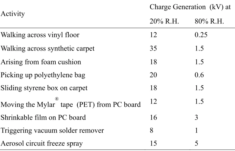
Table 1.1 Approximate value of charge potential generated in different situations (Welker, Nagarajan, & Newberg, 2006)

Activity Charge Generation (kV) at

20% R.H. 80% R.H.

Walking across vinyl floor 12 0.25

Walking across synthetic carpet 35 1.5

Arising from foam cushion 18 1.5

Picking up polyethylene bag 20 0.6

Sliding styrene box on carpet 18 1.5

Moving the Mylar® tape (PET) from PC board 12 1.5

Shrinkable film on PC board 16 3

Triggering vacuum solder remover 8 1

(18)

(19)

2.1 Electrostatic regulations

Worldwide, there are almost one hundred standards and testing methods associated with static generation and dissipation (1999). They are published by institutes such as:

 U.S. Military Department of Defense (DOD)

 American Society for Testing and Materials (ASTM)

 National Fire Protection Association (NFPA)

 Joint Electron Device Engineering Council (JEDEC)

 International Electro technical Commission (IEC)

 American National Standards Institute (ANSI)

 Institute of Electrical and Electronics Engineers (IEEE)

 Electronic Industries Alliance (EIA)

 ESD Association (ESDA)

Generally, the electrical resistance of an item is used alone or combined with the charge potential generated on the item to evaluate its electrostatic properties, though it is still questionable whether the resistance is necessarily correlated with the static generation or dissipation (Owen, 1990). Table 2.1 shows static control levels (as inferred from resistance) recommended by several standards. The testing methods are described in detail inside the standard.

Table 2.1 ESD control requirements summary

ESD Control Item Recommended Range Standard

Work surface _<1x109_{ohm and/or <200 Volts ESD S 4.1}

Wrist Strap Cord _0.8x106_{to 1.2x10}6_ohm ESD S 1.1

Footwear _<1x109_ohm ESD S 9.1

Flooring _<1x109_ohm ANSI ESD S 7.1

(20)

The charge potential generated on an item is also used for qualifying its electrostatic properties. For example, the Military Standard 883 classifies items as

follows using the standard 100 pF, 1.5 KΩ human body model:

 Class 1: > 0 to ≤ 1999 V

 Class 2: > 2000 to ≤ 3999 V

 Class 3: > 4000 V and above

In industry, to evaluate whether a work area is safe from potential static hazards, the working areas are classified into three different levels characterized by the discharge time and the charge potential (Welker, Nagarajan, & Newberg, 2006):

 For critical ESD (electrostatic discharge) safe work areas, the float potential

should be less than ± 20 V and the discharge time should be less than 20 seconds from ± 1000 V to less than ± 20 V.

 For highly sensitive but not critical ESD-safe work areas, the float potential

should be less than ± 50 V and the discharge time should be less than 20 seconds from ± 1000 V to less than ± 50 V.

 For conventional ESD-safe work areas, the float potential should be less than ±

100 V, and the discharge time can be less than 45 seconds from ± 1000 V to less than ± 100 V.

(21)

Charge generation varies widely with the moisture content of a material. The conditioning time required depends on the rate of adsorption of moisture and the

thickness (or mass) of the specimen. Thick sheets, for example, it takes a much longer

time to condition then thin films. For another example, materials with high affinity (or

absorptive capacity) for water take longer to condition than those with low affinity.Since

there is a hysteresis effect on conditioning of many materials, the moisture content of a specimen also depends on whether the material was wetter or dryer than the conditions of the test. It is required by ATMS 4470-97 that the specimens should be dryer than the specified test condition before conditioning and the specimens should be equally conditioned for at least 24 hours at the specified relative humidity before testing. Additionally, not only it is important to condition specimens properly at the required relative humilities prior to the test, but the test should also be conducted in the same conditioning environment.

Practical considerations favor conditioning in the following two environments: (1) preferably 20±2% relative humidity, 23±2°C, (2) preferably 50±2% relative humidity, 23±2°C. Other relative humidity may be adopted depending on specific end-use requirements. However, the relative humidity, temperatures, and the conditioning time are required to clearly state in the test results.

2.2 Electrostatic related characteristics - resistivity and capacitance

The resistivity and capacitance are important electrical characterizations of materials. Their definitions, testing methods, and how they are affected by other factors, like the relative humidity and temperature, are reviewed in this part.

2.2.1 Surface resistance/resistivity

(22)

which is mostly determined by surface properties of materials, thus the surface resistance, instead of the volume resistance, is usually more important in studies of electrostatic.

Concepts of surface resistance and surface resistivity can be sometimes confusing. Definitions of both terms can be found in many book and standards. Surface resistance,

RS, is defined as the ratio of a DC voltage U to the current, Is flowing between two

electrodes of specified configuration (Figure 2.1) that are in contact with the same side of

a material. The surface resistivity, ρs is determined by the ratio of DC voltage U drop per

unit length L to the surface current Is per unit width D (equation [1-1]). The surface

resistivity is the intrinsic property of a surface, which is not affected by the measured

surface area. The physical unit of surface resistivity is also ohm (Ω). In order to

differentiate from the volume resistivity, the surface resistivity is expressed also in

ohm/square (Ω/square).

Figure 2.1 Basic setup for surface resistivity measurement

(23)

the electrodes. The electrical current flows from the inter electrode to the outer electrode through the sample surface.

Figure 2.2 Surface resistivity measurement configuration by concentric ring electrodes

The resistance was used by standards to evaluate static properties of items as shown in Table 2.1. Furthermore, the surface resistivity and the linear resistivity (volume resistance per unit length, ohm/m) are often used to classify materials of isolative, antistatic, static dissipative, conductive, etc, as shown in Table 2.2. The term “static dissipative” is not synonymous with the term “antistatic”. The "static dissipative material" defines material on which charge can decay quickly, while the material's charge generation ability is not concerned. On the other hand, the "antistatic material" represents material that resists charging and produces minimal static charge generation.

Table 2.2 Classification of materials by their resistivity (unit: ohm)

Classification ESDA Standards Typical Vendor Kanarek & Tan (1998)

Isolative ND1 ND ND

Antistatic ND 1010-1014 Ω/sq ND

Static dissipative 10

2

-109Ω/m

105-1012Ω/sq 10

2

-108Ω/sq 10

5

-1012Ω/m

105-1012Ω/sq

Resistive ND ND ND

(24)

<105Ω/sq <105Ω/sq

Electrostatic shielding ND ND _<10Ω/m

EMI shielding ND ₁₀-2_-1.0Ω/sq ND

1_{ND: not defined}

Besides the resistivity of materials, the conductivity is sometimes used to describe material electrical properties, which is the reciprocal of surface resistivity.

2.2.2 Questions related to the resistivity of polymers

There are mainly three questions raised from the literature review of surface resistivity of polymers.

1) Does the volume resistivity affect the surface resistivity?

Using the standard surface resistivity testing method, the electrical current will flow mostly along the surface, thus the surface conducting mechanism was dominant. However, the measurement of surface resistivity is affected by the volume resistivity (Taylor & Secker, 1994). For example, the charge conduction of fibers depends on the contacts between fibers surface as well as the fibers bulk, which is hard to separate.

2) Are the effects of different factors on the resistivity of polymers the same as that

on the resistivity of conductors?

The resistivity of conductors has been well understood, for example, the resistivity of metals decreased as the temperature increased. However, the effects of different factors on the resistivity of polymers are not always the same as that for conductors. It is pointed out in the ASTM D257 that the resistance of insulators decreases both with increasing temperature and with increasing humidity. In addition, for polymers, the volume resistance is particularly sensitive to temperature changes, while surface resistance changes greatly and very rapidly with humidity changes.

(25)

a) The effect of relative humidity

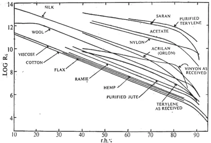
Testing environments of different levels of relative humidity were realized using saturated solutions of different salts inside testing jars. The results are shown in Figure 2.3, which indicates that the resistance of yarn bundles decreases as the relative humidity increases. This effect was explained as that the movement of ions and the dissociation are varying with the moisture content (Hearle, 1953).

Figure 2.3 Effect of relative humidity on resistance of yarn bundles made of different

materials (temperature: 20°C) (Hearle, 1953)

b) The effect of temperature

(26)

Figure 2.4 Effect of temperature on resistance of cotton yarn bundles (moisture contents were calculated by weighting dry samples and samples after conditioning under the

testing relative humidity)(Hearle, 1953)

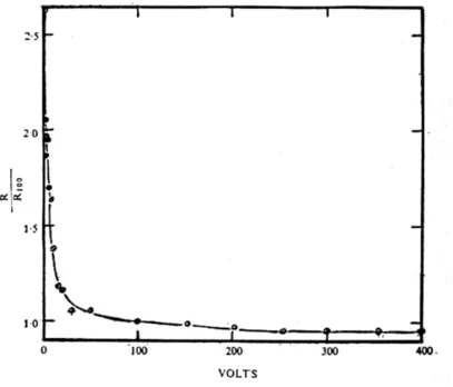
c) The effect of voltage

(27)

Figure 2.5 Effect of voltage on the resistance of cotton yarn bundles (moisture content:

6.8%, R100: the resistance measured under 100 voltage) (Hearle, 1953)

d) The effect of the tension on the specimen

The effect of tension on the yarn resistance was investigated by hanging weights on two ends of the yarn bundles. For cotton, there was a tendency for the resistance to increase as the tension is increased, but for viscose rayon filament, the resistance decreases as the tension is increased. In both case, the change was very small.

(28)

It is questionable that the surface resistivity may not necessarily correlate with the static phenomenon of the surface (Owen, 1990) and this need to be verified by further investigations.

On one hand, the mechanism of charge generation indicates that the amount of charge generated is determined by the difference of Fermi energy level of two contacted surfaces. There is no indication that surface resistivity is directly correlated to the charge generation. On the other hand, it is commonly considered that the charge decay would be affected by the surface resistivity, since the definition of surface resistivity is the resistance to the flow of electrical current across a surface. However, when the surface is not put between two electrodes, which is the setup of surface resistivity measurement, then the charge dissipation may be determined by the dielectric constant and the resistivity of the surrounding items, such as the atmosphere air and solids close to the surface (Niels, 1998).

2.2.3 Capacitance

The capacitance quantifies the ability of a system to store charge (Cardona, 2001). Its unit is Faraday, which is one coulomb per volt. If a charge is transferred from one surface to another, it produces a potential difference between them, then the capacitance of the system C can be given by equation [1-2]. For a parallel-plates capacitor, if the potential of the lower plate is zero, the system’s capacitance can be given by equation [1-3].

/ [1-2]

/ [1-3]

where q is the charge (Coulomb), C is the system capacitance (Faraday), V is the

potential (Volt), ε0 is the vacuum permittivity, ε is the media permittivity (relative

dielectric constant), A is the surface area of the plates (m2), d is the plates’ separation (m)

between plates.

(29)

dielectric constants of materials used in this work are shown in Table 2.3. The charge dissipation may be affected by the relative dielectric constant of materials (Niels, 1998), which will be discussed in detail in section 2.4.

Table 2.3 Dielectric constant of materials (Dielectric Constant Reference Guide) Medium: Vacuum Atmosphere Cotton Teflon PP PET Nylon

ε: 1 1.00054 1.3-1.4 2.1 2.25 2.8-4.5 4-5

2.3 Mechanisms of charge generation

Charge generation can be classified into contact charging, frictional charging, and corona charging according to the mode of charge generation. The contact charging or frictional charging is composed of bond-forming and bond-breaking processes and charge is generated by contacting (bond forming) and breaking (bond breaking) two different surfaces. The bond-forming process is usually explained based on an electrons-transfer mechanism; however, it is also explained by an ions-transfer mechanism. The bond-breaking process can be combined with several complicated phenomenon, such as the back-flow and gaseous discharge. In addition, charge can accumulate by repeating contacts and separations. The mechanisms on all these aspects are reviewed and discussed in this section.

2.3.1 Contact charging

(30)

which will remain on the surface and generate static (Figure 2.7). Therefore, static electricity is defined as the behavior of electric charges that rest on insulators or isolated conductors.

Figure 2.6 Charge transfer by making and breaking contacts (Taylor & Secker, 1994)

Figure 2.7 Charges recombine (left) and remain (right) (Taylor & Secker, 1994)

It is generally assumed that contact charges can be ignored for metals used in common industrial process because of charge backflow on separation. However, a series of experiments showed that charge did exist on metal balls rolling out of a metal tube into a Faraday tube Castle (2004). The possible hazards and the reason why it was not widely observed were analyzed.

(31)

against insulator) and insulator/insulator case (charging by insulator contacting against insulator) remained unsatisfactory since the lack of knowledge on insulators’ surfaces.

The theory of contact charging between metals was established in by Harper

(1957). As shown in Figure 2.8, metal A has work function φA, and metal B has work

function

φ

B, where φA <

φ

B (the work function represents the minimum energy for an

electron to escape from the metal). When the metal A and the metal B get into contact, electrons in higher energy state in metal A will transfer into unoccupied lower energy states in metal B until the surface potential is sufficient to cause the same work function for both surfaces (Taylor & Secker, 1994). The work functions of 94 elements can be found in literature (Welker, Nagarajan, & Newberg, 2006). The surface work function of most metal is about 4-5 eV.

Figure 2.8 Metal A and B of different work functions (b) Fermi level* of the two metals become equal after contact (Taylor & Secker, 1994)

*In Quantum mechanism, solid surface is occupied by electrons in discrete energy states. For metals, electrons only occupied the states below Fermi energy, EF. The energy interval, φW, from EF to vacuum

level (zero potential state) is the work function (Patterson & Bailey, 2007).

The surface energy states for semiconductor is similar to that for metal surface,

but there exists a forbidden band, EG, between the valence band and the conduction band

(32)

when they are excited, for example by thermal or optical excitation, then the electrons in the valence may jump across the forbidden band to the conduction band and the surface becomes conductive.

Intrinsic semiconductors are hard to be exited. Usually, the conductivity of semiconductors is caused by chemical impurities on their surface. Two models of semiconductors’ surface were established based on the type of the impurities: “n-type semiconductor” and “p-type semiconductor” (Figure 2.9). For the “n-type

semiconductor”, which has impurities like phosphorus (Pi) or arsenic (Se), the atoms of

impurities provide donor sites centers below the conduction band. The electrons of these atoms can be thermally excited into the conduction band easier then the electrons from the valence band, therefore contribute to the conduction. For the “p-type semiconductor”, which is caused by impurities like boron (B), the impurities atoms can generate acceptors just above the valence band. Therefore, the electrons from the valence band can be thermally excited to these acceptor atoms easier, leaving charge holes unoccupied on the valence band, which contribute to the conduction (Taylor & Secker, 1994).

Figure 2.9 Energy band for (a) intrinsic (b) n-type and (c) p-type semiconductor (Taylor

& Secker, 1994) (Ec is energy level of conduction band, EG is energy gap between the

conduction band and the valence band, Ed is energy level of donors, EF is the Fermi

(33)

Insulators can be considered as semiconductors with wide forbidden energy gap, which is too difficult for electrons to escape. The surface work functions of a range of polymers are given below (Davies, 1978):

Table 2.4 Work functions of polymers

Polymer Fermi energy (eV)

Polyvinylchloride 4.85

Polyimide 4.36 Polytetrafluoroethylene (PTFE) 4.26

Polycarbonate 4.26 Polyethyleneterephthalate 4.25

Polystyrene 4.22

Nylon 66 4.08

Based on the electronic-transfer theory, Cowley and Sze (1965) first gave an expression to calculate the charge transferred in metal/semiconductor contact, which is

proportional to the different of surface work function, φA -

φ

B. The calculating method

was improved by Hays and Donald (1971), Krupp (1971), Bauser et al (1974), Davies (1970) (1967), and Hays (1974). In addition, it was pointed out that the charge transferred

was proportional to (φA -

φ

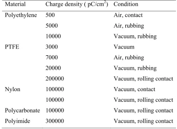
B)1/2 (Chowdry & Westgate, 1974). However, usually, the

(34)

Lowell and Rose-Innes (1980) reviewed the charge observed on various polymers after contacting with metals (Table 2.5). It is meaningless to compare the charge generated in different tests, since the real contact area could be different for different materials under different conditions. Lowell and Rose-Innes (1980) assumed that the real contact area is about half of the appearance contact area (geometric contact area), however, this is questionable and the real contact between two contacted surfaces is hard to be measured.

Table 2.5 Order of magnitude of charge density observed on various materials after contact with metals

Material Charge density ( pC/cm2) Condition

Polyethylene 500 Air, contact

5000 Air, rubbing

10000 Vacuum, rubbing

PTFE 3000 Vacuum

7000 Air, rubbing

20000 Vacuum, rubbing

200000 Vacuum, rolling contact

Nylon 100000 Vacuum, contact

100000 Vacuum, rolling contact

Polycarbonate 100000 Vacuum, rolling contact

Polyimide 300000 Vacuum, rolling contact

2.3.2 Frictional charging

(35)

(Howell, Mieszkis, & Tabor, 1959) (Gupta, 2007). As to the complex effect of speed on friction, it was found for example, that for lubricated yarns, the coefficient of friction increased when the rubbing speed increased. This is a practical example of the added complication introduced by additives (essentially deliberately applied “impurities”) which mean that some consideration must also be given to the influence of hydrodynamic factors (Lyne, 1955). Additionally, it is also interesting to note that friction could be reduced by modulating vibration (Armstrong-Helouvry, 1991), which is a factor that is of significance in a moving thread line. For those approaches that are applied to reduce friction, the ultimate goal is usually to control the electrostatic charging and reduce wear or surface attrition of the various component surfaces. While there is much work on friction and on static electrification, the correlation between these is still not well understood.

A commonly asked question is that whether rubbing charges different from charging by contact/separation. Experiments showed that charge transferred in a rubbing process was several orders of magnitude greater than in a simple contact, and it was easier for the frictional charging to reach the thermodynamic equilibrium than the repeating contact charging (Taylor & Secker, 1994). Experiments using the Van de Graff generator (Serway & Jewett, 2007) showed that charge increased as the rubbing speed (belt winding across rollers) increased. An obvious explanation of this phenomenon is that the sample length increased at higher rubbing speed, which gave more contact area for the charge generation. However, if the sample length was the same, the effect of rubbing speed on the charge generation is still unknown. It is also unknown that whether there is any more fundamental difference between rubbing charging and contact charging. If the process of rubbing were to influence the basic mechanism of charge transfer, in addition to the factor of contacting area, one would expect the velocity of rubbing to affect the charge (Lowell & Rose-Innes, 1980).

(36)

probably not important for his samples. Ohara (1980) reported that the charge transferred to a polymer by a metal sliding on it increased at first with the speed of sliding, then decreased again at high speeds, in another word, there was a certain speed at which the transferred charge was maximum. He suggested that the peak is a consequence of thermal motion of the polymer segments (details introduced in following paragraphs). Zimmer (1970) found charge reversal phenomenon (charge polarity changed) when the rubbing speed increased. They proposed that as the high speed rubbing process caused the local temperature increased, therefore enhanced the diffusion of the electrons from the hotter part to the cooler part of the surface. However, there was no method to monitor the electrons diffusion on polymers surfaces. Cunningham showed that the electrification of a polymer sheet passing over a metal roller was much greater when slipping occurred than when the roller and the polymer sheet had the same velocity. However, it could be argued that the slipping merely increases the total area of contact. A variation of this kind has been reported several times (Hersh & Montgomery, 1956) (Lowell & Rose-Innes, 1980), but it is not certain whether it was caused by back-flow of charge or whether a more fundamental process was taking effect. More works will be reviewed in details in section 2.5.

In addition, usually, charge only transfers between two different surfaces, which have different surface work functions, however, in the frictional charging, if it is asymmetric rubbing (Figure 2.10), then charge could occur on surfaces of the same material (Morton & Hearle, 2008). This is because the asymmetric rubbing generates unequal heating on the two surfaces and therefore mobile particles will move from hot to cold, owing to the greater energy of the hot particles.

(37)

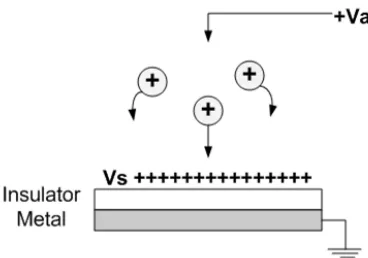
2.3.3 Corona charging

Because the charge generation in the contact and rubbing processes are hard to control, (they are sensitive to the processing parameters, such as the contact pressure and the rubbing speed) corona charging is used for observing static behavior. As shown in Figure 2.11, the corona charging is a self-sustaining, partial breakdown of gas, which is subjected to highly divergent electric field (Taylor & Secker, 1994). It is often initiated deliberately for some application, such as for the precipitation of dust and smoke and for dry powder coating. There is significant information about the corona charging (Baum,

Lewis, & Toomer, 1977)(Gas Gupta & Doughty, 1978) (Pethig, 1983). There is also

research comparing the tribocharging and the corona charging (Chubb, 2002). However, corona charging is beyond the scope of this research work.

Figure 2.11 Corona charging, Va is applied potential and Vs is the surface potential

(Taylor & Secker, 1994)

2.3.4 Repeating contacts and separations

(38)

Previous researches on the contact electrification indicated that charge increased as the number of contact increased. The rate of increase of the charge decreased as contacts were repeated, and after many contacts, the charge appeared to saturate (Lowell and Rose-Innes, 1980). Why this happens is not, however, understood. Several explanations have been put forward, as discussed below, but each of these is applicable to only a certain kind of insulator:

1) The increase of charge with increased number of contacts may be explained by the suggestion that the charge transferred depends on the total time of contact.

This simple explanation is probably not generally correct. First, charge transfer seems to occur very quickly, in a period less than the duration of individual contact in most experiments (Lowell & Rose-Innes, 1980). Secondly, specific experiments on KCl, anthracene, and some polymers (Lowell & Rose-Innes, 1980) have shown that the increase in charge by repeating contacts cannot be explained in this way. In each case, N times of contacts, each of which had t seconds of contact, generated much more charge than a single contact with contact time of N × t seconds.

2) The increase of charge with number of contacts may be caused by the increase of real contact area, which is related to the visco-elastic deformation, by repeating contacts.

(39)

3) The repeating contacts may be expected to increase the charge if the insulator is slightly conducting, because the charge tends to spread (under its own Coulomb repulsion) into the bulk, making room, for more charge to be deposited in the next contact (Harper, 1967).

Homewood and Rose-Innes (1982) used very hard crystalline insulators to study the charge accumulation, so that the surface relocation and the surface deformation in repeating contacts could be negligible. They found the charge accumulation began to happen after they added some additive to increase the surface conductivity. Therefore, they concluded that the charge accumulation was related to the surface conductivity. Between contacts, charge could leak from the contact point and be replaces on the next charging. Cunningham and Goodings (1986) observed charge accumulation a long time after the possible effect of plastic deformation has been eliminated. They assumed that the charge could penetration into the bulk, which depended on the surfaces boundary

conditions. Other reserachers (Hays, 1991) (Lowell, 1984) (Labadz & Lowell, 1986)

(Fabish & Duke, 1977) studied how charge is accumulated on an insulator and how deep the charge could penetrate. Their experiments indicated the repeating metal-polymer contact charging may involve the bulk states of the polymer, and they reported that the penetration depth is in micrometer range as shown in Table 2.6. In addition, Lowell (1967) pointed out that the charge penetration into the bulk of an insulator is caused by the thermal activation in the conduction band.

Table 2.6 Penetration depths of charge from metal into polymers (Labadz & Lowell, 1986)

Polymer Penetration depth (nm)

Polyvinyl Chloride (PVC) 48

(40)

PTFE 13 Polyethylene Terephthalate (PET) 24

Polystyrene 43

Nylon 66 51

However, Lowell and Rose-Innes (1980) argued with this explanation. They pointed out that for polymers such as PTFE the charge is immobile. A spot of charge deposited on the surface remains virtually undiminished for several hours. Thus, for certain materials, it is unlikely that the increase in charge with repeated contacts is due to

charge flowing away from the point of contact.

Mathematical methods and derived numerical techniques were used to predict the charge accumulation in repeating contact process, most of which were formulated by a function with a sum of exponential terms as shown in equation [1-4]:

1 exp / 1 exp / [1‐4]

Where, y is the saturation values of the whole process, which is a sum of ys1 and ys2. σ1

and σ2 are time constants, respectively. In addition, a 3-expontential sum function was

established by Gibbing (1975), which could fit the experimental curves better, but it became difficult to explain their physical meaning.

2.3.5 Ionic transfer mechanism

(41)

The ion transfer mechanism regained attention in recent years because in electrophotographic industries, the addition of some ionic CCA (charge control agents) has been shown to accelerate the charging process. Some additives, like organic pigments

with NR3 and NR4+ groups, are positively charged. Some substances with COOH,

CONR2, SO3, SO2NR2 groups are anionic and negatively charged. However, their roles in

contact electrification remain obscure.

Mizes et al. (1990) studied the contact charging between indium and polystyrene doped with some organic salt (cetyl pyridinium bromide). They observed the transfer of the bromide ions, and assumed the ionic transfer was the only mechanism for contact electrification. Dias et al. (1991) explained the charging results with pyridinium toluensulfonate salts in terms of ionic transfer and pointed out the polarity and the magnitude of the charge is depending on the mobility of the cation and the anion.

Water is reported to influence contact electrification, which is related to the ionic-transfer mechanism (Field, 1946). When there was adsorption of moisture layer on a solid surface, ions were claimed to be the major cause of charging and charge transferring was seen as a redistribution of ions between the contacting surfaces. It is also claimed that the effect of water on contact electrification is to increase the conductivity of the insulator. The charge transferred in a single normal contact is unlikely to be affected, but if contacts are repeated, the enhanced conductivity of the insulator may help the charge build up to a large value and if sliding occurs, an increased conductivity may be expected to reduce the total charge transferred by enhancing back-flow. In summary, ion transfer between insulators is probably non-critical as well, though there is much less evidence in this case. The role of ions in a surface layer of water needs further investigation.

2.3.6 Bond-breaking mechanism

(42)

Backflow is the redistribution of charges due to the insulator’s limited conduction (Lowell, 1991). As shown in Figure 2.12, when a metal rolls over an insulator, charge is deposited on the insulator. This charge tends to flow back to the metal and the extent depends on the insulator’s resistance (Lowell & Rose-Innes, 1980). Castle (1997) pointed out the charge backflow was important and often caused the level of experimental charge data to be often well below theoretical prediction.

Figure 2.12 Charge backflow from insulator I to metal M(Lowell & Rose-Innes, 1980)

Gaseous discharge happens when the electric field near a charged object exceeds the breakdown strength of the ambient gas. The breakdown strength of dry air is

approximately three MV/m (Taylor & Secker, 1994)(Tipler, 1987)(Rigden, 1996)(Yager,

1947)(Charles & Norbert, 1925)(Lewis, 1999). The exact value varies with the shape of

the electrodes. Most polymer surfaces tend to reach a surface charge density of 3-5

nC/cm2 before discharging (breaking the air strength) (Lee, 1994). During the

discharging, the surrounding gases are activated (Kwetkus, Sattler, & Siegmann, 1992), for example:

→

Zimmerman et al. (1991) (1991) detected both electron emission (EE) and positive ion emission (PIE) for the air breakdown on polymer surface during the separation from a metal rod.

(43)

discharge happens between an earthed sphere and a suspended charged plate. The electric field between the sphere and the plate is not uniform. The spark is initiated at the sphere and then “fans” out into lots of small channels when approaching the plate surface. When the charged plate is put on the front of an earthed plate, the charge density on the charged plate will become significantly greater than the air breakdown limit. This is because the electric field density from the charge plate surface to the backing earthed plate will be much higher than that to the surrounding air. Now, if an earthed sphere approaches the charged plate surface, when the distance between the earthed sphere and the charged surface equal to the thickness of the charged plate, the charge flow direction will switch from the earthed bottom plate to the sphere and the propagating brush discharging will be initialized. The minimum charge required to initiate a propagating brush discharging depends on the plate’s thickness (Taylor & Secker, 1994).

2.4 Mechanisms of charge dissipation

The charge generated on a surface can move under the electric fields, spreading or neutralizing the charges and making the fields decay. In all kind of charge decay, some sort of conducting path, containing mobile charge carriers, has to be established from the location of the charge to the ground. The static decay can be classified to three types: 1) Charge decay of isolated conductors, 2) Charge decay of insulators, and 3) Charge decay through the air.

2.4.1 Charge decay of conductor

First, the charge might decay of an isolated conductor. For example, a conductor is insulted by a material has resistance R as shown in Figure 2.13. The capacitance of the conductor is C. When a charge q is plated on the conductor, then the conductor will be surrounded by an electric field E, giving an initial voltage V:

(44)

A current, I, will flow to ground, making the charge decay at the rate:

/ _[1-6]

Since, I=V/R, and by substituting equation [1-5] into equation [1-6], the decay rate can be calculated by equation [1-7]:

[1-7]

The charge retained on the conductor after time t can be obtained by integral equation [1-7] from time 0 to time t as shown below:

ln /

exp

[1-8]

Therefore, the charge decay can be estimated follow the exponential relationship

as shown in equation [1-8]. The value of RC is known as τ, which is called the

characteristic decay time of the system. Figure 2.14 shows a typical charge decay curve, where RC is the initial slope on the decay curve.

(45)

Figure 2.14 Charge dissipation (Taylor & Secker, 1994)

2.4.2 Charge decay of a non-conducting system

From the equation [1-8], the charge decay rate and voltage retained on the conductor can be calculated from the system’s resistance and capacitance, which can be measured directly. However, for an insulator, the charge decay may depend on very complex geometrical, dielectric and resistive conditions of the system. For example, when an

insulator of resistivity ρ and permittivity (relative dielectric constant) ε resting on a

grounded plane, a charge q is distributed uniformly over the area A, then the surface

charge density will be:

[1-9]

If there is no conductor surrounding the charge surface as shown in Figure 2.15, then the field form the charge will be directed toward the grounded plane and the charge will decay through the insulator itself. The charge density on surface after time t can be calculated by equation [1-10]:

(46)

Where, σ is charge density on insulator surface after time t, σ0 is the surface’s initial

charge density,ρ is the resistivity of the insulator, and ε is the relative dielectric constant

of the insulator.

If there is a grounded plate placed parallel with the charged surface with distance

x to the surface (Figure 2.16), then the electrical field will also direct from the charge

surface to the grounded plate through the air. The charge density retained on surface after

time t can be predicted by equation [1-11]:

exp _[1-11]

Where, ε0 is the dielectric constant of the air, d is the distance between the charged

surface and the grounded plate, and x is the thickness of the insulator. Equation [1-10]

(47)

Figure 2.15 Charge decay of charged insulator resting on grounded plane

Figure 2.16 Charge decay of charge insulator resting on a grounded plane with a grounded plate placed parallel with the charged surface

2.4.3 Charge decay through the air

When a charge insulator is surrounded by the air, there is in principle no other pathway for the charge to be moved, and then the charge may be neutralized by oppositely charged ions attracted to the insulator surface. The decay rate is affected by the mobility, concentration, and charge carriers in the air. For example, as shown in Figure 2.17, a positively charged surface was surrounded by ionized air. The current of negative ions in the air will cause positive charge on the surface to decrease following equation [1-12]:

exp [1-12]

Where σ+ is the surface charge density after time t, σ0+ is the initial value of the

positive surface charge density, ρ- is the polar resistivity of the ionized air, ε0 is the

(48)

Figure 2.17 Charged body in air with ions

(49)

Figure 2.18 Decay curves of charge on PET film (Ieda & Shinohara, 1967)

2.5 Previous experimental studies

Previous researchers developed different methods for studying the triboelectric charging. The testing methods will be reviewed in this section, while the testing results will be reviewed in section 2.5.2.

2.5.1 Sample preparation

(50)

condition, different kinds of sample preparation methods were developed in previous

studies. For example, in Medley’s experiments(1954), petroleum ether and water were

used to clean fibers, which could be distilled directly without exposure to the external air.

The initial charge on fibers was discharged by β irradiation through an aluminum foil

window on a sealed chamber, where all testing devices were enclosed. In the experiments of Kematsu et al. (2004), polymeric disks were cleaned by ethyl-alcohol and the initial charge was removed by spraying ionized air. In the experiments of Sereda and Feldman (1964), fabrics were washed in diethyl ether, ethyl alcohol, and distilled water in turn. After washing, part of the samples were dried over magnesium perchlorate and other part were centrifuged to a spin-dry condition. In the work of Homewood and Rose-Innes (1979), polymeric samples were discharged through a flow of ionized argon gas. Many researches also use coating method to get dense layer of desired molecular to make the tribo-electrification. For example, Ohara et al. (2001) used polymer films or LB (Langmuir-Blodgett) layers deposited on flat substrates to rub against each other. For another example, Robin et al. (1975) coated ions at two ends of pyroelectric materials (polarized in applied electric field) to investigate the effect of adsorbed ions in contact charging. However, until now, sample preparation remains one of the major difficulties of the static experiments. There is still accepted standard to what precision and cleanliness the surface should be prepared (2004).

2.5.2 Environmental chambers

(51)

made of plywood and Lucite. The temperature was controlled by a heater and the humidity was controlled by saturated salt solutions contained in trays. Air –circulating fan was applied in most of previous work, which is also enclosed in their chambers. In the experiments of Sereda and Feldman (1964), two series of vacuum desiccators, containing sulphuric acid solutions adjusted to concentrations were used to give different levels of relative humidity conditions.

In addition, vacuum chamber and chambers filled with particular air were also used in previous work to study the static behavior in these environments. For example, vacuum bell jar and environment with Nitrogen gas of 50 KPa were also use in the experiments of Kematsu et al. (2004). For another example, the experiment of Homewood and Rose-Innes (1979) were carried out in a vacuum chamber.

2.5.3 Charge measurement on solids

Charge generated on small specimens can be measured by placing them into a Faraday cage. The Faraday cage is composed of two cups with a small opening on top of the inner cup and a lid, which can be closed on the top of the outer cup. The inner enclosure is electrically connected to an electrometer. It is insulated from the outer enclosure by rigid, very high resistance, insulator, such as the PTFE. The outer enclosure is connected to ground and serves to shield the inner enclosure from external fields, which could affect the measurement. Measurement of charge on large specimens, which cannot be totally enclosed by a Faraday cage, can be done using two concentric cylinders enclosing the part of the specimen to be measured. The outer cylinder should be longer than the inner cylinder to shield it from charge outside.

The electric field strength can be measured using a fieldmeter. When a charged specimen is placed in front of the sensing unit of the fieldmeter, the sensing unit will induce electrostatic charge. There are mainly two types of fieldmeter: 1) rotating vane fieldmeter, 2) vibrating plate fieldmeter.

(52)

When the opening in the rotating vane is in the opposite position from the sensor, the induced charge in the sensor is a maximum. Thus, there will be a periodically AC signal on the sensor plate, which will be amplified, processed, and read by a display unit. For the vibrating sensor, there are a moving electrode and a fixed electrode (the two electrodes are called “folk”). As the distance between the two electrodes varied, the capacitance varies and electric charge is forced in and out of the capacitor. The AC signal produced is amplified and displayed as a voltage. As the probe moves away from the charged material, less charge is induced on the sensor, whereas as it moves toward the charged material, more charge is induced on the sensor. Thus, the distance between the sensor and the charged surface need to fix during the test.

Both the Faraday cage (charge measurement) and the fieldmeter (field measurement) are often attached by a cable to an electrometer, which is also called electrostatic voltmeter. Figure 2.19 shows the diagram of apparatus for measurement of electrostatic charge.

Figure 2.19 Diagram of apparatus for measurement of electrostatic charge