University of Windsor University of Windsor
Scholarship at UWindsor
Scholarship at UWindsor
Electronic Theses and Dissertations Theses, Dissertations, and Major Papers
10-19-2015
Signal Detection in Space-Time Coded Communication Systems
Signal Detection in Space-Time Coded Communication Systems
with Imperfect Channel Estimation and Carrier Frequency Offset
with Imperfect Channel Estimation and Carrier Frequency Offset
Philip Ugbaja
University of Windsor
Follow this and additional works at: https://scholar.uwindsor.ca/etd Recommended Citation
Recommended Citation
Ugbaja, Philip, "Signal Detection in Space-Time Coded Communication Systems with Imperfect Channel Estimation and Carrier Frequency Offset" (2015). Electronic Theses and Dissertations. 5456.
https://scholar.uwindsor.ca/etd/5456
This online database contains the full-text of PhD dissertations and Masters’ theses of University of Windsor students from 1954 forward. These documents are made available for personal study and research purposes only, in accordance with the Canadian Copyright Act and the Creative Commons license—CC BY-NC-ND (Attribution, Non-Commercial, No Derivative Works). Under this license, works must always be attributed to the copyright holder (original author), cannot be used for any commercial purposes, and may not be altered. Any other use would require the permission of the copyright holder. Students may inquire about withdrawing their dissertation and/or thesis from this database. For additional inquiries, please contact the repository administrator via email
SIGNAL DETECTION IN SPACE-TIME CODED COMMUNICATION SYSTEMS WITH IMPERFECT CHANNEL ESTIMATION AND CARRIER
FREQUENCY OFFSET
By
Philip Ugbaja
A Thesis
Submitted to the Faculty of Graduate Studies
through the Department of Electrical and Computer Engineering in Partial Fulfillment of the Requirements for
the Degree of Master of Applied Science at the University of Windsor
Windsor, Ontario, Canada
2015
Signal Detection in Space-Time Coded Communication Systems with Imperfect Channel Estimation and Carrier Frequency Offset
By
Philip Ugbaja
APPROVED BY:
______________________________________________ R. Kent, Outside Reader
School of Computer Science
______________________________________________ K. Tepe
Department of Electrical & Computer Engineering
______________________________________________ B. Shahrrava, Advisor
Department of Electrical & Computer Engineering
iii
Declaration of Originality
I hereby certify that I am the sole author of this thesis and that no part of this thesis has been published or submitted for publication.
I certify that, to the best of my knowledge, my thesis does not infringe upon anyone’s copyright nor violate any proprietary rights and that any ideas, techniques, quotations, or any other material from the work of other people included in my thesis, published or otherwise, are fully acknowledged in accordance with the standard referencing practices. Furthermore, to the extent that I have included copyrighted material that surpasses the bounds of fair dealing within the meaning of the Canada Copyright Act, I certify that I have obtained a written permission from the copyright owner(s) to include such material(s) in my thesis and have included copies of such copyright clearances to my appendix.
iv
Abstract
In multi-antenna communication systems, signal detection is significantly affected by the presence of channel fading and the introduction of Carrier Frequency Offset (CFO) during signal demodulation. The conventional solution is to estimate the Channel State Information (CSI) and CFO and apply estimates in a detector metric that assumes perfect knowledge of CSI and CFO.
This thesis proposes new metrics for Space-Time Block decoding with noisy CSI and CFO estimates by including the error variance of CSI and CFO estimates in the metric derivation.
The BER performance of the conventional metric and proposed metrics, both using Joint Maximum A Posteriori (MAP) CSI/CFO estimates shows that the former slightly
v
Dedication
vi
Acknowledgements
I would like to appreciate my supervisor, Dr. Behnam Shahrrava for his guidance, patience and support. It has been a privilege to be able to draw from his wealth of knowledge and to experience his enthusiasm for teaching. I have received invaluable research training from him, which has prepared me for whatever career path I choose. I also acknowledge the consistent financial support through Research Assistantship that I received throughout my program duration.
I also thank my thesis committee members, Dr. Robert Kent and Dr. Kemal Tepe for their availability and for their invaluable feedback on my work and on research practices. I also must not fail to appreciate Ms. Andria Ballo and Mr. Frank Cicchelo of the electrical and computer engineering department for being readily available to assist me with any official procedures and facility support.
I owe a lot of appreciation to my aunt, Dr. Ngozi Nwokoro who, from the first day of my studies, has been a tremendous source of emotional and material welfare, and has been an incredible source of academic and life mentorship that essentially saw me through the completion of my degree. I am grateful to have received such a strong family support away from home.
I am so grateful and thankful for the consistent financial and emotional support I received from my father and mother. They encouraged me to go after whatever I wanted to achieve without any objections. They supported me throughout my entire program, even at the expense of their comfort and they have just loved me, regardless of all my shortcomings. My brother and sisters have also been a strong source of encouragement that has pushed me through tough situations. They are all priceless jewels of my life.
vii
Table of Contents
Declaration of Originality ... iii
Abstract ... iv
Dedication ... v
Acknowledgements ... vi
List of Figures ... x
List of Acronyms ... xii
Glossary of Symbols ... xiii
1. Introduction ... 1
1.1 Modulation and Demodulation ... 1
1.2 Challenges of Wireless Communications ... 6
1.2.1 Multipath Fading ... 6
1.2.1.1 Diversity……… 8
1.2.2 Carrier Frequency Offset ... 10
1.3 Motivation of the Thesis ... 12
1.4 Objectives ... 12
1.5 Organization of the Thesis ... 13
2. Literature Review ... 15
3. Space-Time Coding ... 18
viii
3.2 STBC System Description ... 19
3.2.1 STBC Transmitter ... 19
3.2.2 STBC Receiver ... 21
3.2.2.1 Maximum Likelihood Detector………23
3.3 STBC Detection with Imperfect Channel Estimation ... 25
3.3.1 Simulation of STBC Detector with Imperfect Channel Estimation ... 27
3.4 STBC Detection in the Presence of CFO ... 33
3.4.1 Simulation of STBC Detector in the presence of CFO ... 36
4. Maximum Likelihood Detection Algorithms In The Presence of CSI and CFO Estimation Errors ... 42
4.1 Assumptions ... 42
4.2 Maximum Likelihood (ML) Detection ... 44
4.2.1 Case I: 𝛼𝑖,𝑒 is Complex Gaussian and 𝜀𝑖,𝑒 is Gaussian ... 45
4.2.2 Case II: 𝛼𝑖,𝑒 is Complex Gaussian and 𝜀𝑖,𝑒 is Uniform ... 47
4.3 Simulation of ML Detection Algorithms ... 48
5. STBC Detection using Joint Maximum A Posteriori (MAP) CSI/CFO Estimator ………60
5.1 Joint MAP CSI/CFO Estimator Structure ... 61
5.2 Performance Comparison of Conventional and Proposed ML Detectors, both using Joint MAP Estimates ... 64
5.3 Performance Limitations of ML Detection Schemes using Joint MAP Estimator 67 5.3.1 Absence of CFO Feedback ... 67
5.3.2 Inaccurate CFO Limiter Range ... 69
ix
References ... 76
Appendix A. Mathematical Calculations ... 83
A.1 Conditional PDF of CFO ... 83
A.2 Conditional Expectation of CFO ... 88
A.3 Joint Maximum A Posteriori (MAP) CSI/CFO Estimation ... 90
x
List of Figures
1.1 Block Diagram of Wireless Communication System………. 1
1.2 Complex Baseband Representation of MPSK/MQAM Modulation/Demodulation……….. 2
1.3 Signal Constellation Diagram for M-PSK modulation………... 4
1.4 Signal Constellation Diagram for M-QAM Modulation ………... 5
1.5 Multipath Fading In Wireless Communication Channels………... 7
1.6 Spatial Diversity Techniques……….. 10
3.1 Space-Time Block Coding using 4-PSK modulation……….. 20
3.2 Space Time Block Coding Receiver……… 21
3.3 Performance of 4-PSK STBC detector with imperfect CSI estimates…………. 28
3.4 Performance of 8-PSK STBC detector with imperfect CSI estimates…………. 29
3.5 Performance of 16-PSK STBC detector with imperfect CSI estimates………... 30
3.6 Performance of 4-QAM STBC detector with imperfect CSI estimates ……….. 31
3.7 Performance of 16-QAM STBC detector with imperfect CSI estimates ……… 32
3.8 Performance of 4-PSK STBC detector with CFO present ……….. 37
3.9 Performance of 8-PSK STBC detector with CFO present ……….. 38
3.10 Performance of 16-PSK STBC detector with CFO present ……… 39
3.11 Performance of 4-QAM STBC detector with CFO present………. 40
3.12 Performance of 16-QAM STBC detector with CFO present………... 41
4.1 Case I detection for 4-PSK modulation scheme ………. 50
4.2 Case I detection for 8-PSK modulation scheme ………. 51
4.3 Case I detection for 16-PSK modulation scheme ………... 52
4.4 Case I detection for 4-QAM modulation scheme ………... 53
4.5 Case I detection for 16-QAM modulation scheme ………. 54
xi
5.1 Detection using Joint MAP Estimation………. 63
5.2 Case I detection and detection using only joint MAP CSI/CFO estimates……… 65
5.3 Case II detection and detection using only joint MAP CSI/CFO estimates…….. 66
5.4 ML Detection without CFO Feedback to CSI Estimator………... 68
5.5 Conventional/Case I ML detection without CFO feedback to the CSI estimator.. 69
5.6 ML Detection with CFO limiter range [−𝛽′, 𝛽′]; 𝛽′ ≠ 𝛽……… 70
5.7 Conventional/Case I ML detection with CFO limiter having a larger range than the actual range………. 71
5.8 Conventional/Case I ML detection with CFO limiter having a smaller range than the actual range………... 72
A.1 pdf of 𝜀𝑖 , 𝜀𝑖,𝑒 , and 𝜀̂𝑖 for 𝛾 >𝛽………. 86
4.7 Case II detection for 8-PSK modulation scheme………. 56
4.8 Case II detection for 16-PSK modulation scheme………... 57
4.9 Case II detection for 4-QAM modulation scheme………... 58
xii
List of Acronyms
AWGN Additive White Gaussian Noise
BER Bit Error Rate
CDMA Code Division Multiple Access
CFO Carrier Frequency Offset
CSI Channel State Information
GHz GigaHertz
ICI Inter Carrier Interference
ISI Inter Symbol Interference
LOS Line Of Sight
LTE Long Term Evolution
MAP Maximum A Posteriori
MHz MegaHertz
MIMO Multiple Input Multiple Output
MISO Multiple Input Single Output
ML Maximum Likelihood
MMSE Minimum Mean Square Error
MRC Maximal-Ratio Combiner
OFDM Orthogonal Frequency Division Multiplexing
OPSI Orthogonal Pilot Sequence Insertion
pdf Probability density function
PSK Phase Shift Keying
QAM Quadrature Amplitude Modulation
QoS Quality of Service
SIMO Single Input Multiple Output
SNR Signal to Noise Ratio
STBC Space-Time Block Coding
STTC Space-Time Trellis Coding
WiMAX Worldwide interoperability for Microwave Access
xiii
Glossary of Symbols
[. ]𝑇 Transpose of a vector or matrix
[. ]𝐻 Hermitian of a vector or matrix
[. ]∗ Complex conjugate of a vector or matrix
‖. ‖ Euclidean norm
|𝑨| Determinant of matrix A
𝑨−1 Inverse of matrix A
𝑰𝑋 Identity matrix of size X
exp(. ) Exponential function
∇𝒙{ . } Complex gradient vector of a function with respect to vector x
‖𝑨‖𝐹 Frobenius norm of matrix A
ℜ{. } Real value of a variable
𝐿𝑛 Natural logarithm
𝐸[. ] Expected value of a random variable
𝑉𝑎𝑟[. ] Variance of a random variable
𝑃(𝑥) Probability of the occurrence of x
𝑓(. ) Probability density function
𝑗 √−1
𝐴 ~ 𝒩(𝜇, 𝜎𝐴2) A is a Gaussian random variable with mean µ and variance 𝜎
𝐴2
𝐴 ~ ℂ𝒩(µ, 𝜎𝐴2) A is a Complex Gaussian random variable with mean µ and
variance 𝜎𝐴2
𝐴 ~ 𝑈𝑛𝑖𝑓𝑜𝑟𝑚[−𝛽, 𝛽] A is a random variable uniformly distributed within the interval
1
Chapter 1
Introduction
In the modern society of today, due to the attractiveness of having mobile access to data, there is an increase in the use of wireless communication technology for consumer applications such as video streaming, music downloads; military use such as remotely controlled robotics, and so on. There is thus a consequent increase in demand for wireless communication systems which provide high data rates and have high reliability of
information transfer. The challenge for designers of these communication systems is to develop devices that provide wireless communications with Quality of Service (QoS) comparable to their wireline counterparts (which employ the use of coaxial cables, optic fiber, and so on). [1]
1.
1 Modulation and Demodulation
The process of transmitting and receiving data in a wireless communication channel can be represented by the diagram in figure 1.1 below.
Figure 1.1: Block Diagram of Wireless Communication System
Modulator Demodulator
Data bits
Data bits Noise
Fading Carrier
2
The information to be transmitted is contained in a message signal or modulating signal. Instantaneous changes in the message signal are used to vary some property of another signal called the carrier signal or modulated signal and the process is called modulation. The carrier signal is an electromagnetic wave which has frequencies in the range of hundreds of megahertz (MHz) to gigahertz (GHz) [1] which make the message signal more compatible for transmission across wireless channels. At the receiver, the process of reversing the effects of the channel and modulation, to recover the message signal back in its original format is called Demodulation. [2]
Digital modulation, where the information to be transmitted is in the form of data bits, is used in modern wireless communication systems and this is what we focus on in this thesis. The modulation scheme we consider in this thesis are M-ary Phase Shift Keying (M-PSK), for the case of equal energy message signals and M-ary Quadrature Amplitude Modulation (M-QAM) for the case of message signals with unequal energy. Digital modulation using these schemes [3] is representedin figure 1.2 below and its processes are further explained.
Figure 1.2: Complex Baseband Representation of MPSK/MQAM Modulation/Demodulation
In the modulation stage at the transmitter, the sequence of information bits to be
transmitted are grouped into pairs containing 𝑙𝑜𝑔2𝑀 bits and these pairs are mapped to a corresponding message signal by a rule specified by the type of modulation scheme being used. The output of the mapper can be represented as:
3
𝑢 = 𝑢𝐼+ 𝑗𝑢𝑄 (1.1)
where 𝑢𝐼 and 𝑢𝑄 are called in-phase and quadrature-phase components of the message signal respectively and the form of representation in (1.1) is called a complex baseband signal representation.
After the pair of bits are mapped to the corresponding message signal, this signal is used to modulate the carrier signal to obtain the signal to be transmitted across the wireless channel. This can be expressed as:
𝑐(𝑡) = ℜ{(𝑢𝐼+ 𝑗𝑢𝑄)𝑒𝑗2𝜋𝑓𝑐𝑡}
= 𝑢𝐼cos(2𝜋𝑓𝑐𝑡) − 𝑢𝑄sin(2𝜋𝑓𝑐𝑡) (1.2)
where 𝑐(𝑡) is the transmitted signal and 𝑓𝑐 is the carrier frequency.
The signal arriving at the receiver is of the form:
𝑟(𝑡) = 𝑟𝐼cos(2𝜋𝑓𝑐𝑡) − 𝑟𝑄sin(2𝜋𝑓𝑐𝑡) (1.3)
Demodulation is carried out to retrieve the transmitted baseband signal, using the receiver oscillator. In a perfect synchronization scenario, the oscillator produces a signal at the same frequency as the carrier signal, which is then “mixed” with the received signal, as shown in figure 1.2 . At the upper branch, we obtain:
𝑟(𝑡) cos 2𝜋𝑓𝑐𝑡 = 𝑟𝐼cos2(2𝜋𝑓
𝑐𝑡) − 𝑟𝑄sin(2𝜋𝑓𝑐𝑡). cos(2𝜋𝑓𝑐𝑡)
= 𝑟𝐼
2[cos(4𝜋𝑓𝑐𝑡) + 1] −
𝑟𝑄
2 sin(4𝜋𝑓𝑐𝑡) (1.4)
and at the lower branch, we obtain:
𝑟(𝑡) sin 2𝜋𝑓𝑐𝑡 = 𝑟𝐼cos(2𝜋𝑓𝑐𝑡). sin(2𝜋𝑓𝑐𝑡) − 𝑟𝑄sin2(2𝜋𝑓𝑐𝑡)
= 𝑟𝐼
2sin(4𝜋𝑓𝑐𝑡) −
𝑟𝑄
2 [1 − cos(4𝜋𝑓𝑐𝑡)] (1.5)
4
complex baseband received signal. The focus of the thesis will be on signal processing at the complex baseband level.
In M-PSK modulation, the message signal is used to vary the phase of the carrier signal, while keeping the amplitude constant. The mapping of the bit pairs to the set of message signals can be represented by the figure 1.3 below, which is called a signal constellation and each representation called a symbol.
(a) 4-PSK modulation
(b) 8-PSK modulation (c) 16-PSK modulation Figure 1.3: Signal Constellation Diagram for M-PSK modulation
-1 -0.5 0 0.5 1 -1 -0.5 0 0.5 1 Real Im a g in a ry 00 01 11 10
-1 -0.5 0 0.5 1
-1 -0.5 0 0.5 1 Real Im a g in a ry 0000 0001 0011 0010 0110 0111 0101 0100 1100 1101 1111
1110 1010 1011
1001 1000
-1 -0.5 0 0.5 1
5
Figure 1.3 shows the types of M-PSK modulation schemes used in this thesis. The performance of this scheme has been explored in works such as [4-7]
In M-QAM modulation, the message signal is used to simultaneously vary both amplitude and phase of the carrier signal. Consequently, PSK modulation is a special case of M-QAM modulation, where the amplitude is fixed. The mapping of bit pairs to the message signals for this modulation scheme can be represented by the figure 1.4below, which shows the QAM modulation scheme used in this thesis.
(a) 4-QAM modulation
(b) 16-QAM modulation
Figure 1.4: Signal Constellation Diagram for M-QAM Modulation
-1 -0.5 0 0.5 1
-1 -0.5 0 0.5 1 Real Im a g in a ry 10 11 00 01
-1 -0.5 0 0.5 1
6
1.2
Challenges of Wireless Communications
Wireless communications relies on the transmission of information by means of the propagation of electromagnetic waves. The effect of the channel on these waves, known as Fading, consequently leads to the degradation of information transmission. This poses a fundamental limitation on wireless communications and threatens the prospects of achieving high QoS in the communication system. Also, advances in wireless
communications resulting from transmission at very high frequencies (such as in the GHz range) have also brought with it, the challenge of fundamental limitations on the accuracy of the transmit and receive devices which manifest themselves as Carrier Frequency Offset, which have more pronounced effects as a result of high frequency transmission. In this section, we examine the nature of the effects of Fading and Carrier Frequency Offset (CFO)
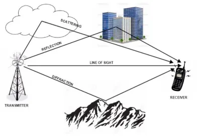
1.2.1 Multipath Fading
The electromagnetic waves used for transmission in wireless communication channels are broadcast through the communications medium. This implies that it is spread in multiple directions and encounters the effects of reflection from large buildings, diffraction from objects with sharp corners and scattering from the atmosphere, illustrated in figure 1.5 below. As a result, multiple copies of the transmitted signal with different strengths, delays and phase shifts arrive at the receiver and combine constructively and
7
Figure 1.5: Multipath Fading In Wireless Communication Channels
When the fading is such that the frequency components of the received signal undergo the same attenuation, this is known as Flat fading, as the channel has a relatively flat
frequency response over the signal bandwidth. However, when the fading is such that the frequency components of the signal undergo different attenuations, this is known as Frequency Selective fading. Flat fading and frequency selective fading can further be classified as slow fading, when the channel frequency response does not change within a frame length of data transmission and fast fading, when the channel response changes periodically within a frame length [34].
When the transmitter and receiver are separated by dense environments such as cities with tall buildings and structures, there is likely no direct link or Line of Sight (LOS) component of the transmitted signal at the receiver, but multipath components with varying attenuations and phase delays. The complex baseband representation of the received signal at the k th sampling time instant is:
8
where 𝑟(𝑘) ≡ 𝑟(𝑘𝑇𝑠), 𝑇𝑠 is the sampling period of the receiver, 𝜂(𝑘) is the sampled
Additive White Gaussian Noise (AWGN) at the receiver antenna, 𝑢(𝑘) is the complex baseband transmitted message and 𝛼(𝑘) = |𝛼(𝑘)|𝑒𝑗𝜃(𝑘) is a complex quantity
representing the fading between the transmitter and receiver. It has been shown in [34, 48] that, given this kind of environment with no LOS signal component at the receiver, the amplitude of the fading, |𝛼(𝑘)| can be modelled by a Rayleigh probability distribution and the phase shift, 𝜃(𝑘) can be modelled by a Uniform probability distribution between 0 and 2𝜋. Thus, this kind of channel is called a Rayleigh fading channel and the complex quantity 𝛼(𝑘) is called the Channel State Information (CSI) between the transmitter and receiver antennas. Rayleigh fading model is one of the most widely used for modelling wireless transmission [56] .
In this thesis, we consider a frequency-flat quasi-static (slow) Rayleigh fading channel model (implying that 𝛼(𝑘) = 𝛼 (𝑐𝑜𝑛𝑠𝑡𝑎𝑛𝑡) for the length of a data frame and changes from frame to frame) [23].
1.2.1.1
Diversity
In practice, in order to overcome the effects of fading on the received signals, different versions of the same signal are transmitted, such that each version undergoes independent fading. This technique is called Diversity. The expectation is that there is a greater chance of receiving a version that is not as severely faded as the others, improving the reliability of transmission. Thus, diversity takes advantage of the impairment imposed by fading. Diversity techniques popularly implemented include [27,28]:
Time Diversity: The same message signal is transmitted at multiple time periods.
Frequency Diversity: The same signal is transmitted at multiple frequencies.
Spatial Diversity: Diversity is achieved across space by transmitting the same signal from multiple antennas or receiving the same signal with multiple receiver antennas or a combination of both transmission techniques.
9
Among these diversity techniques, spatial diversity is one of the most widely used
techniques [1]. This is because of its ability to provide diversity gain (implying improved reliability of information transfer) and multiplexing gain (implying increased data rates), without consuming extra transmission bandwidth [23].It is broadly classified into diversity applied in single-user multiple-antenna communication (Multi-antenna
diversity) and diversity for multiple-user communication networks (Multiuser diversity) [1]. In this thesis, we focus on multi-antenna diversity.
The earliest form of multi-antenna diversity is the Single-Input Multiple-Output (SIMO) diversity, which implies the use of a single antenna at transmitter and multiple antennas at the receiver [14]. Diversity gain is achieved by combining the different received signals with methods such as Maximal Ratio Combining, and so on [19, 34]. This receive diversity is usually implemented at base station receivers.
Due to power and size limitations of mobile devices, receive diversity is not convenient for mobile receivers. However, a different form of multi-antenna diversity is the Multiple-Input Single-Output (MISO) diversity, which implies the use of multiple transmitter antennas and a single receive antenna. Works such as [22] show that this transmit
diversity enables designers to achieve diversity gain, while placing the burden of diversity on the base station transmitter, and achieving simple decoding complexity at the mobile receiver. This is achieved through the use of Space-Time Coding techniques, which are further explained in chapter 3.
Maximum diversity gain is achieved by using a spatial diversity technique called
Multiple-Input Multiple-Output (MIMO) diversity [45], implying a combination of both multiple transmitter and receiver antennas. This is also achieved by using space-time coding techniques at the transmitter.
10
Figure 1.6: Spatial Diversity Techniques
1.2.2
Carrier Frequency Offset
The process of demodulation explained in section 1.1 requires the receiver oscillator to produce a demodulating signal which has the same frequency as the carrier signal used for transmission. In other words, it is required that the transmitter and receiver oscillators are synchronized in frequency. However, in a practical scenario, there may be relative motion between the transmitter and the receiver, such as a mobile unit in a vehicle moving toward or away from the base station. This causes the signal which arrives at the receiver to experience a change in frequency at which it was transmitted. This behaviour
Tx Rx
SIMO
Rx MISO
Tx
Tx Rx
11
is called a Doppler shift. Also, due to device impairments, the transmitter and receiver oscillators may produce signals at different frequencies.
The frequency difference between the carrier signal and the receiver oscillator signal is called Carrier Frequency Offset (CFO). Let the frequency of the receiver oscillator signal be 𝑓𝑟 . The demodulation in (1.4) and (1.5) becomes:
Upper branch:
𝑟(𝑡) cos(2𝜋𝑓𝑟𝑡) = 𝑟𝐼cos(2𝜋𝑓𝑐𝑡). cos(2𝜋𝑓𝑟𝑡) − 𝑟𝑄sin(2𝜋𝑓𝑐𝑡). cos(2𝜋𝑓𝑟𝑡)
=𝑟𝐼
2{cos(2𝜋∆𝑓𝑡) [1 + cos(4𝜋𝑓𝑟𝑡)] − sin(2𝜋∆𝑓𝑡) sin(4𝜋𝑓𝑟𝑡)}
−𝑟𝑄
2 {sin(4𝜋𝑓𝑟𝑡) cos(2𝜋∆𝑓𝑡) + sin(2𝜋∆𝑓𝑡) . [1 + cos(4𝜋𝑓𝑟𝑡)]}
(1.7)
Lower branch:
𝑟(𝑡) sin(2𝜋𝑓𝑟𝑡) = 𝑟𝐼cos(2𝜋𝑓𝑐𝑡). sin(2𝜋𝑓𝑟𝑡) − 𝑟𝑄sin(2𝜋𝑓𝑐𝑡). sin(2𝜋𝑓𝑟𝑡)
=𝑟𝐼
2{sin(4𝜋𝑓𝑟𝑡) cos(2𝜋∆𝑓𝑡) − sin(2𝜋∆𝑓𝑡) . [1 − cos(4𝜋𝑓𝑟𝑡)]}
−𝑟𝑄
2{cos(2𝜋∆𝑓𝑡) [1 − cos(4𝜋𝑓𝑟𝑡)] + sin(2𝜋∆𝑓𝑡) . sin(4𝜋𝑓𝑟𝑡)}
(1.8)
where the CFO= ∆𝑓 = 𝑓𝑐− 𝑓𝑟
Low pass filtering the output of the demodulator branches yields 𝑟2𝐼cos(2𝜋∆𝑓𝑡) −
𝑟𝑄
2 sin(2𝜋∆𝑓𝑡) and
𝑟𝐼
2 sin(2𝜋∆𝑓𝑡)) +
𝑟𝑄
2 cos(2𝜋∆𝑓𝑡) in the upper and lower branches
respectively, which show the effect of CFO in degrading the quality of the received signal.
12
performance. Also, as communications standards move towards the direction of higher transmission frequencies with limited accuracy of receiver oscillators, the amount of CFO in these systems has become significant enough to pose problems[61].
1.3
Motivation of the Thesis
In order to overcome the effects of CSI and CFO on space-time coded communication systems, these parameters which are unknown to the receiver, have to be estimated and received signals have to be compensated for their presence. There has been numerous works published on the estimation of CSI and CFO, but these do not take into
consideration, the presence of estimation errors and the effects they have on signal detection.
Also, simplifying assumptions of these parameters and how they affect the received signals are usually made, in order to design estimation and detection schemes. However, these schemes may not be suitable for practical space-time coded communication
systems.
With the availability of practical models for estimation and detection in space-time coded systems faced with the problem of CSI and CFO estimation errors, it will be beneficial to study and provide insight into factors that are crucial for the desired system performance.
1.4
Objectives
Motivated by the issues discussed in section 1.3, the objectives of this thesis are outlined below:
Consider a practical model of the received signal in a space-time coded
13
optimal detection algorithm which considers the presence of CSI and CFO estimation errors.
Obtain estimator based on the described received signal model and implement the developed detection algorithm using this estimator, in order to examine its
performance.
Outline limitations on the estimator performance and compare their effects on conventional and proposed detectors.
1.5
Organization of the Thesis
The rest of the thesis is organized as follows. Chapter 2 gives a review of works
illustrating the development of space-time coding detection techniques and the attempts that have been made to overcome its challenges, after which we highlight the approach we intend to take to deal with these issues. Chapter 3 gives a review of space-time coding with emphasis on space time block coding (STBC) communication systems. The basic structure is illustrated with the popular Alamouti STBC scheme. The Maximum Likelihood (ML) detection scheme for Alamouti STBC receivers is described and we show the effects of imperfect CSI estimation and the presence of CFO on the performance of this receiver mathematically, and through performance simulations for different
modulation schemes.
In Chapter 4, we propose new ML detection algorithms in the presence of CSI and CFO estimation errors. We outline important assumptions and mathematical derivations for the proposed algorithms. Simulation results of the performance of these proposed detection algorithms against that of conventional ML detection algorithms are given at the end to show performance improvements over conventional detection.
14
Maximum Likelihood detection schemes when using these estimators, and we illustrate these with simulation results.
15
Chapter 2
Literature Review
In chapter 1, fading was discussed as a significant factor that affects wireless
communication systems and multi-antenna diversity was mentioned as the prominent means of combating fading effects. Early works on multi-antenna diversity techniques were published in the 1980s by Winters [15] and Salz [33]. However the works of Telatar [21] and Foschini [51] demonstrated that, from an information-theoretic perspective, significant improvements in capacity could be achieved using multi-antenna diversity instead of single-transmit single-receive antenna transmission and this led to a major push for the development of multi-antenna diversity techniques that can achieve these
improvements.[1] Multi-antenna diversity techniques are being applied in wireless communications standards such as Wireless Local Area Network (WLAN or IEEE 802.11n) standards [12], Fourth Generation(4G) mobile WiMAX and Long Term Evolution (LTE) standards. [17,35]
Multi-antenna diversity achieves the benefits of improved bandwidth and power efficiency in a fading environment through the application of space-time codes for transmission.[23] Tarokh et al. [22] proposed Space-Time Trellis Codes (STTC) for multi-antenna transmission. It uses a trellis coding structure [18] to arrange the
information to be transmitted across the multiple transmit antennas. STTCs enable the multi-antenna transmission schemes to attain both coding and diversity gain, but at the expense of increased decoder complexity. Alamouti [57] subsequently proposed the simplest form of Space-Time Block Codes (STBC) for two-transmit antenna
transmission. The orthogonal structure of the code allows for a reduction in decoder complexity, compared to STTC decoding, and full-rate transmission. STBCs were
16
Space-time codes have been used in conjunction with different receiver structures such as Maximum-Likelihood [57], Minimum Mean Square Error (MMSE), Zero-Forcing (ZF) and Vertical-BLAST (V-BLAST) receivers.[10] These receivers require Channel State Information to perform detection. Since perfect information is not available at the receiver, channel estimation is performed and the estimates are used instead. However, CSI estimates are imperfect and since these receivers are designed with the assumption that the CSI is perfectly known, the estimation errors will affect detection. Various works have been published on the effects of CSI estimation errors on space-time coding
detection schemes; effects such as the occurrence of error floors at high SNR regions, loss of coding gain, among others. [47, 50, 13]
Despite the presence of CSI estimation errors, efforts have been made to design detection schemes that can alleviate the effects of these errors. Tarokh [23] proposed a maximum likelihood detection scheme that incorporated statistical knowledge of the channel estimation error in the decision metric and demonstrated improvement in performance over detection using estimates only. Although he designed this for STTC transmission schemes, it can be generalized for other space time coding schemes. The work in [25] highlighted some incorrect assumptions made in [23] in designing the decision metric and proposed a detection scheme based on the correct assumptions of the statistical
relationship between fading channels. The work in [41] proposed a computationally efficient detection scheme that also incorporates statistical information about channel estimation error in the decision metric.
The works that have been discussed so far have assumed that there is perfect carrier frequency synchronization at the demodulator of the receiver, prior to detection.
17
However, these methods implicitly assume that the receiver has perfect knowledge of the channel, ignoring the need for channel estimation. Joint estimation of the CSI and CFO is therefore a more practical approach. This could be done by transmitting training symbols known to the receiver, or by blind estimation, relying only on the data symbols for information about CSI and CFO, as illustrated in [30, 55].
Though the works previously mentioned provide solutions for estimating the CSI and CFO, these works consider the CSI and CFO as deterministic (constant) but unknown. However, it is more practical to model them as random processes. Therefore, the previous works do not provide statistically optimal solutions to the CSI and CFO estimation
problem.
18
Chapter 3
Space-Time Coding
3.1 Introduction
In chapter 1, we saw that diversity is the method used to combat fading in wireless communications. Spatial diversity was highlighted as an important means of combating fading because of the benefits of improved reliability and increased data rates that it offers. It was also explained that spatial diversity can be achieved by using multiple antennas either at the transmitter or the receiver. However, considering the power and size restrictions imposed on mobile receivers, it is important to look for a feasible
alternative. The use of multiple transmitter antennas provides a feasible alternative, since base stations can accommodate more hardware to alleviate the size restrictions on mobile devices. Applying transmit diversity allows designers to achieve increased capacity, close to theoretical limits, reduced decoder complexity at the receiver and coding gain. These benefits are made possible through the use of multi-antenna coding schemes called Space-Time Codes. [22]
Space-time coding is the ordering of transmission information across multiple transmitter antennas (spatial domain) and multiple transmission periods (temporal domain) in such a way as to take advantage of the fading between the multiple transmit-receive links to achieve performance gains at the receiver. [16] Two important types of space-time codes are Space-Time Trellis Codes (STTC) and Space-Time Block Codes (STBC).
19
The simplest form of STBC was proposed by Alamouti [57] and is implemented with two transmitter antennas. Its orthogonal structure allows it to achieve full coding rate and diversity and significant reduction in the decoding complexity at the receiver. These features have promoted its application in wireless standards such as WCDMA [58] and CDMA2000 [60]. In this thesis, we apply the Alamouti STBC for frequency-flat fading channels and single receiver antenna.
This chapter gives a description of the Alamouti STBC transmitter and receiver structure. We then describe this transmission scheme in the presence of imperfect CSI, after which we consider the impact of imperfect frequency synchronization on STBC transmission and display performance results for these non-ideal scenarios.
3.2 STBC System Description
The Alamouti STBC communication system consists of:
a transmitter with an STBC encoder and two antennas for transmission
a receiver employing a Maximal-Ratio Combiner (MRC) and Maximum Likelihood decoder for detection.
3.2.1 STBC Transmitter
Figure 3.1below illustrates the process of STBC transmission. The information bits are mapped to 𝑁 symbols of a particular signal constellation. As illustrated by figure 3.1, for the case of an M-PSK or M-QAM signal constellation, 𝑁𝑏 bits are mapped to 𝑁 PSK or QAM symbols. These 𝑁 symbols are encoded into an 𝑁𝑡× 𝐿 STBC matrix:
𝑪 = [
𝑐1(1) 𝑐1(2) ⋯ 𝑐1(𝐿)
𝑐2(1) 𝑐2(2) ⋯ 𝑐2(𝐿)
⋮ ⋮ ⋱ ⋮
𝑐 𝑁𝑡(1) 𝑐 𝑁𝑡(2) ⋯ 𝑐 𝑁𝑡(𝐿)]
20
Figure 3.1: Space-Time Block Coding using 4-PSK modulation
where 𝑁𝑡 is the number of transmitter antennas and 𝐿 is the number of time periods for a STBC transmission. The ith row represents the symbols transmitted from the ith antenna and the jth column represents the symbols simultaneously transmitted from all antennas at the jth transmission period.
The Alamouti STBC takes N=2 symbols 𝑐1 and 𝑐2 and encodes them into the matrix:
𝑪 = [𝑐𝑐1 −𝑐2∗
2 𝑐1∗ ] (3.2)
which indicates that the Alamouti STBC transmitter transmits two symbols (N=2) simultaneously from two transmitter antennas over two transmission time periods (L=2). The rate of an STBC is defined as 𝑅 = 𝑁𝐿 therefore, the Alamouti STBC is a full-rate (R=1) code.
The rows of the Alamouti STBC are orthogonal to each other and this feature reduces the decoding complexity at the receiver.
The transmission symbols for each transmission time period modulate a high frequency sinusoidal carrier and are transmitted over a frequency-flat quasi-static Rayleigh fading channel. For the case of an Alamouti STBC communication system employing a single receiver antenna, the CSI between transmitter antenna 1 and the receiver antenna is 𝛼1(𝑡)
10 01 00 11
Symbol
Mapper
(b=2)
Spa
ce
-Ti
me
Enc
ode
r
𝑐
1(1)
…
𝑐
1(𝐿)
𝑐
2(1)
…
𝑐
2(𝐿)
𝑐
𝑁𝑡(1)
…
𝑐
𝑁𝑡(𝐿)
⁞
⁞
𝑥
1…
𝑥
𝑁1001010…
21
and the CSI between transmitter antenna 2 and the receiver antenna is 𝛼2(𝑡). The
quasi-static fading assumption implies that:
𝛼1(𝑡 + 𝑇𝑠) = 𝛼1(𝑡 + 2𝑇𝑠) = 𝛼1
𝛼2(𝑡 + 𝑇𝑠) = 𝛼2(𝑡 + 2𝑇𝑠) = 𝛼2 (3.3)
for 𝐿 = 2 and changes for different STBC transmissions. (𝑇𝑠 is the duration of a
transmission period.) In other words, the channel between the transmitter antennas and the receiver antenna remain fixed for the full frame length of STBC transmission and it differs for a different STBC transmission frame.
3.2.2 STBC Receiver
Figure 3.2: Space Time Block Coding Receiver
Figure 3.2 aboveis a block diagram of Alamouti STBC receiver with a single receiver antenna. Thisillustrates the complex baseband representation of reception and processing of STBC transmitted symbols. The received signals for both Alamouti STBC
transmission periods are given by:
Combiner Max im um L ikelihood De tec tor S y mbol De mappe r CSI Estimator
𝛼 1 𝛼 2
𝛼 1 𝛼 2
𝑐̂1
𝑐̂2
𝑐 1 𝑐 2
Data bits {𝜂(1), 𝜂(2)}
22
𝑟(𝑡 + 𝑇𝑠) = √𝐸𝑠(𝛼1𝑐1(𝑡 + 𝑇𝑠) + 𝛼2𝑐2(𝑡 + 𝑇𝑠)) + 𝜂(𝑡 + 𝑇𝑠)
𝑟(𝑡 + 2𝑇𝑠) = √𝐸𝑠(𝛼1𝑐1(𝑡 + 2𝑇𝑠) + 𝛼2𝑐2(𝑡 + 2𝑇𝑠))
+ 𝜂(𝑡 + 2𝑇𝑠)
(3.4)
For the sake of simplifying the notations used above, we write these received signals as: 𝑟(1) = √𝐸𝑠(𝛼1𝑐1(1) + 𝛼2𝑐2(1)) + 𝜂(1)
𝑟(2) = √𝐸𝑠(𝛼1𝑐1(2) + 𝛼2𝑐2(2)) + 𝜂(2) (3.5)
where 𝑟(1) and 𝑟(2) represent the complex baseband received signals obtained during the first and second STBC transmission period; 𝐸𝑠 is the average power of each
transmitted symbol; 𝜂(1) and 𝜂(2) represent the complex baseband Additive White Gaussian Noise (AWGN) at the receiver antenna for both STBC transmission periods and they can be modelled as complex Gaussian random processes ℂ𝒩(0, 𝑁0) with zero mean
and variance 𝑁0.
For Alamouti STBC transmission, the received signals can be written as: 𝑟(1) = √𝐸𝑠(𝛼1𝑐1+ 𝛼2𝑐2) + 𝜂(1)
𝑟(2) = √𝐸𝑠(−𝛼1𝑐2∗+ 𝛼2𝑐1∗) + 𝜂(2) (3.6)
or in matrix form as:
𝒓 = √𝐸𝑠𝑪𝑇𝜶 + 𝜼
[𝑟(1)𝑟(2)] = √𝐸𝑠[
𝑐1 𝑐2
−𝑐2∗ 𝑐 1∗] [
𝛼1
𝛼2] + [𝜂(1)𝜂(2)]
(3.7)
As shown in figure 3.2the receiver has a channel estimator which is assumed to give perfect CSI estimates. The combiner uses these CSI estimates together with the received signals to obtain the following symbols [57]:
𝑐 1 = √𝐸𝑠{𝛼1∗𝑟(1) + 𝛼2(𝑟(2))∗}
𝑐 2 = √𝐸𝑠{𝛼2∗𝑟(1) − 𝛼1(𝑟(2))∗}
23
3.2.2.1 Maximum Likelihood Detector
Maximum likelihood (ML) detection is a preferred form of signal detection in multi-antenna communication systems, as indicated in works such as [8, 29, 37, 46], which reveal that it yields satisfactory Bit Error Rate (BER) performance over other detection schemes.
The ML detection problem is to determine the pair of unknown parameters belonging to a discrete set of possible parameter pairs, given that we have a pair of observations with some information about the unknown parameters. We make this decision by maximizing a probability density function (pdf) called the Likelihood Function.
The detection problem can be described as a problem of maximizing the posterior pdf of the parameter pairs conditioned on the observations. In the Alamouti STBC detection problem, the unknown parameter pairs are the symbols transmitted, 𝒄 = [𝑐1 𝑐2]𝑇 while
the observations are the received signals and CSI estimates, [𝒓, 𝜶̂] where 𝒓 = [𝑟(1) 𝑟(2)]𝑇 and 𝜶̂ = [𝛼
1 𝛼 2]𝑇. Therefore, the detection problem can be described as:
𝒄 = arg max
𝒄∈𝝌 𝑃(𝒄|𝒓, 𝜶̂) (3.9)
where 𝝌is the discrete set of possible transmitted symbol pairs that can be obtained from the known modulation scheme employed at the transmitter. By Bayes theorem [36], this can be rewritten as:
𝒄 = arg max
𝒄∈𝝌
𝑃(𝒄). 𝑃(𝒓|𝒄, 𝜶̂)
𝑃(𝒓|𝜶̂) (3.10)
It is usually assumed that the symbols of the modulation scheme are equiprobable (they belong to a probability distribution with equal probabilities) [40]. Therefore, 𝑃(𝒄) is fixed and since the pdf 𝑃(𝒓|𝜶̂) is independent of 𝒄, the maximization problem simplifies to:
𝒄 = arg max
24
where 𝑃(𝒓|𝒄, 𝜶̂) is the likelihood function. Assuming that the CSI has been perfectly estimated (𝜶̂ = 𝜶), the likelihood function is conditionally Gaussian. Taking negative logarithm of the likelihood function reduces the maximization problem to:
𝒄 = arg min
𝒄∈𝝌 ‖𝒓 − √𝐸𝑠𝑪
𝑇𝜶‖ 𝐹
2 (3.12)
where ‖𝑨‖𝐹 is the Frobenius norm of 𝑨; 𝑪is given by (3.2)
Therefore, using Alamouti STBC, the maximum likelihood detector chooses the pair of symbols [𝑐̂1 𝑐̂2]𝑇 such that:
𝒄 = arg min
𝒄∈𝝌 {|𝑟(1) − √𝐸𝑠(𝛼1𝑐1+ 𝛼2𝑐2)| 2
+ |𝑟(2) − √𝐸𝑠(−𝛼1𝑐2∗+ 𝛼2𝑐1∗)| 2
} (3.13)
Using the symbols in (3.8) which were obtained from the combiner, the minimization problem can be rewritten as [57]:
𝒄 = arg min
𝒄∈𝝌 {𝐸𝑠(|𝛼1| 2+ |𝛼
2|2− 1)(|𝑐1|2+ |𝑐2|2) + 𝑑2(𝑐 1, 𝑐1) + 𝑑2(𝑐 2, 𝑐2)} (3.14)
where 𝑑2(𝑥, 𝑦) = |𝑥 − 𝑦|2 is the squared Euclidean distance between 𝑥 and 𝑦. The combiner symbols 𝑐 1, 𝑐 2 in (3.8) can be expanded as:
𝑐 1 = 𝐸𝑠(𝛼12+ 𝛼22)𝑐1+ √𝐸𝑠{𝛼1∗𝜂(1) + 𝛼2(𝜂(2))∗}
𝑐 2 = 𝐸𝑠(𝛼12+ 𝛼22)𝑐2− √𝐸𝑠{𝛼1(𝜂(2)) ∗
+ 𝛼2∗𝜂(1) } (3.15)
The equations in (3.15) show that, since the combiner symbols 𝑐 1, 𝑐 2 are functions of only 𝑐1 and 𝑐2 respectively, the ML detection in (3.14) can be split into two separate detection
schemes for 𝑐1 and 𝑐2 as:
𝑐̂1 = arg min
𝑐1∈𝝌
{𝐸𝑠(|𝛼1|2+ |𝛼2|2− 1)|𝑐1|2+ 𝑑2(𝑐 1, 𝑐1)}
𝑐̂2 = arg min
𝑐2∈𝝌
25
For equal energy constellations such as M-PSK, |𝑐1|2 = |𝑐2|2 = 1 for all possible values of 𝑐1 and 𝑐2 . Thus, 𝐸𝑠(|𝛼1|2+ |𝛼2|2− 1)|𝑐𝑖|2 is fixed and the detection can be further
simplified as:
𝑐̂1 = arg min
𝑐1∈𝝌
𝑑2(𝑐 1, 𝑐1)
𝑐̂2 = arg min
𝑐2∈𝝌
𝑑2(𝑐
2, 𝑐2) (3.17)
The simplified decoding complexity reflected in (3.16) and (3.17) is made possible by the orthogonal structure of the Alamouti STBC.
3.3 STBC Detection with Imperfect Channel
Estimation
The STBC detection process that was described in the previous section assumes that the channel state information is perfectly estimated at the receiver and the process relies on this assumption for optimum performance. However, the process of channel estimation involves the transmission of pilot symbols and their extraction from received signals at the receiver, in order to construct estimates of the channel fading between transmitter and receiver. Consequently, there are different factors which can degrade the performance of the estimator, such as the length of the pilot sequence transmitted, the power of
transmission; these lead to erroneous estimates at the receiver, which affect the performance of STBC detectors.
We illustrate the process of channel estimation using the Orthogonal Pilot Sequence Insertion method (OPSI) described in [23]. At the beginning of each data frame, we insert a sequence of pilot symbols 𝒄𝑝,𝑖, of sequence length 𝑙 at each transmitter antenna 𝑖:
𝒄𝑝,𝑖 = [𝑐𝑝,𝑖(1) 𝑐𝑝,𝑖(2) ⋯ 𝑐𝑝,𝑖(𝑙)] (3.18)
26
𝒄𝑝,𝑥 . 𝒄𝑝,𝑦𝐻 = 0 (3.19)
Let 𝒓𝑝,𝑚= [𝑟𝑝,𝑚(1) 𝑟𝑝,𝑚(2) ⋯ 𝑟𝑝,𝑚(𝑙)] be the sequence of received signals observed at the 𝑚th receiver antenna during the length 𝑙 training period. Therefore,
𝑟𝑝,𝑚(𝑘) = [∑ 𝑐𝑝,𝑢(𝑘). 𝛼𝑢,𝑚
𝑁𝑡
𝑢=1
] + 𝜂𝑝,𝑚(𝑘) (3.20)
where 𝑁𝑡 is the number of transmitter antennas, 𝛼𝑢,𝑚 is the CSI between the 𝑢th
transmitter antenna and the 𝑚th receiver antenna and 𝜼𝑝,𝑚 = [𝜂𝑝,𝑚(1) … 𝜂𝑝,𝑚(𝑙)] is the sequence of AWGN process at the receiver antenna 𝑚. The Minimum Mean Square Error (MMSE) estimate of the CSI 𝛼𝑢,𝑚 is given by [23]:
𝛼 𝑢,𝑚 =
𝒓𝑝,𝑚 . 𝒄𝑝,𝑢𝐻
𝒄𝑝,𝑢 . 𝒄𝑝,𝑢𝐻 (3.21)
Using (3.19) and (3.20), the CSI estimate can be expressed as:
𝛼 𝑢,𝑚 = 𝛼𝑢,𝑚+
𝜼𝑝,𝑚 . 𝒄𝑝,𝑢𝐻
𝒄𝑝,𝑢 . 𝒄𝑝,𝑢𝐻 (3.22)
From (3.22), we see that the CSI estimate consists of the actual CSI and an error term which will ultimately degrade the performance of the STBC detector. In general, the CSI estimate can be written as:
𝛼 𝑢,𝑚 = 𝛼𝑢,𝑚+ 𝛼𝑢,𝑚,𝑒 (3.23)
where 𝛼𝑢,𝑚,𝑒 is an error term. From (3.22), notice that the CSI is a complex Gaussian random process and the error term is a function of a complex Gaussian random noise process. Thus, the CSI estimate is also a random process.
27
3.3.1 Simulation of STBC Detector with
Imperfect Channel Estimation
In the previous section, we explained that channel estimation at the receiver is imperfect and this will in turn have negative consequences on the detector performance. We will now illustrate this by simulating an STBC communication system applying Alamouti STBC at the transmitter.
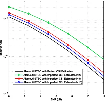
The simulated STBC communication system employs two transmitter antennas and one receiver antenna. The channels between each transmitter antenna and the receiver antenna are modelled as a complex Gaussian random process with zero mean and unit variance. The channel estimation at the receiver is performed using the MMSE estimator described in [23]. For each data frame transmitted, an orthogonal pilot sequence of length 𝑙 is transmitted at the beginning of the frame for channel estimation at the receiver. The variance of the estimation error for equal energy constellations (M-PSK) was given in [23]as:
𝜎𝑒𝑟𝑟𝑜𝑟2 = 𝑁0
𝑙𝐸𝑠
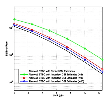
where 𝐸𝑠 is the energy of transmitted symbols and 𝑁0 is the variance of the noise process at the receiver. We simulate the transmission of 104 data frames for different Signal to Noise Ratio (SNR) values and evaluate the Bit Error Rate (BER) for each SNR value. The simulations were done for pilot sequence length 𝑙= 2,8,16, to illustrate the BER
28
Figure 3.3: Performance of 4-PSK STBC detector with imperfect CSI estimates Figure 3.3 shows the BER performance of an Alamouti STBC detector having imperfect CSI estimates when 4-PSK modulation is used for signal transmission. This illustrates the detector performance for signals transmitted from equal energy constellations. It can be observed that, for a fixed SNR, the detector BER performance when compared with the perfect CSI estimation case worsens as the pilot sequence length is limited from 𝑙 = 16 to
29
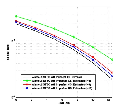
30
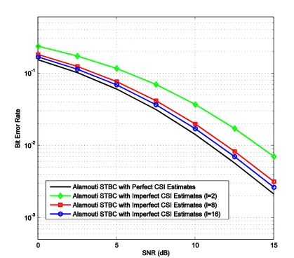
Figure 3.5: Performance of 16-PSK STBC detector with imperfect CSI estimates Figure 3.4 shows the BER performance of Alamouti STBC detector with 8-PSK
31
32
Figure 3.7: Performance of 16-QAM STBC detector with imperfect CSI estimates
Figures 3.6 and 3.7 illustrate the BER performance of an Alamouti STBC detector when the transmitted signals are selected from an unequal energy constellation (4-QAM and 16-QAM respectively). For a fixed BER, the SNR loss is much larger than the PSK
33
3.4 STBC Detection in the Presence of CFO
The STBC detection process that we have been discussing so far assumes that the receiver is perfectly synchronized in frequency with the transmitter. However, as discussed in section 1.2, in practice, this is not the case. The transmitted signal arrives at the receiver with a frequency which differs from that of the receiver oscillator. This difference in frequency is called Carrier Frequency Offset (CFO). For an Alamouti STBC receiver, the received baseband signal at the 𝑘th sampling instant after demodulation and filtering is obtained as:
𝑟(𝑘) = [∑ √𝐸𝑠𝑐𝑖(𝑘)𝛼𝑖𝑒𝑗2𝜋(∆𝑓𝑖)𝑘𝑇𝑠 2
𝑖=1
] + 𝜂(𝑘) ; 𝑘 = 1,2, … (3.24)
where ∆𝑓𝑖 = 𝑓𝑖 − 𝑓𝑟 is the CFO between the signal transmitted from antenna i and the receiver oscillator signal. (It is assumed that ∆𝑓𝑖 is fixed for an STBC transmission frame
and varies from frame to frame.) The received signal may be further represented as:
𝑟(𝑘) = [∑ √𝐸𝑠𝑐𝑖(𝑘)𝛼𝑖𝑒𝑗2𝜋𝜈𝑖𝑘 2
𝑖=1
] + 𝜂(𝑘) (3.25)
where 𝜈𝑖 is the CFO normalized by the sampling frequency. That is,
𝜈𝑖 = ∆𝑓𝑖𝑇𝑠 =
∆𝑓𝑖
𝑓𝑠 (3.26)
The normalized CFO 𝜈𝑖 can be decomposed into a fractional part and an integer part [62]
𝜈𝑖 = 𝜀𝑖 + 𝜆𝑖 (3.27)
where 𝜀𝑖 is the Fractional Frequency Offset (FFO) and 𝜆𝑖 is the Integer Frequency
Offset(IFO), which implies that 𝜆𝑖 is an integer and:
34
Inserting (3.27) into (3.25), we obtain:
𝑟(𝑘) = [∑ √𝐸𝑠𝑐𝑖(𝑘)𝛼𝑖𝑒𝑗2𝜋𝜀𝑖𝑘. 𝑒𝑗2𝜋𝜆𝑖𝑘 2
𝑖=1
] + 𝜂(𝑘) (3.28)
Since 𝜆𝑖 is an integer, the term 𝑒𝑗2𝜋𝜆𝑖𝑘 corresponds to a complete revolution and can be
neglected. Thus, the baseband received signal model reduces to:
𝑟(𝑘) = [∑ √𝐸𝑠𝑐𝑖(𝑘)𝛼𝑖𝑒𝑗2𝜋𝜀𝑖𝑘 2
𝑖=1
] + 𝜂(𝑘) (3.29)
Therefore, in this thesis, CFO refers to the fractional component of the normalized frequency offset in (3.29).
To illustrate the effect of CFO on STBC detection, consider the combining process in section 3.2, when there is no CFO present. An alternate way of representing the received signals at the Alamouti STBC receiver is:
[(𝑟(2))𝑟(1)∗] = √𝐸𝑠[
𝛼1 𝛼2
𝛼2∗ −𝛼
1∗] [
𝑐1
𝑐2] + [(𝜂(2))𝜂(1)∗] (3.30)
or in matrix notation, 𝒓 = √𝐸𝑠𝑯𝒄 + 𝜼.The combining process is given by 𝒄̃ = √𝐸𝑠𝑯𝐻𝒓 so that we obtain:
[𝑐 𝑐 1
2] = 𝐸𝑠[
|𝛼1|2+ |𝛼2|2 0
0 |𝛼1|2+ |𝛼2|2] [
𝑐1
𝑐2] + √𝐸𝑠[
𝛼1∗ 𝛼
2
𝛼2∗ −𝛼
1] [
𝜂(1)
(𝜂(2))∗] (3.31)
The equation (3.31) shows that, in the absence of CFO, the diagonal nature of 𝑯𝐻𝑯 allows the detection of symbols to be decoupled.
Now, considering the presence of CFO, the received signals may be represented as:
[(𝑟(2))𝑟(1)∗] = √𝐸𝑠[ 𝛼1𝑒
𝑗2𝜋𝜀1 𝛼2𝑒𝑗2𝜋𝜀2
𝛼2∗𝑒−𝑗2𝜋.2𝜀2 −𝛼1∗𝑒−𝑗2𝜋.2𝜀1] [
𝑐1
35
or in matrix notation, 𝒓 = √𝐸𝑠𝑯𝑒𝒄 + 𝜼. The equivalent combining process is given by 𝒄̃ = √𝐸𝑠𝑯𝑒𝐻𝒓so that we obtain:
[𝑐 𝑐 1
2] = 𝐸𝑠[
|𝛼1|2+ |𝛼
2|2 𝛼1∗𝛼2(𝑒𝑗2𝜋∆𝜀− 𝑒𝑗2𝜋.2∆𝜀)
𝛼2∗𝛼
1(𝑒−𝑗2𝜋∆𝜀− 𝑒−𝑗2𝜋.2∆𝜀) |𝛼1|2+ |𝛼2|2
] [𝑐𝑐1
2]
+√𝐸𝑠[𝛼1
∗𝑒−𝑗2𝜋𝜀1 𝛼2𝑒𝑗2𝜋.2𝜀2
𝛼2∗𝑒−𝑗2𝜋𝜀2 −𝛼1𝑒𝑗2𝜋.2𝜀1
] [(𝜂(2))𝜂(1)∗] (3.33)
where ∆𝜀 = 𝜀2− 𝜀1
Therefore, from (3.33), we observe that, in the presence of CFO, 𝑐 1 = 𝐸𝑠(|𝛼1|2+ |𝛼
2|2)𝑐1+ 𝐸𝑠[𝛼1∗𝛼2(𝑒𝑗2𝜋∆𝜀− 𝑒𝑗2𝜋.2∆𝜀)]𝑐2+ 𝜂𝑒,1
𝑐 2 = 𝐸𝑠(|𝛼1|2+ |𝛼
2|2)𝑐2+ 𝐸𝑠[𝛼2∗𝛼1(𝑒−𝑗2𝜋∆𝜀− 𝑒−𝑗2𝜋.2∆𝜀)]𝑐1+ 𝜂𝑒,2 (3.34)
where 𝜂𝑒,𝑖 is the i th row of 𝑯𝑒𝐻𝜼in (3.33). This shows that the presence of CFO
introduces an unwanted 𝑐2 term in the estimation of 𝑐1 and vice-versa, in estimating 𝑐2. This is called Inter-Symbol Interference (ISI).
36
3.4.1 Simulation of STBC Detector in the
presence of CFO
This section illustrates the performance of an Alamouti STBC detector which uses a single receiver antenna, with CFO present in the system. This detector, which was described in section 3.2, assumes perfect estimation of the CSI and perfect
synchronization at the receiver. Therefore, in the simulation, it was assumed that the CSI is perfectly estimated at the receiver, to highlight the effects of CFO on signal
transmission.
The Rayleigh fading channel model, same as that in section 3.3.1 was used for the simulation and the received signal was modelled using (3.29). The CFO 𝜀𝑖 between the signal transmitted from antenna i and the receiver oscillator signal is modelled as a Uniform random process. That is,
𝜀𝑖 ∼ 𝑈𝑛𝑖𝑓𝑜𝑟𝑚 [−𝛽, 𝛽]; 𝛽 ∈ (0,0.5)
37
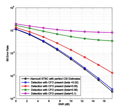
Figure 3.8: Performance of 4-PSK STBC detector with CFO present
38
39
40
41
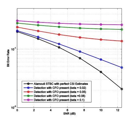
Figure 3.12: Performance of 16-QAM STBC detector with CFO present
Figures 3.11 and 3.12 show the performance of the detector when 4-QAM and 16-QAM modulation schemes are used for transmission. The results show that the performance degradation is more severe than for the case of PSK modulation. This implies that the presence of CFO would have a more devastating effect on unequal-energy modulation schemes compared to equal energy modulation schemes.
42
Chapter 4
Maximum Likelihood Detection Algorithms
In The Presence Of CSI and CFO Estimation
Errors
In this chapter, we discuss Maximum Likelihood detection algorithms for space-time coded communication systems, in the presence of CSI and CFO estimation errors. A model for the CSI and CFO estimates is stated and ML detection algorithms are derived, based on different assumptions for the CSI and CFO estimation errors. The performance plots for these communication systems modelled by these assumptions are also illustrated in this chapter.
4.1 Assumptions
Let us consider an Alamouti STBC communication system using two transmitter antennas and one receiver antenna. Works such as [40, 43]assume that all transmit antennas share a common CFO with the receiver antenna. However, Stoica [55]pointed out the fact that this is valid only when the multipath fading components are incident on the receiver antenna from a common angle of arrival, hence a general model includes multiple CFOs between the different transmit-receive antenna pairs. Therefore, the complex baseband received signal in the presence of fading and imperfect synchronization, at sampling time instant k, 𝑟(𝑘) is given by
𝑟(𝑘) = [√𝐸𝑠 ∑ 𝛼𝑖
2
𝑖=1
43
where 𝑐𝑖(𝑘) is the symbol transmitted from antenna i at time instant k, 𝐸𝑠 is the symbol
transmit power, 𝛼𝑖 is the CSI between transmitter antenna i and the receiver antenna, 𝜀𝑖 is the CFO between transmitter antenna i and the receiver antenna, and 𝜂(𝑘) is the baseband noise at the receiver antenna. The symbols 𝑐𝑖(𝑘) are assumed to be selected from a
constellation with unit average energy.
In this thesis, Rayleigh fading is considered. Therefore, the CSI is considered to be a complex Gaussian random process ℂ𝒩(0, 𝜎𝛼2) with zero mean and variance 𝜎𝛼2 .
As explained previously in chapter 3, 𝜀𝑖 represents the fractional part of the CFO which is solely responsible for imperfect frequency synchronization in the received signal model described above. Works such as [44, 53]emphasize the fact that, contrary to early works on frequency synchronization errors which modelled the CFO as deterministic variables, it is more practical to model CFOs as random processes, due to the random nature of variation of the accuracy of local oscillators. These works consider the CFO to be a zero mean Gaussian random process.
However, as highlighted in [9],it is more practical to consider the CFO to be limited in range. Therefore, contrary to the previous Gaussian assumption, this thesis considers CFO 𝜀𝑖 as Uniformly distributed random processes within the range[−𝛽, 𝛽] (That is,
𝜀𝑖~𝑈𝑛𝑖𝑓𝑜𝑟𝑚[−𝛽, 𝛽], 𝛽 ∈ (0,0.5) ) and independent of each other.
The baseband noise 𝜂(𝑘)is modelled as a complex Additive White Gaussian Noise (AWGN) process ℂ𝒩(0, 𝑁0) with zero mean and variance 𝑁0 .
44
4.2 Maximum Likelihood (ML) Detection
The ML metric given by Tarokh [23]is considered to be the standard metric for optimum detection in space-time coded systems with Rayleigh fading channels. The ML detection, after CSI estimation is performed is given by:
𝒄 = 𝑎𝑟𝑔 max
𝒄∈𝜒 𝑃(𝒓|𝒄,𝜶̂) (4.2)
where 𝒄 is the detected transmission symbol vector chosen from the set 𝜒 of possible transmitted symbols, which maximizes the above probability density function (pdf); 𝜶̂ is the vector of CSI estimates and 𝒓 is the complex baseband received signal vector.
Tarokh [23]showed that, assuming 𝑃(𝑟(𝑘)|𝒄,𝜶̂) is a conditionally Gaussian pdf, taking the negative logarithm of the likelihood function reduces the above maximization problem to:
𝒄 = 𝑎𝑟𝑔 min
𝒄∈𝜒 ∑ (𝐿𝑛(𝑉𝑎𝑟[𝑟(𝑘)|𝒄,𝜶̂]) +
|𝑟(𝑘) − 𝐸[𝑟(𝑘)|𝒄,𝜶̂]|2
𝑉𝑎𝑟[𝑟(𝑘)|𝒄,𝜶̂] )
2
𝑘=1 (4.3)
where 𝐸[𝑟(𝑘)|𝒄,𝜶̂] and 𝑉𝑎𝑟[𝑟(𝑘)|𝒄,𝜶̂] are to be determined.
For this thesis, assuming that the transmitted symbols are equiprobable, the ML detection after obtaining CSI and CFO estimates 𝜶̂, 𝜺 is given by:
𝒄 = 𝑎𝑟𝑔 max
𝒄∈𝜒 𝑃(𝒓|𝒄,𝜶̂, 𝜺 ) (4.4)
45
In the same line of argument, we assume that the pdf 𝑃(𝑟(𝑘)|𝒄,𝜶̂, 𝜺 ) is conditionally Gaussian. Thus, similar to Tarokh metric above, the ML detection, in the presence of CSI and CFO estimation errors, reduces to
𝒄 = 𝑎𝑟𝑔 min
𝒄∈𝜒 ∑ (𝐿𝑛(𝑉𝑎𝑟[𝑟(𝑘)|𝒄, 𝜶̂, 𝜺 ]) +
|𝑟(𝑘) − 𝐸[𝑟(𝑘)|𝒄, 𝜶̂, 𝜺 ]|2
𝑉𝑎𝑟[𝑟(𝑘)|𝒄, 𝜶̂, 𝜺 ] )
2
𝑘=1
(4.5) This can be generalized for an arbitrary number of receive antennas. The estimates of a parameter can be modelled as a sum of the actual parameter and an error term. Thus, the estimates 𝛼 𝑖 and𝜀̂𝑖 can be modelled as:
𝛼 𝑖 = 𝛼𝑖 + 𝛼𝑖,𝑒 (4.6)
𝜀̂𝑖 = 𝜀𝑖+ 𝜀𝑖,𝑒 (4.7)
where 𝛼𝑖,𝑒and 𝜀𝑖,𝑒 are the CSI and CFO estimation errors, respectively.
Next, we derive ML detection algorithms for different sets of assumptions for CSI and CFO estimation errors.
4.2.1 Case I:
𝜶
𝒊,𝒆
is Complex Gaussian and
𝜺
𝒊,𝒆
is Gaussian
In this case, CSI estimate 𝛼 𝑖 = 𝛼𝑖 + 𝛼𝑖,𝑒 , where 𝛼𝑖 is ℂ𝒩(0, 𝜎𝛼2) and 𝛼𝑖,𝑒 is ℂ𝒩(0, 𝜎𝛼2𝑒).