Spectrum Occupancy Estimation and Analysis

(1)

Electronic Theses and Dissertations Theses, Dissertations, and Major Papers

9-16-2019

Spectrum Occupancy Estimation and Analysis

Danilo Roberto Corral-De-Witt University of Windsor

Follow this and additional works at: https://scholar.uwindsor.ca/etd

Recommended Citation Recommended Citation

Corral-De-Witt, Danilo Roberto, "Spectrum Occupancy Estimation and Analysis" (2019). Electronic Theses and Dissertations. 7803.

https://scholar.uwindsor.ca/etd/7803

This online database contains the full-text of PhD dissertations and Masters’ theses of University of Windsor students from 1954 forward. These documents are made available for personal study and research purposes only, in accordance with the Canadian Copyright Act and the Creative Commons license—CC BY-NC-ND (Attribution, Non-Commercial, No Derivative Works). Under this license, works must always be attributed to the copyright holder (original author), cannot be used for any commercial purposes, and may not be altered. Any other use would require the permission of the copyright holder. Students may inquire about withdrawing their dissertation and/or thesis from this database. For additional inquiries, please contact the repository administrator via email

(2)

and Analysis

by

Danilo Roberto C

ORRAL

D

E

W

ITT

A Dissertation

Submitted to the

Faculty of Graduate Studies

through

the Department of

Electrical and Computer Engineering

in Partial Fulfillment of the Requirements for

the Degree of

Doctor of Philosophy

at the University of Windsor

Windsor, Ontario, Canada

2019

c

(3)

and Analysis

by

Danilo Roberto C

ORRAL

D

E

W

ITT

APPROVED BY:

I. Mora-Jiménez, External Examiner

Universidad Rey Juan Carlos

Z. Kobti

School of Computer Science

E. Abdel-Raheem

Department of Electrical and Computer Engineering

B. Balasingam

Department of Electrical and Computer Engineering

K. Tepe, Advisor

Department of Electrical and Computer Engineering

(4)

Declaration of Co-authorship /

Previ-ous Publications

I. Co-authorship

I hereby declare that this thesis incorporates material that is a result of joint research. This thesis contains the outcome of research undertaken by me un-der the supervision of Dr. K. E. Tepe with the collaborative help from my col-leagues in WiCIP lab in the form of advice, critiques, observations, and men-toring. This thesis also reflects the outcomes of joint work realized with Aar-ron Younan, Arooj Fatima, Jose Matamoros-Vargas, Dr. Faroq Awin, Dr. Esam Abdel-Raheem, Dewan M. Ariful, Lining Zhang, Dr. Sabbir Ahmed, and Dr. Jose Luis Rojo-Álvarez. The mathematical analysis, probabilistic model, data collected, results obtained and presented among the thesis were the outcome of this joint research and collaboration. In all cases, the key ideas, primary con-tributions, experimental designs, data collection, analysis and interpretation, were performed by the author of this thesis, and the contribution of co-authors was primarily through the provision of valuable suggestions and help in the comprehensive analysis of the experimental results submitted for the published articles.

I am aware of the University of Windsor Senate Policy on Authorship and I certify that I have properly acknowledged the contribution of other researchers to my thesis, and have obtained written permission from each of the co-author(s) to include the above material(s) in my thesis.

I certify that, with the above qualification, this thesis, and the research to which it refers, is the product of my own work.

II. Previous Publications

(5)

Thesis Chapter

Publication title/full citation Publication

status

Part of Chapter 1, 2, and 3

Corral-De-Witt, D., Younan, A., Fatima, A., Mata-moros, J., Awin, F. A., Tepe, K., & Abdel-Raheem, E. (2017, April). Sensing TV Spectrum Using Soft-ware Defined Radio HardSoft-ware. In 2017 IEEE 30th Canadian Conference on Electrical and Computer Engineering (CCECE) (pp. 1-4). IEEE.

Published

Part of Chapter 3, 4 , and 5

Corral-De-Witt, D., Younan, A., Ariful, D., Zhang, L., & Tepe, K. (2018, August). Multiplatform Spec-trum Sensing Prototype. In 2018 IEEE 61st Inter-national Midwest Symposium on Circuits and Sys-tems (MWSCAS) (pp. 198-201). IEEE.

Published

Part of Chapter 2

Hassan, D. M. A.,Corral-De-Witt, D., Ahmed, S., & Tepe, K. (2018, December). Narrowband Data Transmission in TV White Space: An Experimental Performance Analysis. In 2018 IEEE International Symposium on Signal Processing and Information Technology (ISSPIT) (pp. 252-257). IEEE.

Published

Part of Chapter 4, 5, and 6

Corral-De-Witt, D., Ahmed, S., Awin, F., Rojo-Álvarez, J. L., & Tepe, K. (2019). An Accurate Prob-abilistic Model for TVWS Identification. MDPI Ap-plied Sciences.

Submitted

I certify that I have obtained a written permission from the copyright owner(s) to include the above published material(s) in my thesis, as observed in Ap-pendix A. I certify that the above material describes work completed during my registration as a graduate student at the University of Windsor.

III. General

(6)

a written permission from the copyright owner(s) to include such material(s) in my thesis.

(7)

Abstract

(8)

Dedication

(9)

Acknowledgements

I sincerely want to thank all the persons and institutions who were involved in the development of this research project:

To Dr. Kemal Tepe, who encouraged me to develop this research, and all the time was aware of my progress and results.

To Dr. Esam Abdel-Raheem, Dr. Balakumar Balansingam, and Dr. Ziad Kobti, the Ph.D. Committee Members, for all the advisory, recommendations and feedback received during these years.

To Dr. Inmaculada Mora Jiménez, External Committee Member for agreed to be part of this project.

To my professors, lecturers, authorities, technical team, and all the adminis-trative personnel of the University of Windsor, especially to Ms. Andria Ballo, for supporting me during the development of this research.

To SENESCYT and Universidad de las Fuerzas Armadas ESPE of Ecuador, for its support and the facilities provided in the development of my Ph.D. pro-gram.

(10)

List of Figures

2.1 CR cycle, the spectrum is sensed, analyzed, and a decision is taken based on the presence or absence of PUs. . . 8 2.2 Use of TVWS to provide communications to the First Response

Institutions (FRI) and the Public Safety Answering Point (PSAP) during an earthquake. . . 11 2.3 Diagram of the E-call procedure, the accident vehicle send a

mes-sage through the idle channels of TV spectrum to reach the near-est PSAP. . . 12

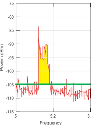
3.1 Graphical representation of Energy Detection when peaks of the signal contain a power (yellow area) higher than the Threshold (green line). . . 14 3.2 Overlapped plots for the composed signal in red and noise in

blue, (a) for RFE and (b) for SA. . . 15 3.3 Pilot tone detected in channel 20 (506.31MHz±100KHz). . . 16 3.4 Proposed SSS to sense spectrum in indoor and outdoor fixed

lo-cations. . . 18 3.5 A portable version of the SSS used to sense indoor spectrum. . . 20 3.6 Initial diagram for the M-SSS, designed to be mounted in a

vehi-cle and sense the TV spectrum in wide geographical areas. . . 21 3.7 M-SSS (a) design diagram, (b) station mounted, (c) supporting

structure built in CPVC, (d) supporting installed in the vehicle, (e) Winegard and GPS antennas, and (f) M-SSS in operation. . . . 22 3.8 TV Signal sensed an RFE (blue line) and a SA (red line) are

com-pared. The general shape that contains the energy is easily iden-tified in the plot obtained with both devices. . . 24 3.9 Trajectories and locations to represent the TV spectrum sensed in

the city of Windsor. . . 25 3.10 Visualization of the TV signal sensed using an RFE device, the

(14)

4.1 TV Signal sensed with (a) RFE and (b) SA are compared. The general shape that contains the energy under the red line is easily identified in both devices. . . 28 4.2 Proposed M-SSS to sense in parallel the NoiseW(f)and the

com-posite signalX(f). . . 29 4.3 TV Signal sensed with (a) RFE and (b) SA are compared. The

W(f)andX(f)are observed and permit infer their possible rela-tionship. . . 29 4.4 TV Signal sensed with (a) RFE and (b) SA are compared. The

W(f) and X(f)are observed and it is considered the noise level for that specific data collected. . . 30 4.5 Comparison of the signal sensed with (a) RFE and (b) SA. In both

sub-figures are plotted X(f), W(f), and the different values for

MorT. . . 31 4.6 Noise signal sensed W(p). (a) Histogram of the collected data.

(b) Normal probability plot of the same data read. (c) CDF of the Kolmogorov-Smirnov Test (KST) applied. . . 32 4.7 Composite signal plus noise sensed Xo(p). (a) Histogram of the

collected data. (b) Normal probability plot of the distribution for the same reading (c) CDF of the Kolmogorov-Smirnov Test (KST) applied. . . 33 4.8 The curve Xo(p) of the multi-modal distribution of (a) can be

assumed as the normal distribution curve X(p) of (b), this as-sumption summarized in (c) allow us to reduce the calculation complexity of the proposed model. . . 33 4.9 Readings taken in three different points, the pdf for the noise

W(p) is plotted in blue, multi-modal composite signalXo(p) in magenta, and composite signal X(p)in red. In (a) are shown the pdf of the noise for each location. In (b), the intersection point "A" of W(p)∩Xo(p) and its projection to the power axis "A0". In (c), the intersection point "B" ofW(p)∩X(p), and its projection to the power axis "B0", we also observe that the difference between

A0 and B0 is minimum concerning the power level of the signal in dBm. . . 34 4.10 Normal distribution pdfs forW(p) in blue and assumedX(p)in

red, both used to calculate the Pf a and the Pd according to the

(15)

4.11 Neyman Pearson model, the null hypothesis and the alternative hypothesis are observed. . . 36 4.12 Pdf ofW(p)in blue andX(p)in red, taken from the data collected

with (a) RFE and (b) SA. . . 37 4.13 Graphical representation of the Pm, Pf a, and Pd, generated by the

Tand the pdf curves forW(p)andX(p). . . 38 4.14 Minimum and maximum possible values forM. . . 39 4.15 pdf of theW(p) andX(p)taken from the data read with (a) RFE

and (b) SA, the Mminand Mmax are identified. . . 40

4.16 Comparison of the signal sensed with (a) RFE and (b) SA. In both panels the adaptiveTis plotted, comparing with the Tproposed by other related works. . . 42 4.17 Composite signal and noise sensed in point P11, (a) Frequency vs

power, (b) pdf of the sensed signals. . . 42 4.18 Visual representation of a Tthat observes aPf a=3%. . . 43

4.19 ROC: (a) for the proposed model with the area of interest coloured; (b) for Neyman Pearson model. . . 43 4.20 Detailed ROC curve for samples taken. . . 44

5.1 Proposed SSS for fixed outdoor and portable indoor sensing pur-poses. . . 46 5.2 Portable SSS to sense the spectrum in indoor environments. . . . 47 5.3 Attenuation introduced by the splitter, the theoretical value is 7

dB, (a) for RFE and (b) for SA. . . 47 5.4 Applications used to collect data, (a) for RFE, (b) for SA, and (c)

for RTL-SDR. . . 48 5.5 M-SSS to sense spectrum over a mobile platform to sense wide

geographical areas, (a) original diagram, (b) proposed configura-tion. . . 49 5.6 Data collection, 1 reading is composed by 112 samples for the

composite signal, 112 samples for noise, separation between two samples is 1.76 MHz, all 112 samples covers 198 MHz which is the UHF TV bandwidth. . . 51 5.7 Proposed SSS for fixed and portable sensing purposes in outdoor

and indoor environments. . . 52 5.8 Proposed M-SSS to sense spectrum over a mobile platform to

sense wide geographical areas. . . 53 5.9 Proposed M-SSS to sense spectrum over a mobile platform to

(16)

5.10 Proposed graphical representations of results. . . 55

6.1 Four trajectories were defined to sense the UHF TV spectrum in the city of Windsor, T1 red, T2 purple, T3 blue, and T4 orange. . . 57 6.2 P11 (a) Spectrum diagram, (b) pdf of the noise and composite

signal, and (c) Receiver Operation Characteristics curve with the

Pf a vsPd. . . 58

6.3 Sub-figures(a)to(j)spectrum vs power sensed in Points 1 - 10, there are variations on the energy detected due to the different location in which the samples were taken. . . 59 6.4 Sub-figures(a) to(j) pd f of theW(p)andX(p)sensed in Points

1 - 10. . . 60 6.5 Sub-figures(a)to(j)ROC curves of the signal sensed in Points 1

to 10. . . 61 6.6 ROC curves obtained from P1 - P10, in (a) are present all the

curves, and in (b) are shown the same plot but zooming in to observe the curves with a Pf a closer to the one defined by the

adaptive Tof 3%. . . 62 6.7 Dotted lines are the Pf amax, Pf a calculated with the adaptive T,

and T obtained by using a Mof 5, 7, and 10dBrespectively. It is observed that the adaptive T proposed increases at lest 9.63% of

Pdthan the values used by other authors. . . 63

6.8 Location of the represented points . . . 64 6.9 Spectrum detected and analyzed with the proposed model. (a)

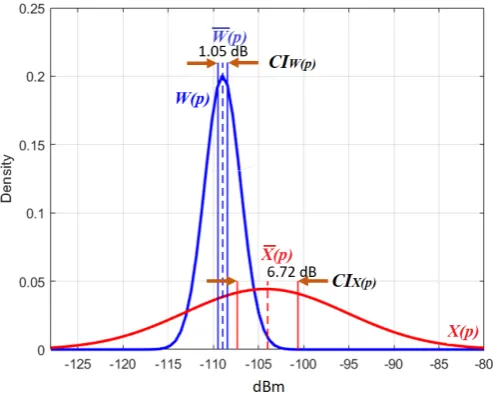
central south part of the city, (b) southeast, (c) middle east, and (d) eastern limit of the city of Windsor. Note that as far of the center the sample is taken, less PU are detected. . . 65 6.10 Plot of the Confidence Interval (CI) of average values for W(p)

(17)

List of Tables

2.1 Bands assigned to the TV broadcasting service, frequencies,

chan-nel numbers, partial Bandwidth (BW), and ITU regions. . . 5

2.2 UHF TV channels with their characteristics frequencies in MHz. . 7

3.1 Active TV channels received in Windsor area. . . 17

3.2 DAI’s features and performance comparison . . . 25

3.3 Trajectories defined to sense the TV spectrum in the city of Windsor 26 4.1 Estimated values forPf a, F(z), andz. . . 41

5.1 Communication from the three DAI to the PC to save data col-lected in the DB. . . 48

5.2 Communication from the three DAI to the PC to save data col-lected in the DB. . . 49

5.3 Distance between data readings and speed. . . 50

5.4 Decision Procedure, true table. . . 55

(18)

List of Abbreviations

AWGN Additive White Gaussian Noise

BS Base Station

CAD Canadian Dollar

CBD Co-variance Based Detection

CDF Cumulative Density Function

CEI Centre for Engineering and Innovation

CI Confidence Interval

CPVC Chlorinated Polyvinyl Chloride

CR Cognitive Radio

CSD Cyclo-Stationary Detection

CSV Comma Separated Values

DAI Data Acquisition Instrument

DB Database

dB Decibel

dBm Decibel with reference to one milliwatt

DSA Dynamic Spectrum Access

ED Energy Detection

EDRC Emergencies and Disaster Relief Communications

FCC Federal Communications Commission

FRI First Response Institutions

GHz Gigahertz

GPS Global Positioning System

HD High Definition

IEEE Institute of Electrical and Electronic Engineers

ISM Industrial, Scientific and Medical

IoT Internet of Things

ITU International Telecommunications Union

KHz Kilohertz

KST Kolmorogov-Smirnov Test

M Margin

Mmin Minimum Margin

(19)

MFD Matched Filtering Detection

MHz Megahertz

ML Machine Learning

M-SSS Mobile Spectrum Sensing Station

OS Operating System

PD Pilot Detection

Pd Probability of Detection

pdf Probability Density Function

Pfa Probability of False Alarm

PHY Physical Layer

Pm Probability of Missed-detection

PSAP Public Safety Answering Point

PU Primary User

RBW Resolution Bandwidth

RF Radio Frequency

RFE Radio Frequency Explorer

ROC Receiver Operating Characteristic

RTL-SDR Register-Transfer Level Software Defined Radio

SA Spectrum Analyzer

SD Standard Definition

SDR Software Defined Radio

SSS Spectrum Sensing Station

SU Secondary User

T Threshold

TDR Telecommunications for Disaster Relief

Tmax Threshold maximum

Tmin Threshold minimum

TVBS Television Black Spaces

TVGS Television Gray Spaces

TVWS Television White Spaces

UHF Ultra High Frequency

U-NII Unlicensed National Information Infrastructure

USB Universal Serial Bus

WiCIP Wireless Communications and Information Processing Lab

WLAN Wireless Local Area Network

WRAN Wireless Regional Area Network

WS White Spaces

(20)

Chapter 1

Introduction

In the last 10 years, the world has experienced impressive growth in wireless communication technologies leading to the emergence of new devices and ser-vices at an unprecedented pace. This, in turn, has created a great and ever-increasing demand for electromagnetic spectrum for data transfer. Usage of the electromagnetic spectrum, as it stands today, shows a peculiar characteristic. While some parts of the spectrum are extremely crowded, some other parts are underutilized. Thus there is scarcity as well as wastage [1], [2].

Cognitive Radio or CR that proposes smart sharing of the unused frequen-cies can be a promising solution to increasing spectrum usage efficiency. CR uses different spectrum sensing techniques to detect unused channels and then allows opportunistic usage of such channels by Secondary Users (SU), i.e., un-licensed users, without interfering with Primary Users (PU), i.e., un-licensed users. The unused electromagnetic spectrum bands are known as White Spaces (WS), and the technique of opportunistically using the WS is called Dynamic Spec-trum Access (DSA). Again, WS that fall in the electromagnetic specSpec-trum bands used by Television broadcasting services is known as TV White Spaces (TVWS) [3]. Irrespective of which spectrum is being used, CR requires that harmful in-terference to PU must be avoided at all time.

TV spectrum bands often show underutilization by PU and hence use of TVWS in CR is a promising solution to spectrum scarcity. In context to this, the Institute of Electrical and Electronics Engineers (IEEE) approved the 802.22 standard in 2011 [4]. But finding a model that allows accurate identification of TVWS, minimizing false alarms and errors is a challenging issue.

1.1 Research Objectives

(21)

Alarm (Pf a) and the Probability of Detection (Pd) of the sensed signals. Thus the

research objectives are:

• To develop a probabilistic and accurate model to identify TVWS.

• To design and implement a Spectrum Sensing Station (SSS) and a Mobile Spectrum Sensing Station (M-SSS).

• To find the best low-cost detector for TVWS.

• To collect, analyze, and find the characteristics of the data related to UHF TV Spectrum in the city of Windsor - ON, Canada.

1.2 Radio Electrical Spectrum Basics

Radio spectrum is a part of the electromagnetic spectrum that corresponds to the frequencies used by wireless based communications, i.e., radio, TV, cell-phone companies, satellite services, and more. The frequency used for each service has a direct relationship between distance and data rate that the signal can transmit [5].

There are two types of frequency bands, licensed and unlicensed. The first group requires a payment of a licensing fee to use it, which implies the exclusiv-ity and the certainty of no interference from other wireless users [6]. The local regulation authority is the entity that manages the radio-electrical spectrum and obtains funds from the auction of those licensed bands. The second group are the unlicensed bands, which do not require any permissions or payment for use the spectrum, but for that reason, they are vulnerable to interference due to the reduced number of unlicensed bands and the increasing number of users that are competing for accessing to those free bands.

(22)

To solve this scarcity, the use of CR has been proposed [7]. The Interna-tional Telecommunications Union (ITU) defines CR as “A radio system employ-ing technology that allows the system to obtain knowledge of its operational and ge-ographical environment established policies and its internal state; to dynamically and autonomously adjust its operational parameters and protocols according to its obtained knowledge in order to achieve predefined objectives, and to learn from the results ob-tained”[8].

1.3 Motivation

The motivation of this research endeavour is to use CR techniques to discover TVWS for other spectrum demanding wireless services and applications. For example, Wireless Regional Area Networks (WRAN), internet access for ru-ral areas, Wireless Sensor Networks (WSN), Emergency Communications (EC), and Telecommunications for Disaster Relief (TDR). Particularly, the last two ap-plications, i.e., EC and TDR, attracted all my attention because they are both related to rescuing lives. With a long experience in public safety issues, i.e., as a former member of the armed forces and as part of the 911 emergency services implementation team, I feel that using CR based wireless communications as the communications platform, should be given a priority for providing emer-gency services. For this, the first step is to identify which frequencies can be used to provide those services. Again for identifying available frequencies, a probabilistic model is needed, complemented with a novel low-cost sensing technique.

1.4 Contributions

The contributions in this thesis can be divided into four parts, e.g. technique and configuration of the sensing hardware used, sensing techniques applied, probabilistic model applied, and results of the sensed spectrum in the city of Windsor.

• Propose a technique that senses the spectrum in a different manner that considers the simultaneous use of hardware to measure the noise and the composite signal and noise, to improve detection accuracy.

(23)

• The develop a probabilistic model consisting of false alarm probability and detection probability to ensure better results than other methods ap-plied to identify TVWS.

• A prototype was designed and implemented to demonstrate the devel-oped technique for TVWS spectrum sensing. This prototype was used to sense the spectrum across the city of Windsor in Canada.

1.5 Thesis Organization

This dissertation is composed of 6 chapters.

Chapter 1 provides an introduction, contributions of the research, and ex-plains the general organization of the document.

Chapter 2 presents the background and motivation for the study. Major con-cepts used, a brief discussion of the applications of TVWS in telecommunica-tions, and a special mention in telecommunications for disaster relief.

Chapter 3 provides TVWS concepts, spectrum bands used, sensing tech-niques, and additional parameters needed to understand and exploit the smart spectrum sharing.

Chapter 4 presents the mathematical and statistical considerations oriented to identify the parameters that take part in this dissertation, characteristics of the sensed signals, probabilities, and more related information.

Chapter 5 presents the proposed model, the hardware configuration to sense the spectrum results obtained in the survey conducted along the city of Wind-sor, and the contributions.

Chapter 6 describes the results obtained in the survey and information col-lected in the city of Windsor.

(24)

Chapter 2

Background

In this chapter, the basic concepts of spectrum, TVWS, CR fundamentals, Litera-ture review, applications and specific cases of the use of TVWS will be reviewed.

2.1 TVWS at a Glance

In general, the unused and underutilized frequency spectrum spaces are re-ferred to as WS. Efficient utilization of these white spaces has the potential to reduce the spectrum scarcity faced nowadays with the fast growth of wireless technologies. According to [5], the characteristics of the WS are:

(i) A white space is an unused radio frequency.

(ii) Its existence depends on time, frequency, and geographical location.

(iii) Its utilization should not cause any harm to the PU.

If this concept is transferred to the spectrum dedicated to TV broadcasting services, it is known as TVWS.

TABLE 2.1: Bands assigned to the TV broadcasting service, fquencies, channel numbers, partial Bandwidth (BW), and ITU

re-gions.

Name Frequencies Channels Partial BW ITU Regions

Band I 54 - 72 2 to 4 18MHz R1, R2, R3 Band I (Cont.) 76 - 88 5 to 6 12MHz R2

Band III 174 - 216 7 to 13 42MHz R1, R2, R3 Band IV 500 - 644 19 to 42 144MHz R1, R2, R3 Band V 644 - 698 43 to 51 54MHz R1, R2, R3

(25)

And from them, the sensing procedure took place in band IV and V, it means from 500 MHz to 698 MHz [10]. Frequency ranges for each channel, upper and lower limits, pilot tone, audio and video carriers of channels 19 to 51, are shown in Table 2.2. Note that channel 37 is used for radio astronomy and is excluded from TV broadcast services.

The reasons to choose the spectrum from bands IV and V (500 and 698 MHz) are explained next. First, there are standards as IEEE 802.22 that considers the TV band to access as a Secondary User (SU), it is due to the propagation char-acteristics of frequencies under 1 GHz. This standard is being applied and ac-cepted by regulators in different countries [4]. This fact provides practical infor-mation, technically verified, and supported by an important organization like IEEE. Second, the selected range of frequencies offers 198 MHz (32 channels) of a continuous spectrum, excepting for channel 37 (608 to 614 MHz) the rest of bands IV and V are located continuously with more possibilities to find and use idle channels without significant modifications in the transmission parameters of the antennas. Third, more than one study has been demonstrated that exists underused TV spectrum in urban areas which present a significant increment in the rural areas [5].

2.2 Cognitive Radio Fundamentals

CR techniques provide the capability to share the spectrum in an opportunistic manner. DSA techniques allow cognitive radio to operate in the best available channel. The functionalities of CR are [11]:

• Spectrum Sensing: refers to identify the available spectrum channels and detect the presence of PU operating in a licensed band.

• Spectrum Management: is the possibility to select the best available chan-nel from all the idle chanchan-nels detected.

• Spectrum Sharing: refers to coordinate the smart access to a channel as-signed to a PU when it is unused.

• Spectrum Mobility: is the option to vacate the channel when a PU is de-tected.

(26)

TABLE2.2: UHF TV channels with their characteristics frequencies in MHz.

Channel Lower F. Upper F. Pilot Video C. Audio C. 19 500 506 500.31 501.25 505.75 20 506 512 506.31 507.25 511.75 21 512 518 312.31 513.25 507.75 22 518 524 518.31 519.25 523.75 23 524 530 524.31 525.25 529.75 24 530 536 530.31 531.25 535.75 25 536 542 536.31 537.25 541.75 26 542 548 542.31 543.25 547.75 27 548 554 548.31 549.25 553.75 28 554 560 554.31 555.25 559.75 29 560 566 560.31 561.25 565.75 30 566 572 560.31 567.25 571.75 31 572 578 572.31 573.25 577.75 32 578 584 578.31 579.25 583.75 33 584 590 584.31 585.25 589.75 34 590 596 590.31 591.25 595.75 35 596 602 596.31 597.25 601.75 36 602 608 602.31 603.25 607.75

37 608 614 Radio Astronomy

(27)

above-cited definition, CR has two characteristics, i. e., cognitivity and recon-figurability. Cognitivity is the possibility of the device to sense the spectrum. This is not the simple monitoring of the power in a determined frequency band, it requires more elements to identify the temporal and spatial variations in the radio environment, all the time avoiding harmful interference to PU or to an-other SU. With this, it is possible to identify the unused channels or WS at a specific time or geographical location, giving the possibility to select the best operational parameters [13]. Reconfigurabilityis the capability that permits a dy-namic reconfiguration of the operational parameters according to the radio en-vironment. In other words, CR devices can transmit and receive on a variety of frequencies with different access technologies, thanks to its dynamic hardware features [14].

FIGURE 2.1: CR cycle, the spectrum is sensed, analyzed, and a decision is taken based on the presence or absence of PUs.

The cycle of the CR can be observed in Figure 2.1, a portion of the spectrum in a period of timetiis represented, in orange are the signals of the PUs, in white

are the TVWS, the first step consists in sensing the spectrum, this information is analyzed, and based on the result obtained, the device decides which TVWS is the best option to transmit its information.

(28)

2.3 Cognitive Radio at a Glance

Joseph Mitola coined Cognitive Radio as a term on his article published in 1999. There, the author describes how a CR could enhance the flexibility of personal wireless services through a new language called the radio knowledge represen-tation language [7]. CR has a great potential to access the spectrum allowing the DSA, it can be described as “disruptive, but unobtrusive technology” [13], disruptive because it enables the SU to access to the PU licensed bands, and is unobtrusive because by controlling different parameters as access or transmis-sion power, harmful interference to the PU are avoided.

The massive use of wireless services and devices to apply in mobile com-munications for public or private purposes is becoming very popular and is a clear example of how the actual society depends on the wireless services and of course on the radio spectrum [15]. It is very important to understand that the core of the wireless services that customers use are the unlicensed bands, i.e., Industrial, Scientific, and Medicine (ISM) band at 2.4 GHz and the Unlicensed National Information Infrastructure (U-NII) band at 5.2 GHz. These bands are accessed by users without the payment of any fee or the need to obtain a spe-cific license. These bands have similar counterparts around the world, with in-ternational regulatory bodies working to align bands and regulations [16]."The popular use of unlicensed bands and the development of new devices and technologies led regulatory bodies like the FCC to consider opening further bands for unlicensed use. Whereas, spectrum occupancy measurements show that licensed bands, such as the TV bands, are significantly underutilized"[15]. As an alternative to this particular fact, CR is considered the solution to the low usage of the radio spectrum [13]. This technology will permit the efficient and reliable spectrum usage by adapting the operation parameters of the radio according to the conditions of the environ-ment, providing the capability to identify and exploit a large amount of unused or underused spectrum bands, allowing a smart sharing of this valuable limited resource.

In May 2004, the Federal Communications Commission (FCC) of the United States, proposed the creation of the 802.22 work-group for WRAN, the objective was to allow unlicensed users (SU) to operate in the TV broadcast bands, avoid-ing harmful interferences to the PU [17], the specific tasks were to develop the Physical (PHY) and Media Access Control (MAC) air interfaces.

(29)

In 2011 the IEEE approves the IEEE 802.22 WRAN standard [17]. This is the first worldwide effort to define a standardized air interface based on CR techniques for the opportunistic use of TV bands on a non-interfering basis [15], [19].

Several articles consider different methods to identify idle channel over the spectrum, not only TV frequencies, in the case of [20], a detailed list of consid-erations and articles are described to know the different parameters considered to identify the occupation or not of a channel. In analyzed models are statistics with power detections, occupation and duty cycle; probability density function or cumulative density function with power detection, occupation and duty cy-cle; Markov chains; Linear regression; and spectrum prediction.

In [21], the authors propose a spectrum scanning method, considering the Bayesian inference, to estimate the channel occupancy rate, when taking into consideration the probabilities of false alarm and detection of the spectrum sen-sor, the author has an advantage over other methods that only consider the energy detection as unique element to define the presence or absence of a PU.

After analyzing the articles mentioned above, the author realized that there is the need to consider several parameters to evaluate a TV channel, the real instantaneous signal of the noise separately of the composite signal, the com-bining of sensing techniques, i.e. energy detection, pilot detection, and the information of an external source. These elements ensure the accuracy of the detected channels and can be used to apply or adapt the IEEE 802.22 standard.

2.4 Applications for TVWS

With the clear idea that TVWS are oriented to alleviate the spectrum scarcity, the potential applications have a wide range of possibilities. Among others are:

• Internet of Things (IoT).

• Wireless Local Area Networks (WLAN).

• Wireless Regional Area Networks (WRAN).

• Wireless Sensor Networks (WSN).

• Emergencies and Disaster Relief Communications (EDRC).

(30)

2.5 Use of TVWS for Disaster Relief

Communica-tions

In any catastrophic event, the first few hours are the most critical time for lo-cating and rescuing people alive. Usually, in a high impact disaster like an earthquake, a hurricane or a tsunami, most of the basic services and telecom-munications networks collapse. But it is essential to provide comtelecom-munications to the First Response Institutions (FRIs) like Police, Health Services, Fire Brigades, National Guard, and other units deployed over the affected area [23].

A critical case was registered in 2005 when Hurricane Katrina hit the south of the United States and caused more than 1,900 casualties, about three million of landline phones were disconnected and more than 2,000 cell sites were out of service. In addition, 50% of radio stations and 44% of TV stations were put out of service [24]. Now, in such situations, it becomes essential to deploy alterna-tive communication systems.

FIGURE2.2: Use of TVWS to provide communications to the First Response Institutions (FRI) and the Public Safety Answering Point

(PSAP) during an earthquake.

(31)

In the same scenario, the use of Unmanned Aerial Vehicles (UAVs) would solve the problem of the telecommunications infrastructure to be deployed in the affected area, if they are equipped with a portable TVWS radio. After iden-tifying the area impressed by a disaster, i.e. an earthquake, the nearest PSAP dispatches the respective FRIs to the affected area. The units bring with them all the operative equipment, including the UAVs for telecommunications.

When the units arrive, each FRI deploys its UAV equipped with an SDR on board. The device will search the radio-electrical spectrum, looking for other similar radios or Base Stations (BS) in the area. Once the radio connects with other active radio(s), the repeater mode will start to operate. The UAV can be used as a mobile BS that allows the operative communications between the rescue teams deployed over the mentioned affected area.

All of these initiatives have been motivated by the regulation of FCC for CR deployment [25], and it has produced an increasing interest in the TVWS spectrum bands.

2.6 Use of TVWS for Rescue and E-calls

The advanced automatic collision notifications or E-call is a system automati-cally activated when the in-vehicle sensors receive signals of a serious accident or crash [26]. At that moment, a telecommunications transceiver sends the acci-dent alert information to the nearest PSAP, and this information can include the time of the accident, the location of the crashed vehicle, reference points, or the last-known travel direction. An additional way to activate this alarm is by man-ually pushing the emergency button when an accident is witnessed. The option to use TVWS to transmit E-calls service in rural roads is very interesting, in Fig-ure 2.3 is represented how a crashed vehicle is sending a basic E-call packet of information over the TV spectrum, taking advantage of the TVWS and reaches the nearest PSAP.

FIGURE2.3: Diagram of the E-call procedure, the accident vehicle send a message through the idle channels of TV spectrum to reach

(32)

Chapter 3

Sensing the Spectrum

As depicted in Figure 2.1, CR works in a cycle of operations that include spec-trum sensing, specspec-trum analysis, and specspec-trum decision. In this chapter, we review the applied spectrum sensing techniques and present the design of a Spectrum Sensing Station (SSS) and a Mobile Spectrum Sensing Station (M-SSS) which are used to collect data. Also, we report the on-field UHF TV spectrum detection survey conducted in the city of Windsor. The survey data and ana-lyzed results show characteristics of the channels mentioned above.

3.1 Spectrum Sensing Techniques

Spectrum sensing is the first and the most important functionalities of CR. The objective of spectrum sensing is to detect the presence of a PU. Considering that PU has the licence to use the spectrum band, its opportune detection is a critical part of the smart spectrum sharing. With this in mind, spectrum sens-ing techniques are able to detect those unused portions of the spectrum. The most frequently used spectrum sensing techniques are Energy Detection (ED), Matched Filter Detection (MFD), Cyclo-Stationary feature Detection (CSD), and Co-variance Based Detection (CBD) [27] [28] [29] [30] [31]. In this research, ED has been used for its simplicity but combined with other elements to ensure its accuracy and effectiveness.

3.1.1 Energy Detection

(33)

Figure 3.1 illustrates a portion of the UHF TV spectrum, it is easy to observe a yellow peak of the signal which has a higher power in relation to the selected

Trepresented in this case with a green line.

The energy of the signalEc along channelCis obtained by dividing the sum

of the magnitude squared of the measured signal,|xi(∆f)|2, by the number of

collected samples,n, as is shown in Eq. (3.1).

Ec = 1

n

∑

i=1

|xi(∆f)|2 (3.1)

where ∆f is the bandwidth of the channel sensed [10], [34]. Here, we observe again, the need to define the noise reference level to calculate theT.

FIGURE3.1: Graphical representation of Energy Detection when peaks of the signal contain a power (yellow area) higher than the

Threshold (green line).

3.1.2 Noise Considerations

(34)

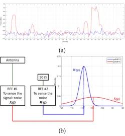
The level ofW(f)can be obtained by replacing the Winegard antenna with a 50Ω load and taking measurements for this load, to register the noise of the system at that precise instant of time [20]. The 50Ω load corresponds to the input impedance of the RF-Explorer (RFE) used to sense the noise signal [35].

For this research, we decided to use this second option, adding an extra RFE device with a 50Ωload attached to the main RFE that senses the TV signal.

In Figure 3.2 are illustrated both signals sensed and plotted together, the noise and the composed signal plus noise, collected with a RFE and Spectrum Analyzer (SA) respectively.

(a) (b)

FIGURE3.2: Overlapped plots for the composed signal in red and noise in blue, (a) for RFE and (b) for SA.

3.1.3 Additional Considered Parameters

With the purpose of ensuring the PU detection, additional parameters had been considered. First is the pilot tone which can be found in specific frequencies of the channel. Second is the information obtained from an external source. And third, a TV device attached to the SSS.

Pilot Detection (PD)

The pilot tone of a TV channel usually is located at a frequency of 310KHz ±

(35)

channel, it is possible to collect the samples, the device then jumps to the next channel by increasing 6MHz to the sampled frequency, when it reaches channel 51 (592.310MHz), it returns to channel 19 (500.310MHz) and repeats the cycle. If a pilot tone was detected, that channel was considered as a potentially used.

FIGURE 3.3: Pilot tone detected in channel 20 (506.31MHz ± 100KHz).

Information from an External Source

In this case, it is a database (DB) of the channels, frequencies, and signal strength available in the city of Windsor, according to an authorized provider. Addi-tionally, we use the information of those channels received and decoded by a conventional TV receptor attached to the SSS. The channels with enough nom-inal reception power, are considered as TV Black Spaces (TVBS), and its use is banned. Results of theE(f)are displayed in Table 3.1.

(36)

TABLE3.1: Active TV channels received in Windsor area.

Channel Sub-channel Type Station/Network

20

1 HD WYMD-HD

2 SD WMYD-AT

3 SD WMYD-ES

26 1 HD CHWI

31

1 HD ION

2 SD QUBO

3 SD IONLIFE

4 SD SHOP

5 SD QVC

6 SD HSN

32 1 HD TVO

38

1 HD WADL-HD

2 SD GRIT

3 SD GET TV

4 SD COZI TV

5 SD THE WORD

6 SD JUSTICE

7 Audio 910 AM

50 1 HD WKBD-HD

TV Decoded Signal Visualization Device

It consists of a TV set connected to the receptor antenna of the SSS. Its purpose is to visualize the decoded signal of the received channels. In other words, it is used to verify the real reception of the TV stations that are mentioned as active in the DB of the previous point, as a redundant resource to ascertain the presence of PU.

3.2 Designing a Spectrum Sensing Station

(37)

FIGURE3.4: Proposed SSS to sense spectrum in indoor and out-door fixed locations.

Figure 3.4 shows a diagram for the SSS, it has three versions: A fixed SSS, for outdoor spectrum sensing, a portable SSS for indoor spectrum sensing, and a M-SSS, Figure 3.5 shows the portable version for indoor use. For implement the SSS the components described below were used.

Hardware

• Antenna Winegard, model MS-3005 VHF/UHF, 14.9".

• 3-way satellite TV splitter, 5MHz to 2050MHz, F - female connectors, 75Ω nom. impedance.

• Spectrum Analizer Tektronix MDO4054-3.

• RF Explorer Sub1G.

• RTL SDR 2832U.

• DELL laptop, Intel i-5-5200U CPU @ 2.20GHz, RAM 6GB, 64-bits OS.

Software

• RF Explorer for Windows, Version v1.23.1711 - for use with firmware v1.23.

• AIRSPY Windows SDR Software Package.

• Matlab Student version 2017.

• CubicSDR v0.2.2- OS X.

• Gqrx Mac OS X 10.11.

(38)

3.2.1 Spectrum Analyzer Tektronix MDO4054-3

It is an oscilloscope with a built-in spectrum analyzer, made by Tektronix [37], it permits to capture time-correlated analog, digital, and RF signals.

SA Technical characteristics

• Frequency Range 50KHz to 3GHz.

• Bandwidth 500MHz.

• Span 1KHz to 3GHz.

• Frequency Resolution 20Hz to 10MHz.

• Average Noise Level -115dBm.

• Amplitude Resolution 0.5dBm.

• Automatic RBW 2.6KHz to 600KHz.

• Price: $7,950.00CAD.

3.2.2 RF Explorer Sub1G

RF Explorer is a portable spectrum analyzer designed for the specific needs of digital radio frequency communication. It is able to display full frequency spectrum in the band, existed spread spectrum activity, bandwidth to monitor collisions, and frequency deviation from the expected tone, etc. The workflows are supported by RF Explorer, which include detection of expected transmission and power, automatically resolving Resolution Bandwidth (RBW) and sweep time and spectrum data calculations. Moreover, real-time or adjusted signals, 3D spectrogram waterfall, Comma-Separated Values (CSV) export, high-quality graphics, and a large feature set can be performed through cooperated work between RFE and Windows on PC [35].

RFE Technical characteristics

• Frequency Range 240MHz to 960MHz.

• Span 0.112MHz to 300MHz.

• Frequency Resolution 1KHz.

(39)

• Amplitude Resolution 0.5dBm.

• Automatic RBW 2.6KHz to 600KHz.

• Price: $198.13CAD.

NooElec RTL-SDR is an inexpensive software define radio hardware which supports wide variance of the cross-platform Operative System (OS), for exam-ple, OS10, Windows 32 & 64 bit, MacOS, Linux etc. It uses USB Interface IC RTL2832U and Tuner IC R820T2. We have used a sampling rate of 2.56MHz, which is 80% of the resources of the SDR. Due to its modulation techniques, it is easy and quick to identify the type of signal is broadcasting. Moreover, it shows how the waveform changes. It is a simple handy to find the signal and decode the information and does not use the whole bunches of resources [38], [39].

Technical characteristics

• Sample rate from 250KHz up to 3.2MHz.

• Modulation techniques: FM, FMS, NBFM, AM, LSB, USB, DSB & I/Q.

• Audio sample rate 44.1KHz to 96KHz.

• Frequency range is 25MHz to 1750MHz.

• Price: $ 40.95CAD.

(40)

3.3 Designing a Mobile Spectrum Sensing Station

With the SSS implemented and its functionality tested using the fixed and portable antennas, it is necessary to design a mobile version to obtain information of the spectrum in the city, by mounting it in a vehicle to cover broad areas.

FIGURE 3.6: Initial diagram for the M-SSS, designed to be mounted in a vehicle and sense the TV spectrum in wide

geo-graphical areas.

As observed in Figure 3.2, both devices, the SA and RFE detect energy in the UHF TV band, the only difference is the number of samples taken by each device, but in general, they are able to detect the presence or absence of a PU.

With this in mind, the M-SSS originally was designed as is shown in Figure 3.6, using a Winegard antenna, only one RFE device, a portable computer and a storage device to save the collected data. For this mobile configuration, it is mandatory to attach a Global Positioning System (GPS) antenna to collect the geographical location for each reading.

The M-SSS works mounted in a moving vehicle, to reach this, a support was assembled using Chlorinated Polyvinyl Chloride (CPVC) pipes, it was designed to fit in a Dodge Grand Caravan vehicle, as is shown in Figure 3.7, where (a) is the design draft, (b) the M-SSS mounted, (c) the supporting structure built with CPVC, (d) the support mounted in the vehicle, (e) Winegard and GPS antennas, and (e) the M-SSS collecting data.

(41)

(a) (b)

(c) (d)

(e) (f)

FIGURE 3.7: M-SSS (a) design diagram, (b) station mounted, (c) supporting structure built in CPVC, (d) supporting installed in the vehicle, (e) Winegard and GPS antennas, and (f) M-SSS in

opera-tion.

3.4 Data Collection Procedure

(42)

3.4.1 Fixed Data Collection

Samples were collected in the Centre for Innovation and Engineering (CEI) building, located in the city of Windsor, coordinates (Latitude 42.3044 N, Longi-tude -83.061263 W). The Winegard antenna, model MS-3005 was installed on the roof of the building it means about 12 meters height over the city, which has an altitude of 190 meters above sea level. Measurements were taken several times at different hours of the day and in different periods of time. The radio-electric signals received by the omnidirectional antenna were carried by the coaxial ca-ble to the 3-way splitter input, in the outputs, the RF signal theoretically has the same attenuation level, it was feed into the different Data Acquisition In-strument (DAI) to ensure similar electromagnetic characteristics of the sampled signal. With this parallel feed, the lecture of the different DAI can be compared, due to the similarity of the analyzed signals.

Sensing Procedure

Using the RFE, a single reading of the UHF TV spectrum obtains 112 samples, the RFE can take a reading every 0.340s, the plot of a single reading is repre-sented in Figure 3.8 using a blue line. When the reading is made with the SA, this device obtains 1005 samples. The collected information of 198MHz band-width is represented in Figure 3.8 using a red line.

Comparing the overlapped plots, the general shape of the spectrum energy is observed without major variations. This interesting fact, give us the possibil-ity to use the RFE device to replace the voluminous, heavy, and costly SA.

(43)

FIGURE 3.8: TV Signal sensed an RFE (blue line) and a SA (red line) are compared. The general shape that contains the energy is

easily identified in the plot obtained with both devices.

Comparing the DAI Performance

Three different DAI are combined in the designed SSS, to know the character-istics of each device, a performance comparison is needed. In Table 3.2 are de-tailed the DAI, the sensing technique, the whole 198MHz bandwidth, the num-ber of channels sensed, and the performance observed when each device was used.

The SA, an expensive and accurate device has a high performance to sense the whole bandwidth of 32 TV channels or a single 6MHz channel, with this DAI is possible to apply the ED and the PD techniques simultaneously.

Using the RFE, when it senses all the 198MHz band, it only can detect the energy of the TV channels but is not able to detect the pilot tones of the 32 channels sensed at time, on the other hand, if it senses only one 6MHz channel, its performance increases and can detect both, the energy and pilot presence in a single TV channel.

(44)

TABLE3.2: DAI’s features and performance comparison

DAI ED PD Bandwidth # Channels Performance

SA 198 MHz 32 High

SA 6 MHz 1 High

RFE N/A 198 MHz 32 Medium

RFE 6 MHz 1 High

RTL N/A N/A 198 MHz 32 N/A

RTL N/A 3 MHz 0.5 High

3.4.2 Mobile Data Collection

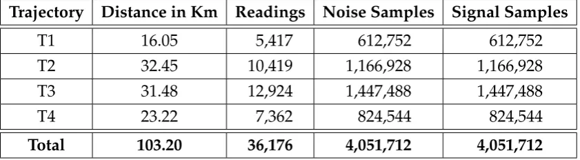
To sense the TV spectrum data in the city of Windsor using the M-SSS, four tra-jectories were defined, as is illustrated in Figure 3.9. In total more than 36,176 readings or 4,051,712 samples for noise and 4,051,712 samples for the composite signal plus noise were taken. From these readings, 53 points distributed across the city were selected to plot the information obtained. The trajectories are de-tailed in Table 3.3.

FIGURE 3.9: Trajectories and locations to represent the TV spec-trum sensed in the city of Windsor.

(45)

TABLE 3.3: Trajectories defined to sense the TV spectrum in the city of Windsor

Trajectory Color Initial Point Final Point Observations

1 Red 1 10 10 Points

2 Purple 11 27 17 Points

3 Blue 28 48 21 Points

4 Orange 49 53 5 Points

Total 53 Points

As is mentioned above, in Figure 3.9, the coloured line represents the trajec-tories followed by the M-SSS and blue circles represent the points in which the data are plotted and analyzed. It is necessary to note that all the time during the movement of the M-SSS along the trajectories the information is saved in the DB, Figure 3.10 illustrates how the TV signal contained in the 198MHz band is saved, and in this case, visualized by using the RFE software [35].

FIGURE3.10: Visualization of the TV signal sensed using an RFE device, the readings were taken every 0.340s, the axis represents

(46)

Chapter 4

Stochastic Analysis of TVWS

As mentioned in the objectives of the research, a model based on the proba-bilistic characteristics of the sensed signal needs to be developed for identifying TVWS. This model and the mechanism of finding TVWS are described in this chapter. Additionally a table with a mathematical notation and units of mea-surement has been included in Appendix B.

4.1 Sensing the TV Signal

The existence of the PU can be verified by using the following hypotheses:

H0 : X(f) =W(f) (4.1)

H1 : X(f) =S(f) +W(f) (4.2)

where W(f) denotes Additive White Gaussian Noise (AWGN), S(f) is the re-ceived signal of the PU,X(f)is the sensed signal, andH0represents the absence

of PU over the channel, whereas H1represents the presence of the PU over the

channel.

By using the SSS, the information from the UHF TV spectrum was collected at each instant of timetiand plotted as is shown in Figure 4.1. In both cases, (a)

(47)

(a)

(b)

FIGURE4.1: TV Signal sensed with (a) RFE and (b) SA are com-pared. The general shape that contains the energy under the red

line is easily identified in both devices.

With only the information ofX(f)is not enough to identify TVWS, it is ev-ident that more data is needed to find them. So it is mandatory to find more parameters that permit to detect the presence of PU.

4.2 Identifying the Noise Level

A crucial element to be considered is how the noise is measured, and the mean of the noise W(f) is calculated. In some cases, the noise is sensed at the begin-ning of the measurement campaign and that value is used to be compared with all the readings. In other cases, a theoretical value is considered. Again a third approach is to consider a fixedT, we can recallTis the threshold. In practice, it is very difficult to obtain accurate information about the noise power [40].

According to the IEEE 802.22 standard [4], [17], the channel in operation must be sensed several times, namely, during the transmission, inter-framing and in-framing. Here, it is important to obtain trustful and accurate channel noise and signal samples.

(48)

the signal X(f) is received through the antenna and sensed with one DAI, and at the same time, another DAI of similar characteristics with a 50Ω matched impedance is used to sense the noise of the system. As a result, both the signals, i.e., X(f)andW(f)are used in our proposed channel sensing mechanism.

FIGURE 4.2: Proposed M-SSS to sense in parallel the NoiseW(f)

and the composite signalX(f).

With the above-mentioned configuration, the UHF TV spectrum was sensed, and the obtained results are shown in Figure 4.3.

(a)

(b)

FIGURE 4.3: TV Signal sensed with (a) RFE and (b) SA are com-pared. The W(f) and X(f) are observed and permit infer their

possible relationship.

(49)

W(f)and that indicates the real noise level at an instantti. This is the reference

level for calculatingT.

(a)

(b)

FIGURE4.4: TV Signal sensed with (a) RFE and (b) SA are com-pared. The W(f)andX(f)are observed and it is considered the

noise level for that specific data collected.

4.3 Threshold Considerations

As found in the literature of TVWS sensing, the sensed signalX(f)is compared withT, which is obtained from

T =W(f) +M (4.3)

where W(f)is the mean of the noise. Here Mis a margin that can be calculated from different manners and is a crucial element to consider a channel as a TVWS [20].

Literature shows different values of M have been used in the past. For ex-ample, [41] considered an Mof 5dB, [42] used a value of 7dB. Again as far ITU recommendation the value of Mshould be 10dB [43]. Finally, in [44], a fixed T

(50)

(a)

(b)

FIGURE4.5: Comparison of the signal sensed with (a) RFE and (b) SA. In both sub-figures are plottedX(f), W(f), and the different

values forMorT.

In Figure 4.5 we can observeX(f), sampled with RFE in (a) and with SA in (b). Both the sub-figures show the previously discussed MandT. It is obvious from these figures that the higher is the chosen value of M, the higher is the occurrence of signal missed-detection.

In the specific case of T = -78dBm, all the 32 channels appears to be idle; which is not necessarily true because at least 8 signal peaks can be observed.

The purpose of sensing and plotting two signals, i.e.,W(f) and X(f) is to identify the characteristics of each signal and compare with the other. This will permit to obtain enough parameters to develop the proposed probabilis-tic model.

The above discussion reveals that in order to sense the UHF TV spectrum for accurate identification of idle channels, it is imperative to define an adaptiveT. The value of Tshould satisfy the following conditions.

(i) It should be close enough from W(f)to avoid missed-detection.

(ii) It should be far enough from W(f)to avoid false alarms.

(iii) It should be adaptive to the possible changes experienced by W(f) and

(51)

4.4 Probabilistic Considerations

4.4.1 Working with Normal Distributions

As mentioned earlier, two signals, i.e., the noiseW(f)and the composite signal plus noiseX(f) are collected simultaneously by the RFE devices connected in parallel. It is imperative to verify that the sensed noiseW(f)is a normally dis-tributed signal. There are two ways to do this, i.e., graphical and mathematical methods [45], [46]. The first one considers graphical methods where the sam-ples of the noise signal are plotted to observe the distribution. Following this method, Figure 4.6(a) shows the histogram of noise samples taken in a particu-lar location and Figure 4.6(b) shows the normal probability distribution plot of the same samples. It is visually evident that the plotted samples correspond to a normal distribution.

(a) (b) (c)

FIGURE4.6: Noise signal sensedW(p). (a) Histogram of the col-lected data. (b) Normal probability plot of the same data read. (c)

CDF of the Kolmogorov-Smirnov Test (KST) applied.

The second method is a mathematical test; in this case, the Kolmogorov-Smirnov Test (KST) [46]. This test with a significance level of 5% has been ap-plied to the collected noise samples, and the corresponding results of the Cu-mulative Density Function (CDF) are shown in Figure 4.6(c). The plots suggest that the tested samples are normally distributed.

On the other hand, as shown by Figures 4.7(a) and (b), the composite signal

(52)

(a) (b) (c)

FIGURE 4.7: Composite signal plus noise sensed Xo(p). (a) His-togram of the collected data. (b) Normal probability plot of the distribution for the same reading (c) CDF of the

Kolmogorov-Smirnov Test (KST) applied.

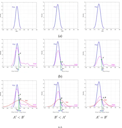
To apply the proposed model, it is necessary to assume that the composed signal X(p) is a normally distributed signal, as illustrates Figure 4.8. This as-sumption is needed in order to reduce the computational complexity in terms of probabilistic analysis while accuracy is preserved in the TVWS identification procedure.

(a) (b) (c)

FIGURE4.8: The curveXo(p)of the multi-modal distribution of (a) can be assumed as the normal distribution curve X(p)of (b), this assumption summarized in (c) allow us to reduce the calculation

complexity of the proposed model.

In Figure 4.9 are plotted the pdfs ofW(p) in blue,Xo(p)in magenta, which is the multi-modal curve of the composite signal, and X(p)in red. In these fig-ures, it is easy to observe that the intersections ofW(p)∩X(p)andW(p)∩Xo(p)

(53)

(a)

(b)

A0 <B0 B0 < A0 A0 = B0

(c)

FIGURE4.9: Readings taken in three different points, the pdf for the noise W(p)is plotted in blue, multi-modal composite signal Xo(p)in magenta, and composite signal X(p) in red. In (a) are shown the pdf of the noise for each location. In (b), the intersection point "A" ofW(p)∩Xo(p)and its projection to the power axis "A0". In (c), the intersection point "B" ofW(p)∩X(p), and its projection to the power axis "B0", we also observe that the difference between A0 andB0 is minimum concerning the power level of the signal in

dBm.

Now, this assumption is supported by the fact that the calculation of the Probability of False Alarm (Pf a) will be done on the noise signal, i.e., W(p),

which corresponds to a normal distribution.

(54)

(i) For calculation ofPf a, the left intersection point"C"of the pdf ofW(p)and

X(p)will not be considered, because it is located below the mean value of the noise signal W(p).

(ii) For calculation of the Probability of Detection (Pd), the right intersection

point"B"of the pdf ofW(p)andX(p)will be considered.

Once this assumption has been accepted, then the pdf that represent the noiseW(p)and the composite signalX(p)are those illustrated in Figure 4.10.

FIGURE 4.10: Normal distribution pdfs forW(p)in blue and as-sumed X(p)in red, both used to calculate the Pf a and the Pd

ac-cording to the model proposed in this dissertation.

In this point, it is precise to refer to the Neyman-Pearson article, namedOn the Problem of the Most Efficient Tests of Statistical Hypotheses [47]. The authors used Fisher’s null hypothesis significance testing [48] and the p-value as part of a formal decision process. Thus, they raised a real choice between two rival hypotheses. The hypothesis contrast became a method to distinguish between the null hypothesis and the alternative hypothesis, as observed in Figure 4.11.

In the proposed model, the pdf of the composite signal contains the pdf of noise, while in the Neyman Pearson model, both pdf are partially overlapped. On the other hand, the Pf aand Pdare similarly defined and related.

The frequently used statistical parameters regarding the sensed signals are

Pf a, Pd, and the probability of missed-detection (Pm). With the collected

infor-mation ofW(p)and X(p), and considering that both signals correspond to nor-mal distributions, other statistical parameter can be calculated, i.e., mean values of the signals (W(p), X(p)) or the standard deviations (σW, σX). An

(55)

FIGURE4.11: Neyman Pearson model, the null hypothesis and the alternative hypothesis are observed.

which provides a visual explanation of the proposed method, and is explained next.

To plot the pdf of a signal that responds to a normal distribution, it is neces-sary to apply

f(x) = 1 σ √ 2π exp ( −1 2

x−x(p) σ

2)

; −∞ <x <∞ (4.4)

whereσ is the standard deviation and x(p) is the mean of the distribution. By

taking the samples ofW(p)andX(p), the equations that define both pdf curves, are f(xW) and f(xX)with W(p)and X(p)as the means,σW andσX as the

stan-dard deviations respectively, then the equations be:

f(xW) =

1 σW √ 2π exp ( −1 2

x−W(p) σW

2)

(4.5)

f(xX) = 1

σX √ 2π exp ( −1 2

x−X(p) σX

2)

(4.6)

now, considering that X(p) is a composite signal consisting of W(p) + S(p), whereS(p) is the energy of the PU andW(p)is the noise, it is very important to compare both pdf.

4.4.2 Obtaining pdfs

RFE Device

(56)

noise W(p), standard deviation of the composite signalσX, and standard

devi-ation of the noiseσW are calculated and used to plot the pdfs as shows Figure

4.12(a).

SA Device

Repeating the same procedure used for RFE device, now using the SA, 1005 samples are collected, and then after calculating the mean and the standard deviation, the pdfs are plotted as illustrated in Figure 4.12(b).

(a) (b)

FIGURE4.12: Pdf ofW(p)in blue andX(p)in red, taken from the data collected with (a) RFE and (b) SA.

4.4.3 Performance Metrics

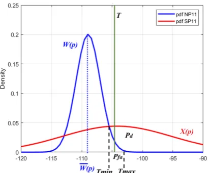
In order to visualize the performance metrics of spectrum sensing, i.e., probabil-ity of false alarm, probabilprobabil-ity of detection and probabilprobabil-ity of missed-detection, we need to consider the pdf curves andTtogether as shown in Fig. 4.13.

Probability of False Alarm: Pf a

Pf a refers to the probability that a peak or peaks of the noise signal is detected

above T, and is considered as a real signal of the PU when in reality no PU signal is present. In Figure 4.13, Pf a corresponds to the area bounded by Tand

(57)

Probability of Detection:Pd

Pd is the probability that a real signal of the PU is detected above T, and is

considered as a signal from PU. In Figure 4.13 it refers to the area bounded by

TandX(p)coloured with yellow.

Probability of Missed-Detection: Pm

Pm is the probability that a real signal of the PU is not detected above T, and is

considered as noise due to its low amplitude. In Figure 4.13 it is colored with light-blue.

FIGURE4.13: Graphical representation of thePm,Pf a, andPd,

gen-erated by theTand the pdf curves forW(p)andX(p).

4.4.4 Calculation of Threshold

T

In light of the previous discussion, it is evident that T is the most critical pa-rameter for accurate sensing, and hence it must be meticulously calculated to permit the balance ofPf a and Pd. By obtaining Man adequate T can be

calcu-lated. Basically, M is the product of the standard deviationσ and the value of z.

It is possible to define a minimum limit Mmin and a maximum limit Mmax

(58)

FIGURE4.14: Minimum and maximum possible values forM.

In other words,M must remain between the maximum and minimum pos-sible values.

Mmin ≤ M≤ Mmax (4.7)

where Mmin is obtained calculating the intersection point of two plotted pdfs.

Mmin =W(p)∩X(p) (4.8)

which is a complex operation considering Equations 4.5 and 4.6. The value of Mmaxis calculated using

Mmax =σz (4.9)

whereσis the standard deviation of the distribution andzis obtained from the F(z)function, which defines the area under the curve in terms of the standard deviation [49].

Spectrum Occupancy Estimation and Analysis