Optimization of the SHiP Spectrometer Tracker geometry
1using the Bayesian Optimization with Gaussian Processes
2OlegAlenkin1,MikhailHushchyn1,2,∗,AndreyUstyuzhanin2,3, andAlexanderBaranov2,3
3
1Skolkovo Institute of Science and Technology
4
2National Research University Higher School of Economics
5
3Yandex School of Data Analysis
6
Abstract.One of the most important aspects of data processing at SHiP [1] ex-7
periments is tracks pattern recognition. The purpose of the SHiP Spectrometer 8
Tracker (SST) is efficient reconstruction of charged particle tracks originating 9
from decays of neutral New Physics objects. The reconstruction performance 10
strongly depends on the tracker design and should be considered as an objective 11
to define the best SST geometry parameters. In this study the SHiP Spectrom-12
eter Tracker geometry optimization using Bayesian optimization with Gaussian 13
processes in considered. The study have been done on MC data. The first results 14
of the optimization are also considered. 15
1 Introduction
16SHiP is a fixed-target experiment at the CERN SPS accelerator proposed recently for searches 17
of the hidden particles predicted by a variety of physics models beyond the Standard Model 18
[1, 2]. The purpose of the SHiP Spectrometer Tracker (SST) is efficient reconstruction of
19
charged particle tracks originating from decays of neutral New Physics objects. The SST 20
geometry parameters have to be optimized to achieve the highest reconstruction efficiency.
21
One of the most popular methods of optimization is grid search. The disadvantage of 22
this method is exponential grid size growth with increase of the number of optimization 23
parameters. This requires large computational resources to check all grid nodes. In the 24
SST geometry optimization task, evaluation of every node requires large statistics Monte 25
Carlo simulation of SHiP physics events, what makes the grid search approach too expensive. 26
Bayesian optimization method [3] is well-suited to the optimization of expensive objective 27
functions. Using information from all previously evaluated nodes, the method chooses the 28
next node to be checked requiring the objective function to have larger probability for the 29
optimum. This allows to find the optimum with lower number of checks than with the grid 30
search. 31
Bayesian optimization method was tested in our previous study on simulator tuning [4] 32
and showed promising result. In this study the SHiP Spectrometer Tracker geometry opti-33
mization using the Bayesian optimization with Gaussian processes (GP) [3, 5] is considered. 34
Decay Spectrometer
– surround background tagger – straw spectrometer– EM calorimeter – Timing detector – Muon detector
0 background
=
⇒
2 candidates are a discovery
measure candidates mass and identify final state
=
⇒
narrow down physics models
decay
volume
redesigned
8 / 17
Target and Hadron Absorber
Scattering and Neutrino Detector
Spectrometer Tracker p
HNL
𝝁𝝁
𝝅𝝅
Figure 1: The SHiP detector.
2 SHiP Spectrometer Tracker
35
SHiP [6, 7] experiment was proposed in 2013 for searches of weakly interacting long-lived
36
particles predicted by the Hidden Sector theoretical models. The general scheme of the
de-37
tector is demonstrated in Fig. 1. SHiP is a detector with a fixed target. A proton beam from
38
the CERN SPS accelerator with energy of 400 GeV bumps into it. The target [8] is designed
39
to maximize production of charm and beauty hadrons and photons. It is followed by the 5m
40
hadron absorber that absorbs all particles except weakly interacting ones: muons, neutrinos,
41
and particles of new physics. The Muon Shield [9, 10] is used to reduce muon flux in the
42
detector acceptance. The shield is a system of 6 magnets with a total length of 35m. The
av-43
erage magnetic field is 1.7T. The Scattering and Neutrino Detector (SND) [11, 12] is located
44
after the muon shield. The goal of the detector is to study neutrino physics and to detect light
45
dark matter candidates.
46
SND is followed by the second detector complex [11] for studying visible decays of the
47
Hidden Sector particles — Heavy Neutral Leptons (HNL). The complex consists of the
De-48
cay Volume, Spectrometer Tracker, Electromagnetic Calorimeter and Muon Detector. HNL
49
decays in the Decay Volume into visible particles. Fig. 1 shows an example of theHNL→µπ
50
decay. The spectrometer is used to reconstruct the tracks of the visible particles. The
Elec-51
tromagnetic Calorimeter and the Muon Detector are used to identify their types.
52
The SHiP Spectrometer Tracker has 2 straw tube stations before the magnet and 2 stations
53
after it. Each station has 4 views: 2 Y-views with straw tubes oriented parallel to X-axis and
54
U, V-views rotated by a small angle,+αor−α, around the Z axis. A view has 2 planes with
55
2 straw tubes layers in each plane as it is shown in Fig 2. The view geometry defines the
56
particle track recognition [13] quality. The geometry is defined by the following parameters:
57
straw pitch, Z shift between layers, Z shift between planes, Z shift between views, Y offset
58
between layers, Y offset between planes and angleαbetween Y and U, V views. The goal of
59
this study is to find optimal values of these parameters.
60
∗e-mail: [email protected]
Decay Spectrometer
– surround background tagger – straw spectrometer– EM calorimeter – Timing detector – Muon detector
0 background
=
⇒
2 candidates are a discovery
measure candidates mass and identify final state
=
⇒
narrow down physics models
decay
volume
redesigned
8 / 17
Target and Hadron Absorber Scattering and Neutrino Detector Spectrometer Tracker p HNL 𝝁𝝁 𝝅𝝅
Figure 1: The SHiP detector.
2 SHiP Spectrometer Tracker
35
SHiP [6, 7] experiment was proposed in 2013 for searches of weakly interacting long-lived
36
particles predicted by the Hidden Sector theoretical models. The general scheme of the
de-37
tector is demonstrated in Fig. 1. SHiP is a detector with a fixed target. A proton beam from
38
the CERN SPS accelerator with energy of 400 GeV bumps into it. The target [8] is designed
39
to maximize production of charm and beauty hadrons and photons. It is followed by the 5m
40
hadron absorber that absorbs all particles except weakly interacting ones: muons, neutrinos,
41
and particles of new physics. The Muon Shield [9, 10] is used to reduce muon flux in the
42
detector acceptance. The shield is a system of 6 magnets with a total length of 35m. The
av-43
erage magnetic field is 1.7T. The Scattering and Neutrino Detector (SND) [11, 12] is located
44
after the muon shield. The goal of the detector is to study neutrino physics and to detect light
45
dark matter candidates.
46
SND is followed by the second detector complex [11] for studying visible decays of the
47
Hidden Sector particles — Heavy Neutral Leptons (HNL). The complex consists of the
De-48
cay Volume, Spectrometer Tracker, Electromagnetic Calorimeter and Muon Detector. HNL
49
decays in the Decay Volume into visible particles. Fig. 1 shows an example of theHNL→µπ
50
decay. The spectrometer is used to reconstruct the tracks of the visible particles. The
Elec-51
tromagnetic Calorimeter and the Muon Detector are used to identify their types.
52
The SHiP Spectrometer Tracker has 2 straw tube stations before the magnet and 2 stations
53
after it. Each station has 4 views: 2 Y-views with straw tubes oriented parallel to X-axis and
54
U, V-views rotated by a small angle,+αor−α, around the Z axis. A view has 2 planes with
55
2 straw tubes layers in each plane as it is shown in Fig 2. The view geometry defines the
56
particle track recognition [13] quality. The geometry is defined by the following parameters:
57
straw pitch, Z shift between layers, Z shift between planes, Z shift between views, Y offset
58
between layers, Y offset between planes and angleαbetween Y and U, V views. The goal of
59
this study is to find optimal values of these parameters.
60
∗e-mail: [email protected]
Layer 2 Layer 1 Layer 2 Layer 1
Plane 1 View Plane 2
zshift_plane
yoffset_plane
zshift_layer yoffset_layer pitch
Figure 2: The SHiP Spectrometer Tracker stations and an example of HNL decay (left). The view layout and parameters for optimization (right).
3 Gaussian Processes Regression
61
GP regression [3, 5] is used for the spectrometer geometry optimization as described in the
62
next section. Consider an objective functiony= f(x) and a set of observations{xi, yi}ni=1. In 63
the GP concept, the sequence of observations can be represented as a sample from a Gaussian
64
distribution:
65
y=(y1, y2, ..., yn)T ∼ N(0,K) (1)
whereN(0,K) represents multivariate Gaussian (or normal) distribution with zero mean
66
and covariance matrixK. For a new point (xn+1, yn+1) a similar relation with the new covari-67
ance matrixK
can be written:
68
y yn+1
∼ N(0,K) (2)
where the covariance coefficientski jcharacterize the correlation between different points
69
of the process: for nearby points xiandxjthe observablesyiandyjare strongly correlated
70
than for distant points. Here squared exponential covariance function is used to define
coef-71
ficientski j:
72
K=
K k
kT k(xn+1,xn+1)
, k=
k(x1,xn+1) k(x2,xn+1)
.. . k(xn,xn+1)
, k(xi,xj)=exp(− 1
2θ2xi−xj 2
) (3)
whereθdefines the smoothness of the objective function.
73
The mean and standard deviation of the objective function approximation, µ(xn+1) and 74
σ(xn+1), are defined by the conditional distribution: 75
(yn+1|y)∼ N(µ(xn+1), σ(xn+1)) (4)
µ(xn+1)=kTK−1y (5)
σ(xn+1)=k(xn+1,xn+1)−kTK−1k (6)
The optimalθvalue in the covariance matrixKis found based on the likelihood function 76
optimization: 77
θopt=arg max
θ logp(y|X, θ) (7)
logp(y|X, θ)=−1
2yTK−1y− 1
2log|K| − n
2log 2π (8)
Equations forµ(xn+1) andσ(xn+1) are used during Bayesian optimization to approximate
78
the objective function based on known observations. 79
4 Bayesian Optimization
80Bayesian optimization [3] is a method of finding the optimum of an expensive objective 81
function. The goal of the Bayesian optimization is to find the optimum using an as small as 82
possible number of function calculations. The Bayesian optimization loop has the following 83
steps which are repeated until the optimum is found: 84
• Given observations{xi, yi= f(xi)}ni=1, fit a GP regression model to getµ(xn+1) andσ(xn+1)
85
of the objective function approximation. 86
• Optimize the Expected Improvement (EI) acquisition function [14] based on the regression model for sampling the next point:
xn+1=arg max
x EI(x)
EI(x)=E[max{0,f(x−)−fˆ(x)}], fˆ(x)∼ N(µ(x), σ(x)), x−=arg min
xk∈{xi}ni=1 f(xk)
• Sample the next observation (xn+1, yn+1= f(xn+1)).
87
5 SHiP Spectrometer Tracker Optimization
88The goal of this study is to find the optimal geometry of the SHiP Spectrometer Tracker us-89
ing Bayesian optimization with GP. The parameter values of the SHiP Spectrometer Tracker 90
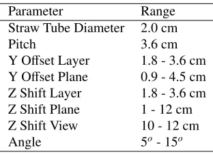
geometry used during the optimization are listed in Tab. 1. 91
Parameter Range
Straw Tube Diameter 2.0 cm
Pitch 3.6 cm
Y Offset Layer 1.8 - 3.6 cm
Y Offset Plane 0.9 - 4.5 cm
Z Shift Layer 1.8 - 3.6 cm Z Shift Plane 1 - 12 cm Z Shift View 10 - 12 cm
Angle 5o- 15o
Table 1: Geometry parameter ranges for the optimization.
σ(xn+1)=k(xn+1,xn+1)−kTK−1k (6)
The optimalθvalue in the covariance matrixKis found based on the likelihood function 76
optimization: 77
θopt=arg max
θ logp(y|X, θ) (7)
logp(y|X, θ)=−1
2yTK−1y− 1
2log|K| − n
2log 2π (8)
Equations forµ(xn+1) andσ(xn+1) are used during Bayesian optimization to approximate
78
the objective function based on known observations. 79
4 Bayesian Optimization
80Bayesian optimization [3] is a method of finding the optimum of an expensive objective 81
function. The goal of the Bayesian optimization is to find the optimum using an as small as 82
possible number of function calculations. The Bayesian optimization loop has the following 83
steps which are repeated until the optimum is found: 84
• Given observations{xi, yi= f(xi)}ni=1, fit a GP regression model to getµ(xn+1) andσ(xn+1)
85
of the objective function approximation. 86
• Optimize the Expected Improvement (EI) acquisition function [14] based on the regression model for sampling the next point:
xn+1 =arg max
x EI(x)
EI(x)=E[max{0,f(x−)−fˆ(x)}], fˆ(x)∼ N(µ(x), σ(x)), x−=arg min
xk∈{xi}ni=1 f(xk)
• Sample the next observation (xn+1, yn+1= f(xn+1)).
87
5 SHiP Spectrometer Tracker Optimization
88The goal of this study is to find the optimal geometry of the SHiP Spectrometer Tracker us-89
ing Bayesian optimization with GP. The parameter values of the SHiP Spectrometer Tracker 90
geometry used during the optimization are listed in Tab. 1. 91
Parameter Range
Straw Tube Diameter 2.0 cm
Pitch 3.6 cm
Y Offset Layer 1.8 - 3.6 cm
Y Offset Plane 0.9 - 4.5 cm
Z Shift Layer 1.8 - 3.6 cm Z Shift Plane 1 - 12 cm Z Shift View 10 - 12 cm
Angle 5o- 15o
Table 1: Geometry parameter ranges for the optimization.
Figure 3: The maximal value of the objective function defined as the number of reconstructed track per a generated event, as a function of the number of iterations.
(a) (b)
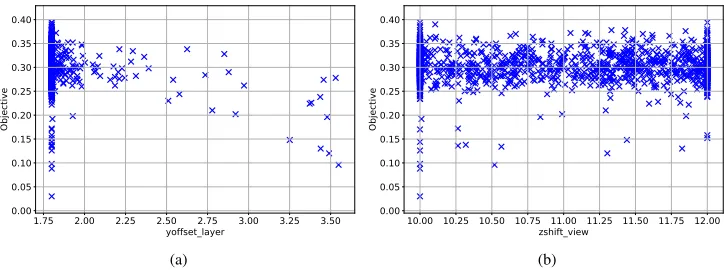
Figure 4: Dependencies of the objective function from (a) Y offset between layers and (b) Z
shift between views for observations of the optimization.
For each combination of the parameters a set of 500 events of HNL → µπdecay is 92
generated using FairShip [15]. Then, a track pattern recognition algorithm [11] is applied 93
to find tracks based on hits in the spectrometer. The simulation and recognition for one 94
combination of the parameters takes about 1000 seconds. For the optimization the following 95
objective function is calculated: 96
Ob jective=Nrecognized tracks
Ngenerated events
whereNrecognized tracksis number of recognized tracks in 500 events;Ngenerated events=500
97
is number of events. Bayesian optimization with GP realized in GPy [16] python library is 98
used to maximize the objective function. The found objective maximum after each iteration 99
of the optimization is shown in Fig. 3. The optimization shows that Y offsets between straw
100
tubes layers and planes of the spectrometer have the greatest impact on the objective function 101
as it is shown in Fig. 4a. They have optimal values of 0.5×Pitch=1.8 cm and 0.25×Pitch=
102
0.9 cm respectively. The smaller Z shift between layers the better, but there are no significant 103
(a) (b)
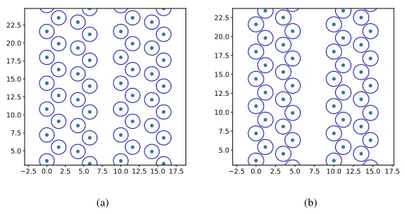
Figure 5: Straw tubes of two views for baseline (a) and optimized (b) geometries.
YO
ff
set
Layer
YO
ff
set
Plane
Z
Shift
Layer
Z
Shift
Plane
Z
Shift
V
ie
w
Angle
Baseline 1.9 cm 1.3 cm 1.6 cm 4.4 cm 10 cm 5o
Optimized geometry 1.8 cm 0.9 cm 1.2 cm 3.5 cm 10 cm 5o
Table 2: Values of the spectrometer geometry parameters.
differences in the range of 1-2 cm. These three parameters define size of holes between
104
the straw tubes where a particle can pass through without leaving any hit. So, the smaller 105
holes the better for the tracks pattern recognition. Z shifts between planes and views, and 106
angleαdo not demonstrate significant influence on the objective function as it is shown in 107
Fig. 4b. The parameter values for the baseline and one of the optimized geometries are listed 108
in Tab. 2 and shown in Fig. 5. Check on a set of 50000 events shows the objective function 109
improvement is within 1% for the new geometry. This means that the baseline is close to the 110
optimal geometry in terms of the current objective function. However, the optimization using 111
other quality metrics is needed to be done. 112
6 Conclusions
113Bayesian optimization with Gaussian processes is successfully applied for the SHiP Spec-114
trometer Tracker optimization. The first preliminary results show that the found geometry 115
configuration provides slightly better quality of the tracks recognition. On the next steps 116
more quality metrics will be used and the optimization results will be compared with conven-117
tional optimization techniques like grid search. 118
(a) (b)
Figure 5: Straw tubes of two views for baseline (a) and optimized (b) geometries.
YO ff set Layer YO ff set Plane Z Shift Layer Z Shift Plane Z Shift V ie w Angle
Baseline 1.9 cm 1.3 cm 1.6 cm 4.4 cm 10 cm 5o
Optimized geometry 1.8 cm 0.9 cm 1.2 cm 3.5 cm 10 cm 5o
Table 2: Values of the spectrometer geometry parameters.
differences in the range of 1-2 cm. These three parameters define size of holes between
104
the straw tubes where a particle can pass through without leaving any hit. So, the smaller 105
holes the better for the tracks pattern recognition. Z shifts between planes and views, and 106
angleαdo not demonstrate significant influence on the objective function as it is shown in 107
Fig. 4b. The parameter values for the baseline and one of the optimized geometries are listed 108
in Tab. 2 and shown in Fig. 5. Check on a set of 50000 events shows the objective function 109
improvement is within 1% for the new geometry. This means that the baseline is close to the 110
optimal geometry in terms of the current objective function. However, the optimization using 111
other quality metrics is needed to be done. 112
6 Conclusions
113Bayesian optimization with Gaussian processes is successfully applied for the SHiP Spec-114
trometer Tracker optimization. The first preliminary results show that the found geometry 115
configuration provides slightly better quality of the tracks recognition. On the next steps 116
more quality metrics will be used and the optimization results will be compared with conven-117
tional optimization techniques like grid search. 118
7 Acknowledgments
119We wish to thank Katerina Kuznetsova and Massimiliano Ferro-Luzzi for his help and guid-120
ance in this work. 121
The research was carried out with the financial support of the Ministry of Science and 122
Higher Education of Russian Federation within the framework of the Federal Target Program 123
“Research and Development in Priority Areas of the Development of the Scientific and Tech-124
nological Complex of Russia for 2014-2020”. Unique identifier – RFMEFI58117X0023, 125
agreement 14.581.21.0023 on 03.10.2017. 126
References
127[1] M. Anelli, S. Aoki, G. Arduini, J. Back, A. Bagulya, W. Baldini, A. Baranov, G. Barker, 128
S. Barsuk, M. Battistin et al. (SHiP Collaboration), Tech. Rep. CERN-SPSC-2015-016. 129
SPSC-P-350. arXiv:1504.04956, CERN, Geneva (2015), technical Proposal, https:
130
//cds.cern.ch/record/2007512
131
[2] S. Alekhin, W. Altmannshofer, T. Asaka, B. Batell, F. Bezrukov, K. Bondarenko, A. Bo-132
yarsky, K.Y. Choi, C. Corral, N. Craig et al., Reports on Progress in Physics79, 124201 133
(2016) 134
[3] C. Williams, C. Rasmussen,2(2005) 135
[4] M. Karpov, K. Arzymatov, V. Belavin, A. Sapronov, A. Ustyuzhanin, A. Nevolin, Inter-136
national Journal of Civil Engineering and Technology9, 220 (2018) 137
[5] E.V. Burnaev, M.E. Panov, A.A. Zaytsev, Journal of Communications Technology and 138
Electronics61, 661 (2016) 139
[6] C. Ahdida, R. Albanese, A. Alexandrov, A. Anokhina, S. Aoki, G. Arduini, E. Atkin, 140
N. Azorskiy, J. Back, A. Bagulya et al., Journal of Instrumentation14, P03025 (2019) 141
[7] E. Graverini, Nuclear Instruments and Methods in Physics Research Section A: Accel-142
erators, Spectrometers, Detectors and Associated Equipment (2018) 143
[8] K. Kershaw, J.L. Grenard, M. Calviani, C. Ahdida, M. Casolino, S. Delavalle, D. Houn-144
some, R. Jacobsson, M. Lamont, E.L. Sola et al., Journal of Instrumentation13, P10011 145
(2018) 146
[9] A. Akmete, A. Alexandrov, A. Anokhina, S. Aoki, E. Atkin, N. Azorskiy, J. Back, 147
A. Bagulya, A. Baranov, G. Barker et al., Journal of Instrumentation12, P05011 (2017) 148
[10] A. Baranov, E. Burnaev, D. Derkach, A. Filatov, N. Klyuchnikov, O. Lantwin, F. Rat-149
nikov, A. Ustyuzhanin, A. Zaitsev, Journal of Physics: Conference Series934, 012050 150
(2017) 151
[11] C. Ahdida, R. Albanese, A. Alexandrov, A. Anokhina, S. Aoki, G. Arduini, E. Atkin, 152
N. Azorskiy, J.J. Back, A. Bagulya et al. (SHiP Collaboration), Tech. Rep. CERN-153
SPSC-2019-010. SPSC-SR-248, CERN, Geneva (2019), https://cds.cern.ch/
154
record/2654870
155
[12] A. Buonaura (SHiP Collaboration) (2016) 156
[13] M. Hushchyn, A. Ustyuzhanin, O. Alenkin, E. van Herwijnen, Journal of Physics: Con-157
ference Series898, 042027 (2017) 158
[14] T.V. Mockus J, Z. A,Towards Global Optimization(1978) 159
[15] Fairship(2018),https://github.com/ShipSoft/FairShip
160
[16] Gpy library(2018),hhttp://sheffieldml.github.io/GPy/
161