Threshold modeling of extreme spatial rainfall
E. Thibaud,
1R. Mutzner,
2A.C. Davison,
1Abstract. We propose an approach to spatial modeling of extreme rainfall, based on max-stable processes fitted using partial duration series and a censored threshold like-lihood function. The resulting models are coherent with classical extreme-value theory and allow the consistent treatment of spatial dependence of rainfall using ideas related to those of classical geostatistics. We illustrate the ideas through data from the Val Fer-ret watershed in the Swiss Alps, based on daily cumulative rainfall totals recorded at 24 stations for four summers, augmented by a longer series from nearby. We compare the fits of different statistical models appropriate for spatial extremes, select that best fitting our data and compare return level estimates for the total daily rainfall over the stations. The method can be used in other situations to produce simulations needed for hydrological models, and in particular for the generation of spatially heterogeneous ex-treme rainfall fields over catchments.
1. Introduction
The spatial modeling of rainfall is a long-standing topic in the environmental sciences, and has grown in importance with the realisation that a warming world is likely to bring more intense precipitation events, and thus higher risk to infrastructure and populations. The topic is currently a highly active research area, some recent articles beingYang et al.[2005],Cooley et al.[2007],Feng et al.[2007],Vrac and Naveau[2007],Zheng and Katz [2008],Van de Vyver [2012],
Shang et al. [2011] and Villarini et al. [2011]. Wilks and Wilby [1999] and Chandler et al. [2006] review the earlier literature. The emphasis on rare events means that extreme value statistics [Coles, 2001;Beirlant et al., 2004] are widely used to estimate return levels and associated quantities. Classical statistics of extremes [Katz et al., 2002] underpins standard approaches to the analysis of annual maximum or partial duration series, using block maxima or peaks over threshold methods respectively, but tools for spatial analy-sis that extend the classical extreme-value models have only recently begun to be used. The simplest approach to spa-tial analysis is to fit extreme-value distributions separately to each of many time series, as for example in Feng et al.
[2007], and then to ignore any spatial correlation between the individual fits, though Madsen et al. [2002] suggest a more sophisticated approach. In some cases this type of model may be appropriate, but in others involving spatial quantities such as joint return levels or areal rainfall, spa-tial dependence must be taken into account, and models are then needed that respect appropriate dependence properties of extremal distributions.
Max-stable processes [de Haan, 1984; de Haan and Fer-reira, 2006; Davison et al., 2012] extend the generalized extreme-value distribution, which is widely used to describe univariate maxima, to the spatial setting, and thus provide consistent multivariate distributions for maxima in arbitrary
1Ecole Polytechnique F´ed´erale de Lausanne,
EPFL-FSB-MATHAA-STAT, Station 8, 1015 Lausanne, Switzerland. http://stat.epfl.ch
2School of Architecture, Civil and Environmental Engineering, Ecole Polytechnique F´ed´erale de Lausanne, Station 2, 1015 Lausanne, Switzerland. http://eflum.epfl.ch
Copyright 2013 by the American Geophysical Union. 0043-1397 /13/$9.00
dimensions. Although proposed some time ago [Smith, 1990;
Coles, 1993; Coles and Tawn, 1996] such processes have been little applied until very recently. Padoan et al.[2010] show how composite likelihood methods can be used to fit max-stable processes, and illustrate this with US rainfall data. Shang et al.[2011] use them to gauge the effect of El Ni˜no–Southern Oscillation on winter rainfall in California, andWestra and Sisson[2011] use them to understand how extreme rainfall in Eastern Australia depends on explana-tory variables such as the Southern Oscillation index and sea surface temperature. All three papers have the limita-tions of using block maxima and fitting only a single family of max-stable models, however, whereas in many applica-tions it would be preferable to use threshold exceedances, which make more efficient use of the data, and to be able to compare several model classes. Indeed, Davison et al.
[2012] found that other max-stable models fit extreme rain-fall data appreciably better than the Smith [1990] model used byShang et al.[2011] and Westra and Sisson [2011].
Huser and Davison[2013a] show that the Smith model also has theoretical drawbacks. Renard [2011] describes another approach to annual maximum rainfall analysis, based on Bayesian hierarchical models using a copula approach [Sang and Gelfand, 2010], but mentions that use of max-stable modeling of spatial dependence might constitute an im-provement. Davison et al. [2012] found that max-stable models indeed provided better estimates of extreme spatial rainfall than did Bayesian and standard copula approaches. The copula approach ofSalvadori and Michele [2010] is in-tended for a given network of gauge stations rather than for a truly spatial analysis. Buishand et al.[2008] use a rather special max-stable model to simulate daily spatial rainfall in a homogeneous region of North Holland, but their approach would be difficult to generalise to more complex settings.
The contributions of the present paper are to explain how max-stable models for extreme spatial rainfall may be fitted to several simultaneous partial duration series using thresh-olds and a censored likelihood approach, to fit a variety of models to daily rainfall data in a small spatial domain, and to extend the max-stable models themselves by fitting so-called inverted max-stable models, which allow more flexible forms of tail behaviour that are coherent with recent devel-opments in statistics of extremes. We illustrate the ideas using data from 24 rainfall time series over a small upland domain, supplemented by a longer series from a nearby site. Section 2 describes briefly the study site and details how the data we analyze were collected. Section 3 presents the main results about extremes used in this paper. Inference tools, which are based on Gaussian models and composite likelihood, are explained in Section 4 and applied in Sec-tion 5. FuncSec-tions for fitting our models were written in R [R Development Core Team, 2012].
2. Study area and available data
The dataset used in this study stems from an experimen-tal catchment (see Figure 1) located in the Val Ferret re-gion in the Swiss Alps, a valley in the southernmost ridge that borders Italy. The study area covers a total surface of 20.4 km2 with elevation ranging from 1773 m above mean sea level (amsl) at the outlet of the catchment to 3206 m amsl; its mean elevation is 2423 m amsl. It is character-ized by moderate to steep slopes (mean slope: 31.6◦, max-imum: 88.9◦). The watershed is mainly oriented southeast to northwest and is a sub-catchment of the Dranse de Ferret, a tributary of the Rhone. The land use consists mostly of vegetation (mountain grassland 58 % and shrubs 2 %) and bare ground (bedrock outcrops 24.7 % and rocks 12.7 %). A small glacier and three small lakes feed the Dranse de Ferret throughout the year. During spring, snowmelt is the main contributor to the discharge, though extreme rainfall events and occasional snowfall are more important in early autumn and can lead to large rainfall runoff peaks in the hydrograph.
The site was chosen because there is the very little an-thropogenic influence on the hydrological regime and micro-meteorological processes, and its representativeness of small alpine watersheds. Since 2008, it has been heavily moni-tored with gauging stations and a wireless network of small meteorological stations relying on Sensorscope technology [SensorScope, Ingelrest et al., 2010]. Cumulative precipi-tation is measured every minute with tipping bucket rain gauges (Davis Rain Collector II), along with air humidity and temperature, skin temperature, wind speed and direc-tion, incoming solar radiadirec-tion, soil moisture and suction. In such complex terrain, meteorological characteristics may vary greatly over small spatial scales, and this is usually not captured by remote sensing techniques. In order to mea-sure this spatial variability, ten Sensorscope stations were deployed in 2009, 15 in 2010, 26 in 2011 and 24 in 2012. There are three permanent stations, but the others are usu-ally only deployed from May to October, due to the many avalanches in the area. Using these data, the impact of the spatial variability of the main hydrological forcings on hydrological models has been assessed [Simoni et al., 2011] and degree-day snowmelt models have been improved [Tobin et al., 2012].
In this study, we restrict our analysis to a subset of 24 stations, of which eight were deployed during the four field campaigns. Some stations were moved and thus are consid-ered to be different for the different years. About 58% of the data in the 24 time series are missing, with 470 days of records for the longer time series and only 47 for the shortest; but with more than 100 days for 21 series. We could have excluded stations with very few data, but we kept them in order to improve the estimation of spatial associ-ation. The high number of missing data is mainly because not all the stations were deployed each year. Moreover, due to the harsh conditions in this high altitude catchment, the remote location of the stations and some wireless commu-nication failures, data from some stations exhibit gaps of several days. However, the missing data is independent of the rainfall amounts and thus will not bias our analysis.
With such a short period of records, estimates of ex-tremal characteristics are very variable. We therefore added another station located outside the catchment. The Swiss federal office of climatology and meteorology, M´et´eoSuisse, deploys weather stations all over the country, one of which is situated at the Col du Grand St-Bernard (GSB), only 5 km away from most of the stations deployed in the Val Ferret. This station is located at 2472 m amsl, with simi-lar topographic conditions to those of the catchment. More than 31 years of data (from 1982 to 2012) are recorded at this station with good quality sensors, and with few missing
data. Inclusion of these data can be expected to improve our estimation of the marginal distribution of extreme events.
To reduce the strong temporal dependence, the precipi-tation is cumulated on a daily basis centered at noon. The resulting daily cumulative rainfall time series for the 24 sta-tions of the Val Ferret catchment, some of which are shown in Figure 2, display the expected strong dependence across series, but only limited serial dependence. The most ex-treme daily value recorded in the catchment during these four summers is 58 mm, and 109 mm at the GSB during the 31 summers (see Figure 3). Statistical models that are ca-pable of consistent extrapolation beyond available data are needed to estimate probabilities for higher rainfall levels, and these are provided by extreme value theory.
3. Extreme value theory
3.1. Univariate theory
Extreme value theory began with results of Fisher and Tippett [1928] on the limiting distributions of linearly rescaled maxima of a sample of independent random vari-ables. If such a limiting distributionH exists and is non-degenerate, then it must be max-stable, i.e.,
Hn(αnx+βn) =H(x), (1) for alln >1 and for someαn>0 andβn. In the univariate case, max-stable distributions are of the form [Coles, 2001, Ch. 3] H(x) = exp −n1 +ξx−µ σ o−1/ξ + , (2) where a+ = max(a,0) for a real number a, with location parameter−∞< µ <∞, scale parameterσ >0, and shape parameter −∞< ξ <∞; the case ξ = 0 is interpreted as the limit forξ→0. The generalized extreme-value (GEV) distributionH encompasses the Weibull (ξ < 0), Gumbel (ξ = 0) and Fr´echet (ξ > 0) cases. The shape parameter determines the weight of the tail ofH; in particular,H has a finite upper limit for ξ < 0. The distributions of other extreme order statistics and of threshold exceedances are closely related to this basic result on maxima.
Partial duration series analysis was developed by hydrol-ogists in the 1940s [seeLangbein, 1949] and became increas-ingly popular in the 1970s [Todorovic and Rousselle, 1971;
Todorovic and Zelenhasic, 1970]. Following theory devel-oped byPickands [1975], these threshold models were gen-eralized byDavison and Smith [1990]. Under suitable con-ditions and for a sufficiently high thresholdu, the upper tail distribution of a wide class of random variablesX can be well approximated by G(x) = 1−Pr(X > x) = 1−ζu 1 +ξ x−u τ+ξu −1/ξ + , x > u, (3) whereτ+ξu >0,−∞< ξ <∞andζu= Pr(X > u). Here
ζuis the probability that the thresholduis exceeded, andτ andξare respectively scale and shape parameters determin-ing the distribution of exceedances,ξcorresponding to those of the limiting distribution of maxima (2). The parametriza-tion of the generalized Pareto distribuparametriza-tion (GPD), whose survivor function appears in the braces on the right of (3), is different from the usual one [Coles, 2001, Ch. 4] and has the advantage that the parameters τ and ξ do not depend on the choice of thresholdu.
Equation (3) provides a model for the extremes of inde-pendent stationary data. To account for dependence and non-stationarity, declustering and covariate regression are often used [Chavez-Demoulin and Davison, 2012], some-times using nonparametric methods [Davison and Ramesh, 2000; Hall and Tajvidi, 2000; Ramesh and Davison, 2002;
Chavez-Demoulin and Davison, 2005]. Examination of our data shows no evidence of temporal or spatial non-stationarity, but in order to avoid dealing with intra-day effects we model daily cumulative rainfall.
One way to investigate dependence in extremes of a sta-tionary time series{Xt}is through the extremogram [Davis
and Mikosch, 2010], various choices of which are possi-ble. We employ the tail dependence coefficient [Ledford and Tawn, 1996],
̺(h) = lim
u→∞Pr(Xt> u|Xt+h> u), h= 1,2, . . . , (4) which can be estimated by considering the joint exceedances ofXt and Xt+habove some fixed finiteu. Figure 4 shows this withucorresponding to the empirical 90% quantile of the daily rainfall data for a subset of the data. There is slight dependence forh= 1, but it vanishes asuincreases. For simplicity we model daily rainfall fields as independent from day to day; this should have little impact on our con-clusions.
3.2. Spatial extremes
Ignoring the spatial nature of extreme events is inappro-priate in situations involving estimation of quantities that depend on the multivariate distribution of the process, for example, joint return levels of rainfall at several locations or the discharge from the catchment; seeDavison and Gho-lamrezaee[2012]. Spatial modeling of extremes is needed for such purposes. Below we present the natural spatial exten-sion of the univariate extreme value distributions, namely max-stable processes.
Max-stable processes are spatial extensions of the max-stable distributions satisfying (1). By analogy with the uni-variate case, they arise as the only possible class of limits for rescaled component-wise maxima of spatial processes. Con-sider independent stochastic processes {Si(x)}∞i=1 defined forxlying within a spatial domainX and with continuous sample paths, and suppose that there exist rescaling func-tionsan(x)>0 andbn(x) such that the sequence of rescaled maxima
Zn(x) =
max{S1(x), . . . , Sn(x)} −bn(x)
an(x)
, x∈ X,
converges weakly to a processZ(x) having a non-degenerate distribution for each x ∈ X. Then the only possibility is that the limiting process{Z(x)}x∈X is max-stable [de Haan
and Ferreira, 2006, Chap. 9]: in analogy with (1), after a suitable linear rescaling, for any positive integer k, the pointwise maximum ofk independent copies of{Z(x)}x∈X has the same distribution as does {Z(x)}x∈X itself. For each sitex, the scalarZ(x) has a GEV distribution, and for any finite set of sites{x1, . . . , xD} ∈ X, the corresponding variatesZ(x1), . . . , Z(xD) have a multivariate extreme-value distribution [Tawn, 1988]. There is a close analogy here to a spatial Gaussian process, all of whose finite-dimensional margins are Gaussian.
Just as it is convenient to standardize the marginal dis-tributions of a Gaussian process, it is convenient to trans-form the max-stable process Z(x) to have a unit Fr´echet marginal distribution, i.e., Pr{Z(x)≤z}= exp(−1/z), for
x ∈ X and z > 0. In this case the process {Z(x)}x∈X is called simple max-stable, the renormalising sequences are
an(x)≡n,bn(x)≡0, and the joint distribution function of
Z(x1), . . . , Z(xD) can be written as
Pr{Z(x1)≤z1, . . . , Z(xD)≤zD}= exp{−V(z1, . . . , zD)}, z1, . . . , zD>0, (5)
where the so-called exponent measure function V satis-fies tV(tz1, . . . , tzD) = V(z1, . . . , zD) for any t > 0 and
V(+∞, . . . ,+∞, zd,+∞, . . . ,+∞) = 1/zd for each d = 1, . . . , D.
A key result stemming from the work ofde Haan [1984] is that every simple max-stable process can be represented in the form
Z(x) = max
i≥1 Wi(x)/Ti, x∈ X, (6) where 0< T1 < T2<· · ·are the points of a unit-rate Pois-son process on the positive half-line and theWi(x) are inde-pendent replicates of a non-negative random processW(x) that satisfies E{W(x)} = 1 for each x ∈ X. Expression (6) can be interpreted in terms of a “rainfall-storms” model, where theT−1
i are the storm amplitudes, theWi(x) are their shapes, andZ(x) represents the effect of the largest storm observed atx. This interpretation of max-stable processes has affinities to the stochastic rainfall models of Rodriguez-Iturbe et al. [1987, 1988] and Cox and Isham [1988], and
Huser and Davison[2013b] exploit this to construct a space-time model for extreme hourly rainfall. In terms ofW(x), the exponent measure function in (5) may be written as
V(z1, . . . , zD) = E max d=1,...,D W(xd) zd , (7) but although this function can usually be computed for
D= 2, it is only available forD≥3 in a few special cases. We discuss the consequences of this in§4.
Max-stable processes are asymptotically dependent [ Led-ford and Tawn, 1996], when the limit
lim
z→∞Pr{Z(x1)> z|Z(x2)> z}= 2−θ(x1, x2)≥0 (8) is strictly positive for pairs of sites x1, x2 ∈ X. The so-called extremal coefficientθ(x1, x2) lies in the interval [1,2] and summarizes the asymptotic dependence betweenZ(x1)
and Z(x2). If θ(x1, x2) = 2, then the extremes at x1 and
x2 are ultimately independent for very high z, whereas if
θ(x1, x2) = 1, they are completely dependent. It is
straight-forward to see thatθ(x1, x2) =V(1,1), whereV is the ex-ponent measure function given by (5) and (7) forZ(x1) and
Z(x2), i.e., in the case D= 2.
The discussion above and the existing literature focus on maxima of spatial processes, but in applications thresh-old modeling is preferable for the reasons discussed in§3.1.
Huser and Davison [2013b] extend the threshold approach and use it to fit a model for extreme spatio-temporal rain-fall, based on the bivariate threshold likelihood described byColes [2001, §8.3.1]. Let (Y1, Y2) be a bivariate process whose large values are to be modeled. First, note that ifY1 and Y2 have marginal unit Fr´echet distributions, then un-der the conditions needed for the joint distribution of their maxima to be max-stable, we have for sufficiently large z1 andz2 that [Coles, 2001,§8.3.1]
Pr(Y1≤z1, Y2≤z2)≈exp{−V(z1, z2)}. (9) Expression (9) implies that we can use the joint distribution for maxima to approximate the joint upper tail of (Y1, Y2), for sufficiently large values of these variables.
In practice the marginal distributions of Y1 and Y2 will not be unit Fr´echet. However the monotone increas-ing transformations t1(x) = −1/log ˆG1(x) and t2(x) =
−1/log ˆG2(x), where ˆG1, ˆG2 are fitted generalized Pareto distributions (3), are such that the bivariate random vari-able (t1(Y1), t2(Y2)) has approximately unit Fr´echet margins forY1> u1 andY2> u2, whereu1 andu2 are high thresh-olds forY1 andY2. Then
Pr(Y1≤z1, Y2≤z2) = Pr{t1(Y1)≤t1(z1), t2(Y2)≤t2(z2)}
≈ exp[−V{t1(z1), t2(z2)}], (10) forz1> u1, z2 > u2. In§4 we show how this may be used for inference on the model.
3.3. Asymptotic independence models
Although max-stable processes arise as the natural ex-tension of standard scalar and multivariate extreme value models, they can be inappropriate for modeling real data. In the threshold approach, if the threshold is chosen too low, the dependence structure may not have converged to the max-stable limit. Moreover, if the true limiting distri-bution yields independent extremes, this may be impossi-ble to verify on data, for which some dependence will al-ways be present because the limit is never attained in prac-tice. In such cases it will be preferable to model thresh-old exceedances using a model in which the degree of de-pendence varies according to the severity of the extreme event. de Carvalho and Ramos [2012] review related mod-els and techniques, and Wadsworth and Tawn [2012] de-scribe an approach to constructing models that capture this phenomenon in spatial extremes, by inverting max-stable models. Another class of asymptotic independence models involves Gaussian copulas. All can be fitted us-ing the methods for max-stable processes described in §4.
Wadsworth and Tawn [2012] also propose hybrid models, based on max-mixtures of max-stable and asymptotically independent models, that are asymptotically dependent but not max-stable and can smoothly approach max-stability in the extremes. Owing to our limited data we do not fit them in this paper.
Wadsworth and Tawn[2012] show that if the processZ(x) is simple max-stable on the domain X, then the inverted process
Z′(x) =g{Z(x)}=−1/log[1−exp{−1/Z(x)}], x∈ X,
(11) has unit Fr´echet margins and asymptotically independent extremes, except in the pathological case never met in prac-tice where the extremes ofZ are perfectly dependent. In-verted max-stable models for exceedances of (Y1, Y2) over thresholdsu1 and u2 are easily derived in terms of g, the transformationst1andt2applied in (10), and the exponent measureV ofZ(x), yielding
Pr{Y1≤z1, Y2≤z2} = 1−exp[−1/g{t1(z1)}]−exp[−1/g{t2(z2)}] (12) + exp (−V[g{t1(z1)}, g{t2(z2)}]), z1> u1, z2> u2.
In max-stable models the strength of dependence between pairs of extremes is summarized by expression (8), whereas that in asymptotic independence models is summarized by the coefficient of tail dependenceη∈[1/2,1], which appears through the expression [Ledford and Tawn, 1996]
Pr{Z′(x1)> z|Z′(x2)> z} ∼ L(z)z1−1/η(x1,x2), z→ ∞, (13) whereL(z) is a slowly varying function, i.e., one satisfying limt→∞L(tz)/L(t) = 1, for anyz >0. The processZ′(x) is asymptotically independent ifη <1, since in that case the
limit of (13) equals zero; interest then focuses on the rate of approach to zero, which is determined byη. Models derived by applying the inversion transformation (11) to a max-stable process with pairwise extremal coefficient θ(x1, x2) have η(x1, x2) = 1/θ(x1, x2). Thus a max-stable field in whichθ(x1, x2)≈ 1, so that extremes of Z(x1) and Z(x2) are highly dependent, will give a transformed field with unit Fr´echet marginal distributions and with η(x1, x2) ≈ 1, so that the correspondingZ′(x1) and Z′(x2), though asymp-totically independent, approach this limit only slowly. If on the other handθ(x1, x2)≈ 2, then Z′(x1) and Z′(x2) will approach asymptotic independence much more rapidly.
Ledford and Tawn [1996] proposed a simple estimator of
η, but with only a few data, as in our application, their estimator is too variable to help in distinguishing between asymptotic dependence and independence, and so we must rely on models. In the next section we discuss max-stable models for spatial extremes, from which asymptotic inde-pendence models may be constructed through the inversion transformation (11), and describe how they may be fitted.
Another class of asymptotically independent models, re-lated to the classical theory of geostatistics and kriging [ Dig-gle and Ribeiro, 2007], corresponds to fitting a Gaussian copula to threshold exceedances, or equivalently to fitting a Gaussian process to transformed margins. The standard bivariate normal distribution function Φ2(·,·;ρ) with corre-lationρis used to model threshold exceedances through
Pr(Y1≤z1, Y2 ≤z2) = Φ2{t⋆1(z1), t⋆2(z2);ρ}, z1> u1, z2> u2,
(14) for transformations t⋆
1 and t⋆2 defined such that
(t⋆1(Y1), t⋆2(Y2)) follow a standard bivariate normal
distri-bution. Ifρ < 1, thenY1 and Y2 are asymptotically inde-pendent withη(x1, x2) ={1 +ρ(h)}/2 [Ledford and Tawn, 1996], whereh=x1−x2is the lag vector, yielding another asymptotic independence model.
4. Inference
4.1. Gaussian models
Various parametric models have been proposed for the processWi(x) appearing in equation (6); see Smith [1990],
Schlather [2002], de Haan and Pereira [2006], Kabluchko et al. [2009], Blanchet and Davison [2011], Davison et al.
[2012], Davison and Gholamrezaee [2012] and Wadsworth and Tawn [2012]. We concentrate here on models based on the Gaussian distribution, which are easily interpretable, and are related to classical geostatistics via the inclusion of correlation functions and variograms.
A first class of models takes W(x) to be a probability density function. The Gaussian model ofSmith[1990] takes
W(x−s) to be a multivariate normal density with covari-ance matrix Σ and mean s uniformly chosen on X. Then the exponent measure of the processZ(x) atx1 andx2is
V(z1, z2) = 1 z1 Φa 2+ 1 alog z2 z1 + 1 z2 Φa 2+ 1 alog z1 z2 , (15) where Φ is the standard normal cumulative distribution function anda2=hTΣ−1h.
A second, the Brown–Resnick model [Brown and Resnick, 1977;Kabluchko et al., 2009], is obtained by takingW(x) = exp{ε(x)−γ(x)}, whereε(x) is a centered intrinsically sta-tionary Gaussian process with semi-variogramγandε(0) = 0 almost surely. Then the exponent measure of the pro-cess Z(x) has the form (15) with a2 = 2γ(h). Popular
semi-variograms include the power-law, or stable, function [Banerjee et al., 2004, p. 28]
γ(h) = (khk/λ)κ, λ >0,0< κ≤2, (16) where k.k denote the Euclidean norm. Taking κ = 2 is equivalent to using the Smith model with a symmetric co-variance matrix Σ [Huser and Davison, 2013a].
Schlather [2002] proposes a third model, taking W(x) proportional to the positive part of a stationary centered Gaussian process with unit variance and correlation func-tionρ(h). The corresponding exponent measure is
V(z1, z2) = 1 2 1 z1 + 1 z2 1 + 1−2{ρ(h) + 1}z1z2 (z1+z2)2 1/2! .
Various choices ofρ(h) are available, though we only use the stable correlation function ρ(h) = exp{−γ(h)} with
γ(h) defined in (16). Extremes from Schlather models cannot attain independence for any correlation function, since V(1,1)≤ 1.838 for all pairs of sites x1 and x2 in X [Schlather, 2002].
Further models have been suggested by Wadsworth and Tawn [2012], but since these are more complex we do not attempt to fit them using our limited data. Asymptotic in-dependence models can be obtained by taking any of these exponent measure functions and applying the transforma-tion leading to (12).
4.2. Pairwise composite likelihood
Given data (yk
1, . . . , ykD)k=1,...,n consisting ofn indepen-dent replicates from a max-stable process observed at D
sites, the likelihood for the models described above cannot easily be expressed for general D, for two reasons. First, exact computation of the joint cumulative distribution func-tion (5) would entail calculating (7), and except in special cases this is out of reach for D > 2. Second, even if an explicit form for (7) were available, computation of the like-lihood function would involveD-fold differentiation of (5), and this leads to a combinatorial explosion [Davison and Gholamrezaee, 2012]; withD= 25 the number of terms in the likelihood is of order 1018. However, if the bivariate margins can be computed and the model parametersθ can be identified from them, then it is possible to estimateθby maximising the pairwise log likelihood [Lindsay, 1988;Varin et al., 2011] ℓ(θ) = n X k=1 X i<j logf(yik, ykj;θ), (17)
where f denotes the likelihood contribution from two dis-tinct observations from the same replicate. The marginal and dependence parameters are estimated simultaneously, as suggested byPadoan et al.[2010].
Under essentially the same regularity conditions as those needed for the limiting normality of the standard maxi-mum likelihood estimator, the maximaxi-mum pairwise likelihood estimator ˆθ has a limiting multivariate normal distribu-tion with mean θ and covariance matrix of sandwich form
J(θ)−1K(θ)J(θ)−1 asn→ ∞, where K(θ) = E ∂ℓ(θ) ∂θ ∂ℓ(θ) ∂θT , J(θ) =−E ∂2ℓ(θ) ∂θ∂θT ,
are the variance of the score function and the expected in-formation matrix derived from (17). An estimate ˆJofJ(θ) is easily obtained from the Hessian given by the optimization algorithm. When independent replications of the process
are available, an estimate ˆKofK(θ) can be obtained by the empirical variance of the score contribution of each observa-tion [Varin et al., 2011]. We have found this to be somewhat unstable, so we instead approximateJ(θ)−1K(θ)J(θ)−1 by the covariance matrix of bootstrap copies of the estimates [Varin et al., 2011], and then obtain ˆKby multiplying both sides of this covariance matrix by ˆJ.
Model selection may be guided by minimizing the com-posite likelihood information criterion CLIC = −2{ℓ(ˆθ)− tr( ˆKJˆ−1)}[Varin and Vidoni, 2005], but its values can be huge because of the numbers of terms in (17), so we pre-fer CLIC∗= (D−1)−1CLIC, which corresponds closely to the usual AIC for independent observations. Similarly, we define a scaled pairwise log likelihood,ℓ∗(θ).
In applying pairwise likelihood we must account for the fact that exceedances may occur in both variables, in one variable or in neither, and to do so we apply the censoring approach described byColes [2001, §8.3.1]. If the bivari-ate distribution above thresholdsu1 and u2 is F, then the likelihood contribution is f(y1, y2;θ) = ∂122 F(y1, y2;θ), y1> u1, y2> u2, ∂1F(y1, u2;θ), y1> u1, y2≤u2, ∂2F(u1, y2;θ), y1≤u1, y2> u2, F(u1, u2;θ), y1≤u1, y2≤u2, where ∂i denotes differentiation with respect to zi. Thus observations that lie below a threshold contribute only a censored contribution to the likelihood. These equations are used to derive composite likelihoods for the different mod-els of equations (10), (12) and (14). If one observation of a pair is missing, then the marginal GPD contribution from the remaining observation is included in the likelihood, and contributes to estimation ofτ andξ.
5. Modeling extreme rainfall in Val Ferret
In this section we fit asymptotic dependence and indepen-dence models (10), (12) and (14) to the data from the 24 stations in the Val Ferret region and to the 31 years of data at the GSB. The daily records are viewed as independent replicates of a spatial rainfall process, at least for extreme levels. Estimation of the extremal dependence is challeng-ing, because it relies on a subset of 575 days of data, with about 58% missing. Marginal estimation is made more pre-cise because of the use of the longer series of GSB data. The threshold for each station cannot be taken too high, but must be high enough that the extremal models fit ad-equately. One consequence of having limited data is that standard errors of our estimates are large, and that return levels have large confidence intervals. With longer time se-ries, predictions would be more accurate.We first chose the thresholds for fitting model (3) at each station by takingζu= 0.1, corresponding to the 90% em-pirical quantiles for each series. For the 24 stations in the catchment, this choice corresponds to an estimated thresh-old of between 7 and 15 mm, but these are affected by the number of missing values. Bootstrap 95% confidence inter-vals associated to these estimates contain 11 mm for all but one of the stations, so we decided to use a fixed threshold of 11 mm throughout. For the GSB station, the thresh-old was estimated to be 17 mm. These different threshthresh-olds might be explained by the different climatic conditions inside and outside the catchment. The corresponding exceedance probabilities can be supposed to equal 10%. These choices produce reasonable fits of the marginal GPD model (3).
Expressions (10), (12) and (14) then model the marginal distributions and dependence structure of the rainfall series above the chosen thresholds. Taking higher thresholds had
little effect on the parameter estimates and did not improve the fits.
We use the composite likelihood approach described in §4.2 to fit max-stable and asymptotic independence models under the assumption that the marginal parameters τ and
ξ in (3) are constant for all stations of the catchment, but with a different scale parameter τGSB for the GSB station. This is because we can expect different behaviour for rain-fall inside or outside the catchment. The shape parameter
ξ was taken to be constant as it is usually difficult to esti-mate. We compare the fits of the different models using the CLIC∗; see Table??. For the max-stable models, the values of CLIC∗ indicate that the Schlather model is better than the Smith and Brown–Resnick models. The Smith model is by far the worst in terms of CLIC∗, agreeing with the findings ofDavison et al.[2012] that it may be too smooth to adequately model complex environmental processes. The likelihood maximisation fails to converge for the inverted Smith model. Among the other asymptotic independence models, the best CLIC∗is for the inverted Schlather model; it is similar to that for the inverted Brown–Resnick model. The Gaussian copula model, whose likelihood is greater than those for all max-stable models, has however a larger CLIC∗. Asymptotic independence models based on inverted max-stable processes seem better overall, since they outperform max-stable models both in terms of likelihood and in terms of CLIC∗. The Gaussian copula model seems to fit poorly: the uncertainty for its estimated range is rather large and this inflates the CLIC∗. These results suggest that the lim-iting distribution is not yet attained and higher thresholds may be preferred, but we tried using thresholds up to 20 mm without any change to the conclusions. The results are sim-ilar to those found for extreme summer rainfall over a larger region of Switzerland by Davison et al.[2013], which also suggest that daily rainfall processes are asymptotically in-dependent. Buishand[1984] found similar results for annual maximum daily rainfall in the Netherlands, at larger spatial scales.
In light of the above results, we base further discussion on the max-stable and asymptotic independence Schlather models. Table?? shows that the marginal parameters are very similar, withξ >0 corresponding to the Fr´echet distri-bution, but the standard errors do not allow any clear dis-tinction of the sign ofξ for asymptotic independence mod-els. The estimates of the range and smoothness parame-ters λand κindicate dependence at fairly long ranges but rough processes with small scale variation. The confidence intervals for the range parameters are highly asymmetric, showing that it is impossible to estimate the upper bound of the dependence owing to the small size of the catchment. We tried to include nugget parameters [Diggle and Ribeiro, 2007,§3.5] in the correlations and semi-variogram to account for very small variation and measurement error, but it was then difficult to estimate both the smoothness and nugget parameters.
To assess the validity of our marginal models we first checked the quantile-quantile plots (QQ-plots) for data from each station (not shown). As we assumed the same marginal model for all the locations of the catchment, we also com-puted a pooled QQ-plot for the 24 stations (Figure 5), with confidence bounds based on the overall best model, i.e., the inverted max-stable model based on the Schlather model, thus taking into account the spatial dependence in the data. This QQ-plot indicates a reasonable fit. It is unsurprising that stationarity seems to be reasonable, considering the size of the study region and of the dataset. QQ-plots for the other models (not shown) are similar.
Max-stable random fields can be simulated using the R package SpatialExtremes [Ribatet, 2011], and simulations from inverted models are then easily obtained using equa-tion (11). Spatial rainfall can then be simulated by marginal transformation of the simulated max-stable random fields,
using (3) above the threshold and the empirical distribu-tions below the threshold. Since the empirical distribudistribu-tions contain zero rainfall values, so too do the simulated ones. In our case the threshold is constant across our (small) re-gion, so we simply merged the empirical distributions below the threshold, but over larger regions a suitable interpola-tion procedure could be used. Our transformainterpola-tion simulates rainfall having the estimated extremal dependence structure both above and below the thresholds, and this dependence structure may be inappropriate below them. However, the marginal distributions below the thresholds are correct, and the dependence structure for low rainfall should have little impact on conclusions for extreme events.
Figure 6 shows rainfall processes simulated from the fitted Smith and Schlather models, and a simulation from the in-verted Schlather model. They show the general behavior of simulated rainfall extremes for the different models, though for ease of comparison the maximum value is around 50 mm in all three cases. The elliptic contours of the Smith model look quite unrealistic, and the Schlather model seems more plausible. The difference between the Schlather max-stable and the inverted models is striking. Extremes of the latter are more local, but a realisation with a maximum of 50 mm is more likely to appear than for the two max-stable models. Figure 7 shows the estimated extremal coefficients and co-efficients of tail dependence for the max-stable and asymp-totic independence models respectively. Empirical estimates ofθ andηare obtained respectively using the likelihood es-timator ofSchlather and Tawn [2003], and that ofLedford and Tawn[1996]. To reduce the uncertainty of the estimated extremal coefficients, we have grouped pairs of stations into distance classes. The fitted Smith model is non-isotropic and its extremal coefficients lie in the dashed polygon. Although the confidence intervals are large, the Smith model is not flexible enough to capture the general pattern of extremal dependence. The Schlather and Brown–Resnick model esti-mates are very close and seem to provide a better fit. For all these max-stable modelsη= 1, which seems acceptable considering the empirical estimates and their confidence in-tervals. However, asymptotically independent models seem to perform better, since they capture the decrease ofηwith distance. The two inverted models are indistinguishable. The Gaussian copula model produces a rather different fit that does not lie within the confidence interval based on the most distant pairs.
After having used CLIC∗ to identify the best station-ary models for our data, we attempted to fit non-stationstation-ary models in which the scale parameterτof the marginal GPDs depends on covariates such as altitude, latitude and longi-tude; we keptξconstant. The QQ-plots (not shown) show no real improvement, so we retain the stationary model.
We now examine results for our selected models, which are based on Schlather random fields. For comparison we also consider the Gaussian copula model, which represents a standard geostatistical approach. As a pairwise diagnostic, Figure 8(a) shows the conditional exceedance probabilities
p(y) = Pr{Y(x1)> y|Y(x2)> y}
predicted by the different models, for distances 1 and 5 km. The panel shows that the differences between max-stable and asymptotic independence models are small for the lower rainfall levels, indicating that all the models can adequately fit the observed data, but they differ in their predictions for higher levels.
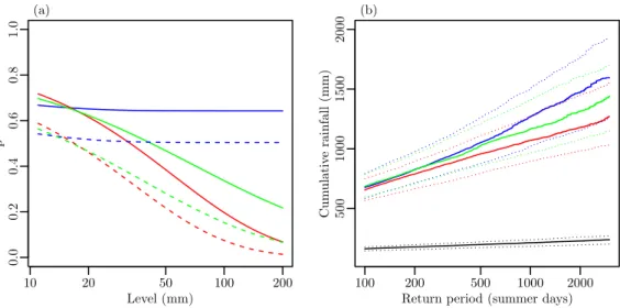
Simulations from our models provide information about quantities depending on the spatial rainfall process, such as return levels for the total amount of rainfall at the 24 sta-tions of the catchment in one day. For a random variable
X of daily records, ther-day return levelxr has probabil-ity Pr(X > xr) = 1/r of being exceeded on one particular day. Return levels for the peaks over threshold model can be derived by inverting (3), and return levels for the total daily rainfall at the 24 stations can be derived by simulation from our model; since we model daily rainfall for summer months, the return levels are expressed in terms of summer days. The estimates shown in Figure 8(b) were obtained by simulating 200,000 summer days and taking empirical quan-tiles of the total amount of rainfall at the 24 stations. The confidence intervals, which are obtained from bootstrapping 200 times using all the summer days of the original data, are rather wide, but the asymptotic independence models give lower estimated return levels. The predictions based on the max-stable model can be seen as giving an upper bound for joint extreme quantities, such as return levels. Figure 8(b) also shows the return levels corresponding to a spatially in-dependent model whose marginal parameters are the same as those estimated for the max-stable Schlather model; this gives much lower return levels and would lead to severe un-derestimation of risk.
6. Discussion
In this paper we propose the use of extreme value mod-els to estimate the extremes of spatial daily rainfall. Our approach consists of fitting generalized Pareto distributions to marginal threshold exceedances and modeling spatial de-pendence using max-stable models or asymptotic indepen-dence models based upon them. For comparison we also con-sider a model based on the Gaussian copula. The models are fitted to threshold exceedances using a censored pair-wise likelihood. Non-stationary models could be fitted by regression on covariates, with model selection performed us-ing CLIC∗. Daily rainfall fields can be simulated over the whole catchment. Estimates of quantities depending on spa-tial extremes, such as joint return levels, can be derived by simulation from the fitted model.
Our application to the Val Ferret watershed, a small mountainous catchment in Swiss Alp, shows that station-ary max-stable and inverted max-stable models seem ap-propriate for modeling extreme rainfall in this small catch-ment. Although max-stable models are natural models for extremes of random fields, model selection seems to favor asymptotic independence models, for which the very rarest events are increasingly local. Simulations from the max-stable model, which assumes stronger dependence, give an upper bound for the effects of joint extremes. Schlather models give simulations that look reasonable, but the Smith model produces unrealistically smooth extremes and is also worst in terms of the information criterion CLIC∗. The Schlather model seems to be appropriate for rainfall in small regions such as Val Ferret, though it cannot model the inde-pendence that would be expected to arise at larger spatial scales. This must be introduced using a Brown–Resnick model or a random set [Davison and Gholamrezaee, 2012]. Indeed, Huser and Davison [2013b] find that a Schlather model with a random set is suitable for a larger hourly sum-mer rainfall dataset, though at a much bigger spatial scale. Rainfall can be simulated over the whole region by apply-ing a marginal transformation to max-stable simulations. In case of spatial non-stationarity, rainfall could be simu-lated by specifying a marginal model for the threshold [as in
Northrop and Jonathan, 2011] and then applying the proce-dure described in §5, with a suitable spatial extrapolation of the empirical distribution functions from observed rainfall sites to ungauged ones. We do not include temporal non-stationarity in our model but with more extensive data this could easily be added.
The interpolation of rainfall values at unobserved sites from nearby observations is generally solved via kriging [ Dig-gle and Ribeiro, 2007], but although this yields “optimal” prediction for Gaussian processes, it may produce unrealis-tic predictions for extremes owing to the unsuitability of a joint Gaussian model. A more appropriate max-stable ap-proach uses conditional simulation of rainfall at ungauged sites [Dombry et al., 2013].
Our approach could be used in other situations where spatial simulation of extreme rainfall is needed. The pro-posed model is appropriate at time-scales for which consec-utive records appear to be independent, which was assumed in our application, but if finer temporal resolution is re-quired, stronger serial correlation will be present and spatio-temporal models will be needed. Max-stable processes have been used for spatio-temporal rainfall byHuser and Davison
[2013b], though fitting and simulating from their model is burdensome.
In many hydrological models for rainfall run-off simula-tion, temperature and other variables that affect predictions from hydrological models are also needed. An open chal-lenge is the joint modeling of these various dependent pro-cesses, taking into account the extremes of some of them.
Acknowledgments. We thank the Swiss National Science Foundation, the ETH Competence Center Environment and Sus-tainability SwissEx and Extremes projects, and Christophe An-cey, Marc Parlange, Simone Padoan and anonymous reviewers for constructive comments. We thank M´et´eoSuisse for making the Grand St-Bernard data available.
References
Banerjee, S., B. Carlin, and A. Gelfand (2004),Hierarchical Mod-eling and Analysis for Spatial Data, Chapman and Hall/CRC, New York.
Beirlant, J., Y. Goegebeur, J. Teugels, and J. Segers (2004), Statistics of Extremes: Theory and Applications, John Wiley, New York.
Blanchet, J., and A. C. Davison (2011), Spatial modelling of ex-treme snow depth,Annals of Applied Statistics,5, 1699–1725, doi:10.1214/11-AOAS464.
Brown, B. M., and S. I. Resnick (1977), Extreme values of inde-pendent stochastic processes,Journal of Applied Probability, 14, 732–739, doi:10.2307/3213346.
Buishand, T. A. (1984), Bivariate extreme-value data and the station-year method, Journal of Hydrology, 69, 77–95, doi: 10.1016/0022-1694(84)90157-4.
Buishand, T. A., L. de Haan, and C. Zhou (2008), On spatial extremes: With application to a rainfall problem, Annals of Applied Statistics,2, 624–642, doi:10.1214/08-AOAS159. Chandler, R. E., V. S. Isham, E. Bellone, C. Yang, and
P. Northrop (2006), Space-Time Modelling of Rainfall for Con-tinuous Simulation, inStatistical Methods for Spatio-Temporal Systems, edited by B. Finkenst¨adt, L. Held, and V. S. Isham, Chapman and Hall/CRC, doi:10.1201/9781420011050.ch5. Chavez-Demoulin, V., and A. C. Davison (2005), Generalized
ad-ditive models for sample extremes,Applied Statistics,54(1), 207–222, doi:10.1111/j.1467-9876.2005.00479.x.
Chavez-Demoulin, V., and A. C. Davison (2012), Modelling time series extremes,Revstat–Statistical Journal,10, 109–133. Coles, S. G. (1993), Regional Modelling of Extreme Storms via
Max-Stable Processes,Journal of the Royal Statistical Society, Series B,55, 797–816.
Coles, S. G. (2001),An Introduction to Statistical Modeling of Extreme Values, Springer-Verlag, London.
Coles, S. G., and J. A. Tawn (1996), Modelling extremes of the areal rainfall process,Journal of the Royal Statistical Society, Series B,58, 329–347.
Cooley, D., D. Nychka, and P. Naveau (2007), Bayesian spa-tial modeling of extreme precipitation return levels, Journal of the American Statistical Association, 102, 824–840, doi: 10.1198/016214506000000780.
Cox, D. R., and V. S. Isham (1988), A simple spatial-temporal model of rainfall,Proceedings of the Royal Society of London, Series A,415, 317–328, doi:10.1098/rspa.1988.0016.
Davis, R. A., and T. Mikosch (2010), The extremogram: A cor-relogram for extreme events, Bernoulli, 15, 977–1009, doi: 10.3150/09-BEJ213.
Davison, A. C., and M. M. Gholamrezaee (2012), Geostatistics of extremes, Proceedings of the Royal Society of London, series A,468, 581–608, doi:10.1098/rspa.2011.0412.
Davison, A. C., and N. I. Ramesh (2000), Local likelihood smoothing of sample extremes,Journal of the Royal Statistical Society, Series B,62, 191–208, doi:10.1111/1467-9868.00228. Davison, A. C., and R. L. Smith (1990), Models for exceedances
over high thresholds (with Discussion),Journal of the Royal Statistical Society, Series B,52, 393–442.
Davison, A. C., S. A. Padoan, and M. Ribatet (2012), Statisti-cal modelling of spatial extremes (with Discussion),Statistical Science,27, 161–186, doi:10.1214/11-STS376.
Davison, A. C., R. Huser, and E. Thibaud (2013), Geostatistics of Dependent and Asymptotically Independent Extremes, Math-ematical Geosciences,45, to appear.
de Carvalho, M., and A. Ramos (2012), Bivariate extreme statis-tics, II,REVSTAT—Statistical Journal,10, 83–107.
de Haan, L. (1984), A spectral representation for max-stable processes, Annals of Probability, 12, 1194–1204, doi: 10.1214/aop/1176993148.
de Haan, L., and A. Ferreira (2006),Extreme Value Theory: An Introduction, Springer, New York.
de Haan, L., and T. T. Pereira (2006), Spatial extremes: Mod-els for the stationary case,Annals of Statistics,34, 146–168, doi:10.1214/009053605000000886.
Diggle, P. J., and P. J. Ribeiro (2007),Model-based Geostatistics, Springer, New York.
Dombry, C., F. ´Eyi-Minko, and M. Ribatet (2013), Conditional simulation of max-stable processes,Biometrika,100(1), 111– 124, doi:10.1093/biomet/ass067.
Feng, S., S. Nadarajah, and Q. Hu (2007), Modeling annual ex-treme precipitation in china using the generalized exex-treme value distribution, Journal of the Meteorological Society of Japan,85, 599–613.
Fisher, R. A., and L. H. C. Tippett (1928), Limiting forms of the frequency distribution of the largest or smallest member of a sample, Mathematical Proceedings of the Cambridge Philosophical Society, 24(02), 180–190, doi: 10.1017/S0305004100015681.
Hall, P., and N. Tajvidi (2000), Nonparametric analy-sis of temporal trend when fitting parametric models to extreme-value data, Statistical Science, 15, 153–167, doi: 10.1214/ss/1009212755.
Huser, R., and A. C. Davison (2013a), Composite likelihood es-timation for the Brown–Resnick process,Biometrika,100, to appear, doi:10.1093/biomet/ass089.
Huser, R., and A. C. Davison (2013b), Space-time modelling of extreme events,Journal of the Royal Statistical Society, series B,75, to appear.
Ingelrest, F., G. Barrenetxea, G. Schaefer, M. Vetterli, O. Couach, and M. Parlange (2010), SensorScope: Application-specific sensor network for environmental monitoring, ACM Trans. Sen. Netw., 6, 17:1–17:32, doi: 10.1145/1689239.1689247.
Kabluchko, Z., M. Schlather, and L. De Haan (2009), Stationary max-stable fields associated to negative definite functions,The Annals of Probability,37, 2042–2065, doi:10.1214/09-AOP455. Katz, R. W., M. B. Parlange, and P. Naveau (2002), Statistics of extremes in hydrology, Advances in Water Resources,25, 1287–1304, doi:10.1016/S0309-1708(02)00056-8.
Langbein, W. B. (1949), Annual floods and the partial-duration flood series, Transactions, American Geophysical Union, 30(6), 879–881.
Ledford, A. W., and J. A. Tawn (1996), Statistics for near in-dependence in multivariate extreme values, Biometrika, 83, 169–187, doi:10.1093/biomet/83.1.169.
Lindsay, B. (1988), Composite likelihood methods,Contemporary Mathematics,80, 221–239.
Madsen, H., P. S. Mikkelsen, D. Rosbjerg, and P. Harremo¨es (2002), Regional estimation of rainfall intensity-duration-frequency curves using generalized least squares regression of partial duration series statistics, Water Resources Research, 38(11), 1239, doi:10.1029/2001WR001125.
Northrop, P. J., and P. Jonathan (2011), Threshold modelling of spatially dependent non-stationary extremes with application to hurricane-induced wave heights (with Discussion), Environ-metrics,22, 799–809, doi:10.1002/env.1106.
Padoan, S. A., M. Ribatet, and S. A. Sisson (2010), Likelihood-based inference for max-stable processes, Journal of the American Statistical Association, 105, 263–277, doi: 10.1198/jasa.2009.tm08577.
Pickands, J. I. (1975), Statistical inference using extreme order statistics, Annals of Statistics, 3, 119–131, doi: 10.1214/aos/1176343003.
R Development Core Team (2012),R: A Language and Environ-ment for Statistical Computing, R Foundation for Statistical Computing, Vienna, Austria, ISBN 3-900051-07-0.
Ramesh, N. I., and A. C. Davison (2002), Local models for ex-ploratory analysis of hydrological extremes,Journal of Hydrol-ogy,256/1–2, 106–119, doi:10.1016/S0022-1694(01)00522-4. Renard, B. (2011), A Bayesian hierarchical approach to regional
frequency analysis, Water Resources Research,47, W11,513, doi:10.1029/2010WR010089.
Ribatet, M. (2011), SpatialExtremes: Modelling Spatial Ex-tremes, R package version 1.8-1.
Rodriguez-Iturbe, I., D. R. Cox, and V. S. Isham (1987), Some models for rainfall based on stochastic point processes, Pro-ceedings of the Royal Society of London, Series A,410, 269– 288, doi:10.1098/rspa.1987.0039.
Rodriguez-Iturbe, I., D. R. Cox, and V. S. Isham (1988), A point process model for rainfall: Further developments,Proceedings of the Royal Society of London, Series A,417, 283–298, doi: 10.1098/rspa.1988.0061.
Salvadori, G., and C. D. Michele (2010), Multivariate multipa-rameter extreme value models and return periods: A cop-ula approach, Water Resources Research, 46, W10,501, doi: 10.1029/2009WR009040.
Sang, H., and A. Gelfand (2010), Continuous Spatial Process Models for Spatial Extreme Values, Journal of Agricultural, Biological, and Environmental Statistics,15(1), 49–65, doi: 10.1007/s13253-009-0010-1.
Schlather, M. (2002), Models for stationary max-stable random fields,Extremes,5(1), 33–44, doi:10.1023/A:1020977924878. Schlather, M., and J. A. Tawn (2003), A Dependence
Measure for Multivariate and Spatial Extreme Values: Properties and Inference, Biometrika, 90, 139–156, doi: 10.1093/biomet/90.1.139.
Shang, H., J. Yan, and X. Zhang (2011), El Ni˜no–Southern Os-cillation influence on winter maximum daily precipitation in California in a spatial model,Water Resources Research,47, W11,507, doi:10.1029/2011WR010415.
Simoni, S., S. Padoan, D. F. Nadeau, M. Diebold, A. Porporato, G. Barrenetxea, F. Ingelrest, M. Vetterli, and M. B. Parlange (2011), Hydrologic response of an alpine watershed: Applica-tion of a meteorological wireless sensor network to understand streamflow generation,Water Resour. Res.,47(10), W10,524, doi:10.1029/2011WR010730.
Smith, R. L. (1990), Max-Stable Processes and Spa-tial Extremes, unpublished manuscript, Univer-sity of Surrey, Guildford GU2 5XH, England. http://www.stat.unc.edu/postscript/rs/spatex.pdf.
Tawn, J. A. (1988), Bivariate extreme value theory: Models and estimation, Biometrika, 75, 397–415, doi: 10.1093/biomet/75.3.397.
Tobin, C., B. Schaefli, L. Nicotina, S. Simoni, G. Barrenetxea, R. Smith, M. Parlange, and A. Rinaldo (2012), Improving the degree-day method for sub-daily melt simulations with physically-based diurnal variations, Advances in Water Re-sources, doi:10.1016/j.advwatres.2012.08.008, in press. Todorovic, P., and J. Rousselle (1971), Some problems of
flood analysis, Water Resour. Res., 7(5), 1144–1150, doi: 10.1029/WR007i005p01144.
Todorovic, P., and E. Zelenhasic (1970), A stochastic model for flood analysis,Water Resour. Res.,6(6), 1641–1648, doi: 10.1029/WR006i006p01641.
Van de Vyver, H. (2012), Spatial regression models for extreme precipitation in Belgium, Water Resources Research, 48(9), W09,549, doi:10.1029/2011WR011707.
Varin, C., and P. Vidoni (2005), A note on composite likelihood inference and model selection, Biometrika, 92(3), 519–528, doi:10.1093/biomet/92.3.519.
Varin, C., N. Reid, and D. Firth (2011), An overview of composite likelihood methods,Statistica Sinica,21, 5–42.
Villarini, G., J. A. Smith, M. L. Baeck, T. Marchok, and G. A. Vecchi (2011), Characterization of rainfall distribu-tion and flooding associated with U.S. landfalling tropical cyclones: Analyses of Hurricanes Frances, Ivan, and Jeanne (2004), Journal of Geophysical Research, 116, D23,116, doi: 10.1029/2011JD016175.
Vrac, M., and P. Naveau (2007), Stochastic downscaling of pre-cipitation: From dry events to heavy rainfalls,Water Resour. Res.,43(7), W07,402, doi:10.1029/2006WR005308.
Wadsworth, J. L., and J. A. Tawn (2012), Dependence mod-elling for spatial extremes, Biometrika,99(2), 253–272, doi: 10.1093/biomet/asr080.
Westra, S., and S. A. Sisson (2011), Detection of non-stationarity in precipitation extremes using a max-stable process model, Journal of Hydrology, 406, 119–128, doi: 10.1016/j.jhydrol.2011.06.014.
Wilks, D. S., and R. L. Wilby (1999), The weather gen-eration game: a review of stochastic weather mod-els, Progress in Physical Geography, 23, 329–357, doi: 10.1177/030913339902300302.
Yang, C., R. E. Chandler, V. S. Isham, and H. S. Wheater (2005), Spatial-temporal rainfall simulation using generalized linear models, Water Resour. Res., 41(11), W11,415, doi: 10.1029/2004WR003739.
Zheng, X., and R. W. Katz (2008), Simulation of spatial depen-dence in daily rainfall using multisite generators, Water Re-sour. Res.,44(9), W09,403, doi:10.1029/2007WR006399.
E. Thibaud, Ecole Polytechnique F´ed´erale de Lausanne, EPFL-FSB-MATHAA-STAT, Station 8, 1015 Lausanne, Switzer-land. ([email protected])
R. Mutzner, School of Architecture, Civil and Environmental Engineering, Ecole Polytechnique F´ed´erale de Lausanne, Station 2, 1015 Lausanne, Switzerland. ([email protected])
A. C. Davison, Ecole Polytechnique F´ed´erale de Lausanne, EPFL-FSB-MATHAA-STAT, Station 8, 1015 Lausanne, Switzer-land. ([email protected])
Figure 1. The Val Ferret watershed, showing the sites of the meteorological stations, with contours showing their elevations above mean sea level in meters.
0 100 300 500 0 20 40 60 1 Time mm 0 100 300 500 0 20 40 60 2 Time mm 0 100 300 500 0 20 40 60 3 Time mm 0 100 300 500 0 20 40 60 4 Time mm
Figure 2. Daily cumulative rainfall totals for 575 days in summers 2009 to 2012, recorded by Sensorscope stations 1–4 in the Val Ferret region. Vertical dashed lines sepa-rate the four years. White spaces correspond to missing data. 0 20 60 100 Time mm 1982 1987 1992 1997 2002 2007 2012
Figure 3. Daily cumulative rainfall totals for 31 years in summers 1982 to 2012, recorded by M´et´eoSuisse at the Grand St-Bernard.
0 10 20 30 40 50 0.00 0.15 0.30 1 Lag 0 10 20 30 40 50 0.00 0.15 0.30 2 Lag 0 10 20 30 40 50 0.00 0.15 0.30 3 Lag 0 10 20 30 40 50 0.00 0.15 0.30 4 Lag
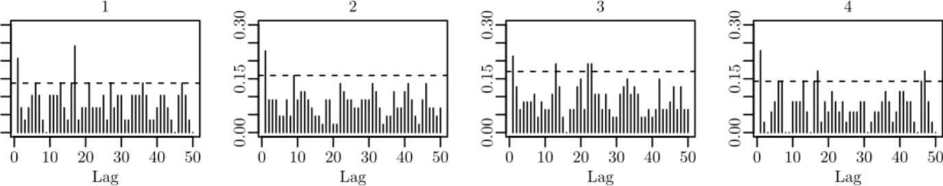
Figure 4. Extremogram (4) for the daily cumula-tive rainfall time series at four locations computed with thresholds corresponding to the 90% quantile for each se-ries. Horizontal dashed lines show the upper 0.975 con-fidence limit for independent data, obtained by random permutation of the data.
10 20 50 100 500 2000 10 20 50 100 200 500 1000 Theoretical Quantiles Sample Quan tiles
Figure 5. Pooled unit Fr´echet QQ-plot for the marginal fits of model (12) with the Schlather model. The same marginal model is fitted to the data from all the 24 locations in the catchment. Dotted lines are the 95% confidence bounds, obtained by simulating from fitted model (12). The solid diagonal line indicates a perfect fit. 572 573 574 575 576 577 79 80 81 82 83 84 85 (a) 572 573 574 575 576 577 79 80 81 82 83 84 85 (b) 572 573 574 575 576 577 79 80 81 82 83 84 85 (c) 0 10 20 30 40 50
Figure 6. Simulation of max-stable random fields, on the original data scale (mm), from the fitted (a) Smith and (b) Schlather models and (c) an inverted max-stable process based on the Schlather model. Black dots show the locations of the 24 stations. Distances (km) have as origin the Swiss coordinate system (CH1903) and the contour shows the Val Ferret watershed, as in Figure 1.
0 1 2 3 4 5 6 1.0 1.2 1.4 1.6 1.8 2.0 Distance (km) θ
(
h)
(a) 0 1 2 3 4 5 6 7 0.5 0.6 0.7 0.8 0.9 1.0 Distance (km) η(
h)
(b)Figure 7. Fitted extremal coefficients (a) and tail de-pendence coefficients (b) for the different models. In (a), the hatched polygon shows the limits of the Smith ex-tremal coefficient curves, which are direction-dependent. In (b), the solid line corresponds to the Gaussian cop-ula model. In both plots, dashed lines correspond to the Schlather model and dotted lines to the Brown–Resnick model. Points are the estimated coefficients for pairs of stations grouped into distance classes, with 95% con-fidence intervals, obtained by bootstrapping the daily data, shown as grey vertical lines.
10 20 50 100 200 0.0 0.2 0.4 0.6 0.8 1.0 Level (mm) p (a) 100 200 500 1000 2000 500 1000 1500 2000
Return period (summer days)
Cum
ulativ
e rainfall (mm)
(b)
Figure 8. Comparison of results from max-stable and asymptotic independence models. Panel (a): the-oretical conditional probabilities of exceedances p(y) = Pr{Y(x1)> y|Y(x2)> y}for pairs of locations{x1, x2} 1 km apart (plain lines) and 5 km apart (dashed lines). Panel (b): return levels (solid) with 95% confidence in-tervals (dotted), for the total daily rainfall falling at the 24 stations in the Val Ferret watershed. In both panels, blue lines correspond to the Schlather max-stable model, red lines to the inverted max-stable Schlather model and green lines to the Gaussian copula model. Black lines in (b) correspond to a spatially independent model.