ISSN 1450-2887 Issue 22 (2010) © EuroJournals, Inc. 2010 http://www.eurojournals.com
Testing World Consumption Asset Pricing Models
Bin Li
Griffith Business School, Griffith University, Brisbane, QLD 4111, Australia
E-mail: [email protected] Tel: +61-7- 3735 7117
Abstract
Using data for 17 countries, this study empirically examine the performance of four consumption-based capital asset pricing models (CCAPM): the classic world CCAPM under the assumption of complete international markets integration, the heterogeneous world CCAPM under the framework of Constantinides and Duffie (1996) and two world habit models. The nonlinear models are estimated and tested by Hansen’s (1982) GMM. The empirical results suggest that a large and economically implausible coefficient of relative risk aversion is needed to resolve the equity premium puzzle for the classic world CCAPM; by contrast, more sophisticated consumption models (the heterogeneous world CCAPM and the world surplus CCAPM) are able to generate an equity premium at lower coefficients of relative risk aversion. The study provides another piece of evidence supporting consumption-based models, particularly the heterogeneous world CCAPM and the world surplus CCAPM, for asset pricing in international markets.
Keywords: CCAPM, Consumption Model, International Financial Markets, Heterogeneous Consumption, Habit Formation
JEL Classification Codes: G12, G15
1. Introduction
The consumption-based capital asset pricing model (CCAPM) is the simplest and most intuitive of all asset-pricing models (Cochrane, 2001). Developed by Lucas (1978), Breeden (1979) and others, the CCAPM follows from the first-order condition for a utility-maximising agent’s intertemporal consumption and investment choice problem. In equilibrium, the agent invests to the point where the marginal utility lost from foregoing current consumption is equal to the discounted expected marginal utility gained from that investment in the future.
Most tests of the CCAPM are often performed in a domestic setting, although theory suggests that the CCAPM is equally applicable across countries. Researchers often assume that there are three types of market linkage in the international finance literature (Bekaert and Harvey, 1995): complete integration, complete segmentation, and mild segmentation. In a completely integrated market, asset prices are determined by a world stochastic discount factor (SDF), which implies that the SDFs for asset returns in each country should be related to aggregate world variables rather than country-specific variables. Under the assumption of complete segmentation, asset pricing models are tested using domestic data only. Under the hypothesis of mild segmentation, asset returns are not only related to domestic factors but also to world factors.
The world CAPM, in which the excess return on the world market is a factor, is typically tested in empirical research on international asset pricing (e.g., Stehle, 1997; Korajczyk and Viallet, 1989; Harvey, 1991; Chan, Karolyis and Stulz, 1992; and De Santis and Gerard, 1997). Researchers also consider factors from other models. E.g., Cho, Eun and Senbet (1986) consider factors from the international arbitrage pricing theory; Ferson and Harvey (1993) consider global economic factors; Jorion (1991), Dumas and Solnik (1995), and De Santis and Gerard (1998) consider exchange rate risk.
The consumption-based asset pricing model would be preferred over the world CAPM where differences in consumption baskets across markets are an important factor in determining the cross-sectional variation in stock returns (Karolyi and Stulz, 2003). However, research on the consumption CAPM in the international setting is still quite limited. Wheatley (1988) uses the CCAPM to test international equity market integration. Cumby (1990) tests a consumption-based international asset pricing model using the MSCI market indices data for the US, the UK, Germany and Japan. Li and Zhong (2005) apply habit-formation models to investigate the predictability and cross-sectional returns from international equity markets. They find that the surplus consumption associated with a common world SDF can partly explain the returns on most developed equity markets and the habit CCAPM performs well in cross-sectional tests. Sarkissian (2003) studies the CCAPM in foreign exchange markets under the assumption of imperfect risk sharing across countries and he finds that the new CCAPM with the cross-country consumption dispersion as a factor can better explain the currency risk premium than the classic CCAPM. Li and Zhong (2009) incorporate both habit formation and uninsurable idiosyncratic risks into an international CCAPM and they find that the model can explain a large fraction of the variation in the cross section of currency and equity premiums in developed countries.
In this paper, I study the empirical performance of various consumption models for international equity markets. I use data for 17 MSCI countries to examine whether consumption variables are related to excess returns on the market indices in different countries. The study contributes to the literature by providing empirical analysis of the incomplete risk sharing in the explanation of the international stock returns.
I start with the classic world CCAPM under the assumption of complete market integration and complete risk sharing. Under the assumption that a representative investor has a power utility, world consumption growth is the only factor that determines asset returns in the classic world CCAPM. However, when there is imperfect consumption risk sharing across countries, investors can face persistent consumption shocks and consequently the cross-sectional variance of consumption growth can affect asset pricing (Constantinides and Duffie, 1996). Thus in the heterogeneous CCAPM, asset returns are not only related to world consumption growth, but also related to the cross-country variation in consumption growth. Sarkissian (2003) uses the heterogeneous CCAPM to study international currency premiums. As the heterogeneous CCAPM can also be applied to equity markets, I investigate whether this model has explanatory power for the return variation on international equity markets. Moreover, I extend the Abel (1990) and Campbell and Cochrane (1999) habit models to the international setting to investigate whether the more sophisticated consumption models have better performance.
Using Hansen’s (1982) generalized method of moment (GMM), I find that an economically implausibly large risk aversion is needed to address the equity premium for the classic world CCAPM. By contrast, with an additional factor (a cross-country consumption dispersion factor), the heterogeneous world CCAPM has significantly lower and economically more plausible coefficient estimates of consumption risk aversion.
The empirical findings of this study provide new evidence for the international asset pricing using consumption models. The more sophisticated consumption models are preferred over the classic CCAPM to reduce the extent of the equity premium puzzle as they are able to generate equity premiums at lower coefficients of risk aversion. The findings highlight the importance of cross-country consumption dispersion as well as world consumption growth in determining the expected excess returns on stock markets.
The remainder of this paper is organised as follows. Section 2 introduces different world consumption models. It starts with the classic world CCAPM and then extends to the heterogeneous world CCAPM. For comparison, I also present the world surplus consumption model and Abel’s habit model. Section 3 describes the data and discusses the variables used in asset pricing models. It also provides summary statistics. Section 4 presents econometric method and the empirical results from GMM estimation. Section 5 concludes.
2. World Consumption CAPM
In this section, I describe the models employed in the empirical testing. I first introduce the classic world CCAPM in which there is a representative agent in the complete world market. Then I describe the heterogeneous world CCAPM under the Constantinides and Duffie (1996) framework in which there is incomplete consumption risk sharing in the market and therefore the variation in idiosyncratic consumption growth should be priced. For comparison, I also present two habit models in the international setting: the Campbell and Cochrane (1999) surplus consumption model and the Abel (1990) ratio habit model.
2.1. Classic World CCAPM
Stulz (1981a, b) notes that asset prices from all countries are determined by a common stochastic discount factor under the assumption of complete international market integration and complete consumption risk sharing. In terms of the consumption-based asset pricing model, the expected returns of the assets the representative investor holds in the world market are determined by their covariance with the per capita aggregate world consumption growth. With the assumption of the power utility function, the representative investor maximises his life-time utility
1 0 , 1 w t t t w t w C E γ
δ
γ
− ∞ = −∑
(1)where Ct is the real per capita world consumption, δwt is the subjective time discount factor, and w
γ
is the utility curvature parameter, also called the coefficient of relative risk aversion of the world representative investor. The Euler equation for the investor’s optimisation problem is, 1 , 1 0, e t w t i t E M⎡⎣ +R + ⎤ =⎦ (2) where e, 1 i t
R + is the excess return on the asset in country i from date t to t+1, and , 1 , 1 , w w t w t w t C M C γ − + + ⎛ ⎞ = ⎜⎜ ⎟⎟ ⎝ ⎠ is his stochastic discount factor. (2) is the SDF representation of the classic world CCAPM.
2.2. Heterogeneous World CCAPM
The classic world CCAPM is based on the complete market assumption. Constantinides and Duffie (1996, hereafter CD) introduce heterogeneity effects into the CCAPM framework. CD assume an economy where an individual investor k has his own consumption level Ck t, , but all investors have the same power utility function with the same time discount factor δ, and coefficient of relative risk aversion
γ
. Under the assumption of the existence of permanent income shocks, they derive the Euler equation for the heterogeneous CCAPM, which is, 1 2 1 , 1 , ( 1) e x p 0 , 2 k t e t t k t k t C E d R C γ γ γ δ − + + + ⎡ ⎛ ⎞ ⎛ + ⎞ ⎤ ⎢ ⎜⎜ ⎟⎟ ⎜ ⎟ ⎥ = ⎢ ⎝ ⎠ ⎝ ⎠ ⎥ ⎣ ⎦ (3) where dt+1is the cross-sectional standard deviation of consumption growth (or labelled as
the cross-sectional consumption dispersion on the currency risk premium in foreign exchange markets. I follow Sarkissan’s approach but instead I examine the heterogeneous world CCAPM in equity markets.
In the international setting, the Euler equation can be rewritten as
, 1 * , 1 , 1 , ( 1) exp 0, 2 j t e t j t j t j t C E d R C γ γ γ δ − + + + ⎡ ⎛ ⎞ ⎛ + ⎞ ⎤ ⎢ ⎜⎜ ⎟⎟ ⎜ ⎟ ⎥ = ⎢ ⎝ ⎠ ⎝ ⎠ ⎥ ⎣ ⎦ (4)
where Cj t, is the aggregate consumption in country k at date t, *
(
)
, 1 var ln , 1/ ,j t k kj t kj t
d + = ⎡⎣ C + C ⎤⎦ is the cross-sectional variance of log consumption growth in country j, and Ckj t, is the consumption of investor k in country j.
Assuming there are consumption heterogeneities both within and across countries, Sarkissan develops an Euler equation for country j:
(
)
, 1 * 1 , 1 , 1 , ( 1) exp 0, 2 w t w e t t j t j t w t C E d d R C γ γ γ δ − + + + + ⎡ ⎛ ⎞ ⎛ + ⎞ ⎤ ⎢ ⎜⎜ ⎟⎟ ⎜ + ⎟ ⎥= ⎢ ⎝ ⎠ ⎝ ⎠ ⎥ ⎣ ⎦ (5) where w1 var ln(
, 1/ ,)
t j j t j td+ = ⎡⎣ C + C ⎤⎦is the cross-country variance of consumption growth. According to
the heterogeneous CCAPM in (5), asset returns are related to world consumption growth, and the within- and cross-country variance of consumption growth. Since it is difficult to obtain data to construct the within-country variance of consumption growth, I follow Sarkissan to assume
*
, 1 ( 1) 1 w
j t t
d + = η− d+ , where
η
is a scale factor representing cross-sectional consumption variation above and beyond cross-country dispersion. Then (5) can be rewritten as, 1 1 , 1 , ( 1) exp 0, 2 w t w e t t j t w t C E d R C γ γ γ δ η − + + + ⎡ ⎛ ⎞ ⎛ + ⎞ ⎤ ⎢ ⎜⎜ ⎟⎟ ⎜ ⎟ ⎥ = ⎢ ⎝ ⎠ ⎝ ⎠ ⎥ ⎣ ⎦ (6)
and the SDF of the heterogeneous world CCAPM is , 1
1 1 , ( 1) exp 2 w t w t t w t C M d C γ γ γ δ η − + + + ⎛ ⎞ ⎛ + ⎞ = ⎜⎜ ⎟⎟ ⎜ ⎟ ⎝ ⎠ ⎝ ⎠ .
2.3. World Surplus CCAPM
Campbell and Cochrane (1999) propose a habit model where the investor’s utility is a function of the difference between consumption and habit, and the SDF of this model depends upon the surplus consumption ratio. Hence, I call this model the surplus consumption model. Accordingly, the model extended to the international setting under the assumption of complete markets is called the world surplus consumption model. The SDF of the world surplus CCAPM is
, 1 , 1 1 , , , w w t w t t w t w t S C M S C γ δ − + + + ⎛ ⎞ = ⎜⎜ ⎟⎟ ⎝ ⎠ (7) where Sw t, is the world surplus consumption ratio.
2.4. Abel’s (1990) Habit World CCAPM
Abel (1990) models current-period utility as a function of current-period consumption, assessed relative to the prior-period consumption. Specifically, the relativities of current-to-prior consumption take a ratio form. In the framework of the world CCAPM, the world representative investor solves the following optimisation problem:
(
)
1 , , 1 1 max 1 w t v w t v v t v C X E γ δ γ − ∞ + + = ⎡ − ⎤ ⎢ ⎥ − ⎢ ⎥ ⎣∑
⎦ (8)where Xw,t captures the impact of past consumption on current utility. Abel (1990) adopts Xw t, Cw t, 1
κ −
= , such that habit depends on just one lag of consumption and the parameter κ reflects the degree of time nonseparability. Under Abel’s (1990) model, the first-order condition is
( 1) , 1 , , 1 , , 1 0 w t w t e t j t w t w t C C E R C C γ κ γ δ − − + + − ⎡ ⎛ ⎞ ⎛ ⎞ ⎤ ⎢ ⎜⎜ ⎟ ⎜⎟ ⎜ ⎟⎟ ⎥ = ⎢ ⎝ ⎠ ⎝ ⎠ ⎥ ⎣ ⎦ . (9)
3. Data and Summary Statistics
3.1. Main VariablesThe test assets in this study are the Morgan Stanley Capital International (MSCI) stock market indices from 17 countries which are sourced from DataStream: Australia, Austria, Belgium, Canada, Denmark, France, Germany, Hong Kong, Italy, Japan, Netherlands, Norway, Spain, Sweden, Switzerland, the UK, and the US. These indices are value-weighted and adjusted for dividend reinvestment. Following Harvey (1991) and Li and Zhong (2005), I calculate excess returns on the indices as the returns on the MSCI country indices in US dollars less the returns on the risk-free asset, which is proxied by the three-month US Treasury bill rate. The US Treasury bill rate is obtained from the international financial statistics (IFS). I obtain monthly MSCI price indices and Treasury bill rate to calculate quarterly returns. As the monthly price indices are reported using the prices at the beginning of each month, the quarterly return is calculated as the log of the price at the first month in the following quarter divided by the price at the first month in this quarter.1 The quarterly sample period starts from 1970Q2 through 2007Q4.
My testing of the world CCAPM requires a world consumption index, which can be constructed from local consumption data. As there is no consumption data available for some countries (Belgium, Denmark, HK, and Norway) in the early period of the sample, I use the consumption data from the remaining countries to construct the world consumption index. Though the theory of the CCAPM requires the use of household non-durables and services consumption, these data are not available for most countries. Therefore, I use household or private total consumption in each country instead. The real per-capita consumption for each 13 countries is constructed as local consumption in local currency divided by local consumer price index (CPI) and local population. The consumption, population and CPI data are sourced from DataStream, and their original source is the IFS.2 The consumption data are seasonally adjusted except for Austria, Norway, and Sweden. I use the X11 procedure in the RATS software to convert these non-seasonally adjusted data into seasonally-adjusted units. As the population data is in annual terms for each country, I use the interpolation procedure in
1 For example, the return on the first quarter of 1980 is calculated as
1980 1Q ln( 1980M4/ 1980M1)
r = P P
,
where P1980M4 and P1980M1 are the prices in April and January respectively. The return on the US Treasury bill rate in 1980Q1 is calculated as
(
)
,1980 1 ln (1 ,1980 1)*(1 ,1980 2)*(1 ,1980 3) f Q f M f M f M r = +r +r +r , and then the excess return in 1980Q1 is calculated as1980Q1 1980 1 ,1980 1 e
Q f Q
r =r −r
2 As consumption data for Canada, Japan, and the US are in annual amount from DataStream, I convert them to the
RATS to interpolate them into quarterly numbers.3 I also convert the non-seasonally adjusted CPI data to seasonally adjusted numbers. The real per-capita consumption growth in each country is constructed as 1 ln( / ) t t t c C C− Δ = . (10)
I follow Sarkissan (2003), and Li and Zhong (2005) to construct a world consumption index from the gross domestic product (GDP) weighted average of local real per-capita consumption growth. The quarterly growth rate of the world consumption index is a weighted average of the real consumption growth in each country with its GDP weighting in the world GDP, which is the sum of the GDPs of the 13 countries. The weighting for each quarter is determined by the GDP in US dollars at the beginning of the quarter. The quarterly GDP data are obtained from DataStream and their original source is the IFS. 4 I also use the X11 procedure to convert the non-seasonally adjusted GDP data for Austria, Norway, and Sweden into seasonally-adjusted units. As the GDP data are in local currency, I obtain the foreign exchange data from DataStream to convert them into dollar terms. I obtain MSCI FC/US$ for Australian Dollar, Canadian Dollar, Hong Kong Dollar, Norwegian Krona, Swedish Krona, and Swiss Franc, and UK Sterling. The exchange rates for other currencies are quoted in terms of UK Sterling from the world market. Then the cross rate for other currencies against US$ can be derived as the multiplication of the FC/UK£ and UK£/US$.
3.2. Instrumental Variables
The instrumental variables in the GMM tests include the lagged world consumption growth, the lagged US consumption-wealth ratio, and the lagged US term spread. The US consumption-wealth ratio is from the website of Martin Lettau which is constructed as per Lettau and Ludvigson (2001a, 2001b). The US term spread is the 10-year US government bond yield minus the US 3-month Treasury bill rate. The choice of the instruments is based on previous studies (e.g., Harvey, 1991; Bekaert and Harvey, 1995; and Li and Zhong, 2005).
3.3. Summary Statistics
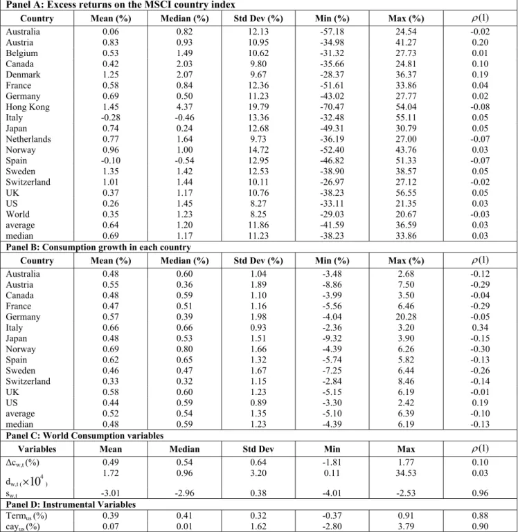
Table 1 reports summary statistics for the 17 countries. Mean, median, standard deviation, and minimum, maximum and the first-order autocorrelation coefficients are reported. The sample period starts from 1970Q2 through 2007Q4 (151 observations). Panel A reports summary statistics of the quarterly excess return on the MSCI country indices. The excess returns are calculated in US dollars in excess of the holding period return on the three-month US Treasury bill. The 17 countries are: Australia, Austria, Belgium, Canada, Denmark,
3 Li and Zhong (2005) also interpolate the population data.
4 As GDP data for Canada, Japan, and the US are in annual amount from DataStream, I convert them to the quarterly
Table 1: Summary Statistics
Panel A: Excess returns on the MSCI country index
Country Mean (%) Median (%) Std Dev (%) Min (%) Max (%) ρ(1)
Australia 0.06 0.82 12.13 -57.18 24.54 -0.02 Austria 0.83 0.93 10.95 -34.98 41.27 0.20 Belgium 0.53 1.49 10.62 -31.32 27.73 0.01 Canada 0.42 2.03 9.80 -35.66 24.81 0.10 Denmark 1.25 2.07 9.67 -28.37 36.37 0.19 France 0.58 0.84 12.36 -51.61 33.86 0.04 Germany 0.69 0.50 11.23 -43.02 27.77 0.02 Hong Kong 1.45 4.37 19.79 -70.47 54.04 -0.08 Italy -0.28 -0.46 13.36 -32.48 55.11 0.05 Japan 0.74 0.24 12.68 -49.31 30.79 0.05 Netherlands 0.77 1.64 9.73 -36.19 27.00 -0.07 Norway 0.96 1.00 14.72 -52.40 43.76 0.03 Spain -0.10 -0.54 12.95 -46.82 51.33 -0.07 Sweden 1.35 1.42 12.53 -38.90 38.57 0.05 Switzerland 1.01 1.44 10.11 -26.97 27.12 -0.02 UK 0.37 1.17 10.76 -38.23 56.55 0.05 US 0.26 1.45 8.27 -33.11 21.35 0.03 World 0.35 1.23 8.25 -29.03 20.67 -0.03 average 0.64 1.20 11.86 -41.59 36.59 0.03 median 0.69 1.17 11.23 -38.23 33.86 0.03
Panel B: Consumption growth in each country
Country Mean (%) Median (%) Std Dev (%) Min (%) Max (%) ρ(1)
Australia 0.48 0.60 1.04 -3.48 2.68 -0.12 Austria 0.55 0.36 1.89 -8.86 7.50 -0.29 Canada 0.48 0.59 1.10 -3.99 3.50 -0.04 France 0.47 0.51 1.16 -5.56 6.46 -0.29 Germany 0.57 0.39 1.98 -4.04 20.28 -0.05 Italy 0.66 0.66 0.93 -2.36 3.20 0.34 Japan 0.48 0.53 1.51 -9.32 3.90 -0.15 Norway 0.69 0.80 1.66 -4.39 6.26 -0.30 Spain 0.62 0.65 1.32 -5.74 5.82 -0.13 Sweden 0.46 0.47 1.67 -7.25 6.44 -0.26 Switzerland 0.33 0.32 1.15 -2.84 8.46 -0.14 UK 0.58 0.60 1.23 -5.15 6.19 -0.01 US 0.44 0.59 0.89 -3.30 2.42 0.19 average 0.52 0.54 1.35 -5.10 6.39 -0.10 median 0.48 0.59 1.23 -4.39 6.19 -0.13
Panel C: World Consumption variables
Variables Mean Median Std Dev Min Max ρ(1)
Δcw,t (%) 0.49 0.54 0.64 -1.81 1.77 0.10 dw,t ( 4 10 × ) 1.72 0.96 3.20 0.11 34.53 0.03 sw,t -3.01 -2.96 0.38 -4.01 -2.53 0.96
Panel D: Instrumental Variables
Termus (%) 0.39 0.41 0.32 -0.37 0.91 0.88
cayus (%) 0.07 0.01 1.62 -2.80 3.79 0.90
Notes: This table reports mean, median, standard deviation, and minimum, maximum and the first-order autocorrelation coefficients of the variables. The sample period starts from 1970Q2 through 2007Q4.
Panel A reports summary statistics of the quarterly excess return on the MSCI country indices. The excess returns are calculated in US dollars in excess of the holding period return on the three-month US Treasury bill. There are 17 countries: Australia, Austria, Belgium, Canada, Denmark, France, Germany, Hong Kong, Italy, Japan, Netherlands, Norway, Spain, Sweden, Switzerland, the UK, and the US. The numbers are in percentage except for ρ(1).
Panel B: reports summary statistics of the real per capita consumption growth in 13 countries.
Panel C: reports summary statistics of world consumption growth Δcw,t, the cross-sectional dispersion of consumption growth dw,t, and the log world surplus consumption ratio sw,t. Except for ρ(1), the numbers for the world consumption growth is in percentage and for the cross-sectional dispersion of consumption growth is multiplied by 104.
Panel D: reports summary statistics of instrumental variables: the US term spread Termus and the US consumption-wealth ratio cayus. The numbers are in percentage except for ρ(1).
Germany, Hong Kong, Italy, Japan, Netherlands, Norway, Spain, Sweden, Switzerland, the UK, and the US. The highest mean excess return over the sample is 1.45% per quarter from the Hong Kong market. Hong Kong also has the highest standard deviation. The mean excess returns for the US market is lower than most other markets, and the US has the lowest standard deviation. These findings are consistent with Harvey (1991) whose sample period is the early part of my sample period. The returns on the Italian and Spanish markets are negative, which suggests the returns on the market indices in US dollars in these two countries are less than the return on the US Treasury bill on average. As the MSCI world market portfolio is a value-weighted average of country returns, it achieves a lower standard deviation than any of the 17 markets due to market diversification. The first-order autocorrelation coefficient is low for each country.
Panel B reports summary statistics of the real per capita consumption growth in 13 countries. The time-series average of consumption growth does not differ much across countries. The first-order coefficients are all negative except for Italy and the US, suggesting that there is mean-reversion in consumption growth in most countries.
Panel C shows summary statistics for the main variables used in asset pricing tests. These variables are the world consumption growth, the cross-sectional consumption dispersion, and the world surplus consumption ratio. It shows that the mean world consumption growth rate is 0.49%, which is close to the consumption growth in the US. The standard deviation for the world consumption growth is 0.64%, which is lower than the corresponding figure for the US. The range between the minimum and the maximum for the world consumption growth is smaller than the one for the US. This is because the world consumption growth is constructed as a GDP-weighted average of consumption growth in 13 countries, and consequently the series become smoother. The cross-sectional dispersion of consumption growth has a mean of 0.0172%, and the first-order autocorrelation is only 0.03. Compared to the world consumption growth and the cross-sectional consumption dispersion, the world surplus consumption ratio has a low standard deviation and a high autocorrelation.
Panel D shows summary statistics of instrumental variables: the US term spread and the US consumption-wealth ratio. The first-order autocorrelations for these two variables are close to 0.90.
4. Econometric Method and Empirical Results
4.1. Econometric Method
In this section, I estimate the coefficients of relative risk aversion γ and test the four consumption models: the world CCAPM, the heterogeneous world CCAPM, the world surplus CCAPM, and the Abel habit model. I first examine these models for all the G7 countries (Canada, France, Germany, Italy, Japan, the UK, and the US) and the world market simultaneously. Then all markets in 17 countries are considered at the same time.
Hansen’s (1982) GMM methodology is employed to estimate and test the models. Following Sarkissan (2003), I model the mean pricing errors for each asset as the parameters to be estimated along with γ.5 The error term for the heterogeneous world CCAPM is defined as6
, 1 , 1 1 , 1 , ( 1) exp ( ), 2 w t w e j t t j t j w t C u d R C γ γ γ η α − + + + + ⎛ ⎞ ⎛ + ⎞ =⎜⎜ ⎟⎟ ⎜ ⎟ − ⎝ ⎠ ⎝ ⎠ (11) where α j is the mean pricing error for asset j, which is the difference between the realised excess
return on asset j and the fitted return predicted by the asset pricing model. If we set η to zero, (11) collapses to the error term for the classic world CCAPM. The moment restrictions for GMM estimation are7
5 The advantage of this approach is that it enables us to compare pricing errors across different models.
6 As my focus is on the estimations of the coefficients of relative risk aversion, I omit the time discount factor δ (assuming
δ=1) in error terms.
1( , 1 ) 0, 1, , e t j t j t E M⎣⎡ + R + −α z ⎤⎦= i= … N (12) where , 1 1 1 , ( 1) exp 2 w t w t t w t C M d C γ γ γ η − + + + ⎛ ⎞ ⎛ + ⎞ = ⎜⎜ ⎟⎟ ⎜ ⎟ ⎝ ⎠ ⎝ ⎠
, and zt is an I×1vector of instrumental variables known at time t. (12) represents N×I moment restrictions implied by the Euler equations for N asset returns. There are N+1 parameters, γ and αj(j=1, , )… N to be estimated. Therefore the Hansen J-test has (N×I-N-1) overidentifying restrictions. The moment restrictions for the world surplus consumption model and the Abel habit model can be derived accordingly.
I use two-step GMM to estimate the models with the identity weighting matrix in the first stage. I use the Newey and West (1987) heteroskedasticity and autocorrelation (HAC) consistent matrix with two lags length to obtain t-statistics for the estimates.
For model comparison, I use the mean pricing errors generated by each model. I also report the Hansen and Jagannathan (1997) distance to compare each model’s performance. Hansen and Jagannathan (1997) develop a measure of how badly a general asset pricing model is misspecified using an estimate of its SDF. It can assess the relative fit of nonnested models. Hansen and Jagannathan look at the shortest distance between the estimated SDF, *
1 t
M+ , and the true SDF Mt+1,
* 1 1 min t t HJD= M+ −M+ , such that 1 e1 0 t t E M R⎡⎣ + + ⎤ =⎦ . (13) They show that HJD can be expressed as
1/ 2 1 * ' * 1 1 1 1 1 1 , e e e e t t t t t t HJD= ⎜⎛E M R⎣⎡ + + ⎦ ⎣⎤ ⎡′E R R+ + ⎤⎦− E M R⎡⎣ + + ⎤⎦⎞⎟ ⎝ ⎠ (14)
and HJD can be interpreted as the maximum pricing error among the set of assets. Then the lowest HJD implies that the corresponding SDF is closer to the true SDF.
4.2. Empirical Results
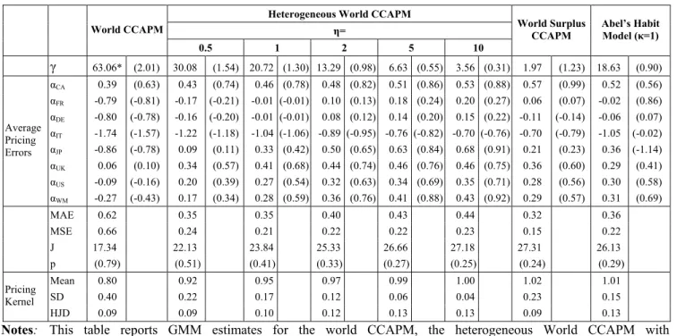
Table 2 reports the GMM estimates for the world CCAPM, the heterogeneous World CCAPM with the parameter η being set to 0.5, 1, 2, 5, 10, respectively, the world surplus CCAPM, and the Abel habit model with the parameter κ set to1. The test assets are the MSCI country indices in the G7 countries (Canada, France, Germany, Italy, Japan, the UK, and the US) plus the world market index. GMM systems use all the test assets simultaneously. The instruments include a constant, the lagged values of the world consumption growth, the US term spread and the US consumption-wealth ratio. The table reports the estimated coefficient of risk aversion γ, average pricing error for each market α, and the corresponding t-statistic is given in parentheses. I also report the mean absolute pricing errors (MAE) and mean squared pricing errors (MSE) for each model, the means and standard deviations (SD) of the estimated SDFs, and the Hansen J-test and its associated p-value in parentheses on the next right column. The last row reports the Hansen and Jagannathan (1997) distance (HJD) of the estimated SDFs. My sample starts from 1970Q3 through 2007Q3 (149 observations).
Table 2: Tests of the Euler Equations (G7+World)
Heterogeneous World CCAPM
η= World CCAPM 0.5 1 2 5 10 World Surplus CCAPM Abel’s Habit Model (κ=1) γ 63.06* (2.01) 30.08 (1.54) 20.72 (1.30) 13.29 (0.98) 6.63 (0.55) 3.56 (0.31) 1.97 (1.23) 18.63 (0.90) αCA 0.39 (0.63) 0.43 (0.74) 0.46 (0.78) 0.48 (0.82) 0.51 (0.86) 0.53 (0.88) 0.57 (0.99) 0.52 (0.56) αFR -0.79 (-0.81) -0.17 (-0.21) -0.01 (-0.01) 0.10 (0.13) 0.18 (0.24) 0.20 (0.27) 0.06 (0.07) -0.02 (0.86) αDE -0.80 (-0.78) -0.16 (-0.20) -0.01 (-0.01) 0.08 (0.12) 0.14 (0.20) 0.15 (0.22) -0.11 (-0.14) -0.06 (0.07) αIT -1.74 (-1.57) -1.22 (-1.18) -1.04 (-1.06) -0.89 (-0.95) -0.76 (-0.82) -0.70 (-0.76) -0.70 (-0.79) -1.05 (-0.02) αJP -0.86 (-0.78) 0.09 (0.11) 0.33 (0.42) 0.50 (0.65) 0.63 (0.84) 0.68 (0.91) 0.21 (0.23) 0.36 (-1.14) αUK 0.06 (0.10) 0.34 (0.57) 0.41 (0.68) 0.44 (0.74) 0.46 (0.76) 0.46 (0.75) 0.36 (0.60) 0.29 (0.41) αUS -0.09 (-0.16) 0.20 (0.39) 0.27 (0.54) 0.32 (0.63) 0.34 (0.69) 0.35 (0.71) 0.28 (0.56) 0.30 (0.58) Average Pricing Errors αWM -0.27 (-0.43) 0.17 (0.34) 0.28 (0.59) 0.36 (0.76) 0.41 (0.88) 0.43 (0.92) 0.29 (0.57) 0.31 (0.69) MAE 0.62 0.35 0.35 0.40 0.43 0.44 0.32 0.36 MSE 0.66 0.24 0.21 0.22 0.22 0.23 0.15 0.22 J 17.34 22.13 23.84 25.33 26.66 27.18 27.31 26.13 p (0.79) (0.51) (0.41) (0.33) (0.27) (0.25) (0.24) (0.29) Mean 0.80 0.92 0.95 0.97 0.99 1.00 1.02 1.01 SD 0.40 0.22 0.17 0.12 0.06 0.04 0.23 0.15 Pricing Kernel HJD 0.09 0.09 0.10 0.12 0.13 0.13 0.09 0.13
Notes: This table reports GMM estimates for the world CCAPM, the heterogeneous World CCAPM with η=(0.5,1,2,5,10), the world surplus CCAPM, and the Abel habit model (κ=1). Two-stage GMM are used. The test assets are the MSCI country indices in the G7 countries (Canada (CA), France (FR), Germany (DE), Italy (IT), Japan (JP), UK, and US) plus the world market index (WM). All the test assets are used in the GMM systems. Instruments used are the lagged values of the world consumption growth, the US term spread, and the US consumption-wealth ratio. The table reports the estimated coefficient of the risk aversion γ, and the average pricing error for each market α (e.g. αCA is the average pricing error for the Canadian market). The corresponding
t-statistics are given in parentheses on the next right column. The table also reports mean absolute pricing errors (MAE) and mean squared pricing errors (MSE) for each model, as well as the Hansen J-test with its associated p-value below in parentheses. The last three rows report summary statistics of the SDF. The means, standard deviations (SD) and the Hansen and Jagannathan (1997) distance (HJD) of the estimated SDFs are reported. The sample starts from 1970Q3 through 2007Q3. Significant coefficients at the 5% (10%) significance level are denoted with ** and * respectively.
Table 2 shows that for the classic world CCAPM, the estimated coefficient of relative risk aversion, γ, is 63.06 with a t-statistic of 2.01.8 This high risk aversion is not unexpected as the world consumption growth has a much lower volatility than the returns on equity indices, which can be seen in Table 1. The parameter, γ, measures investors’ willingness to substitute their consumption intertemporally. Various studies suggest that the coefficient of risk aversion, γ, should be a small number in the range between zero and two, with the upper bound value of 10 (see Mehra and Prescott, 1985). Therefore, given the high γ estimate, the classic world CCAPM is unable to resolve the equity premium puzzle: The historical equity premium, which is the return on equity indices in excess of the risk-free rate, is much greater than the value explained by the classic CCAPM with an economically reasonable coefficient of risk aversion, γ.9
The results for the heterogeneous world CCAPM, into which a cross-country consumption dispersion factor is added in addition to the world consumption growth, show that the coefficient estimate of risk aversion drops as we increase the scale factor η from 0.5 to 10.10 The estimated coefficients of risk aversion decrease with η, but become more imprecisely estimated. When η=5, the estimated γ is 6.63, which is similar to the finding in Sarkissian (2003) on foreign exchange markets. This suggests that the heterogeneous world CCAPM can reconcile the estimated equity premium with
8 Sarkissian (2003) reports the estimate of γ of 119 for foreign exchange markets, and Yogo (2006) reports the estimate of
γ of 191 for the US Fama-French portfolios.
9 See Mehra (2003) for an overview of the equity premium puzzle issues.
lower values of coefficients of risk aversion. Though the estimates of the average pricing error for each country in both models are statistically insignificant, the heterogeneous world CCAPM has lower mean absolute errors and mean squared errors than the classic world CCAPM. Furthermore, the average pricing errors of the heterogeneous world CCAPM for France, Germany, and Italy are significantly smaller than of the classic world CCAPM. Based on the lower estimates of risk aversion and smaller pricing errors, the heterogeneous world CCAPM outperforms the classic world CCAPM.
Table 2 also reports the Hansen J-test statistics and their associated p-values. The results show that neither the classic world CCAPM nor the heterogeneous world CCAPM can be rejected at conventional significance levels. In other words, both models successfully price the 7 market indices and the world market indices simultaneously.11 Nevertheless, the fit of the model for the hetereogeneous world CCAPM is worse than for the classic CCAPM. This is because the classic CCAPM has a relatively higher volatility in the SDF, as noted by Sarkissian (2003). As can be seen, the heterogeneous world CCAPMs have higher means of the SDF than the classic world CCAPM, but lower standard deviations. In addition, the mean increases with η, and the standard deviation decreases with η, which means that the volatility of the SDF decreases with η in the heterogeneous world CCAPM. The classic world CCAPM has a lower Hansen and Jagannathan distance, which substantiates that the model has a better fit of the data than the heterogeneous world CCAPM. Nevertheless, the magnitude of the differences between the HJDs for the two models is small.
How do the world surplus CCAPM and the Abel habit model perform? The results suggest that both models have similar performance as the heterogeneous world CCAPM. Both models have lower estimated coefficients of risk aversion and pricing errors. The estimated coefficient of risk aversion for the world surplus consumption model is only 1.97 with a t-statistic of 1.23. Compared to the classic world CCAPM, it is a large drop. Even though the coefficient estimate of risk aversion for the Abel habit model does not fall as much as the world surplus consumption model, it is close to the estimated value in the heterogeneous world CCAPM when η=1. The Hansen J-test statistics for both models are larger than the one for the classic CCAPM, but the p-values suggest that it fails to reject both models at conventional significance levels. Again, both models have higher HJDs than the classic world CCAPM.
Above all, GMM test results suggest that all four models (the classic world CCAPM, the heterogeneous world CCAPM, the world surplus CCAPM, and the Abel habit model) can price the equity market indices in the G7 countries and the world market indices simultaneously. The more sophisticated models (the heterogeneous world CCAPM, the world surplus CCAPM, and the Abel habit model) have lower and more economically reasonable estimated coefficients of risk aversion and lower pricing errors than the classic world CCAPM. However, the overall fit of the model for the more sophisticated models are worse than the one for the classic world CCAPM based on the Hansen J-statistics and the Hansen-Jagannathan distances.
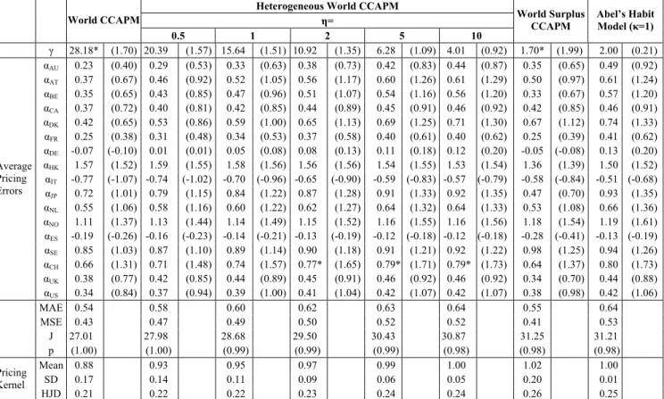
Next, I extend the analysis to all the 17 country indices which are from the G7 countries mentioned above plus Australia, Austria, Belgium, Denmark, Hong Kong, Netherlands, Norway, Spain, Sweden, and Switzerland. The results are reported in Table 3. Similar to the findings in Table 2, Table 3 shows that the more sophisticated models have lower and economically more plausible coefficient estimates of risk aversion than the classic world CCAPM, and the more sophisticated models perform worse than the classic world CCAPM in terms of the goodness-of-the-fit. However, there are two exceptions. First, the estimates for the coefficient of risk aversion are smaller for all models using the 17 country index data than those only using the G7 country index data. Second, the pricing errors for the classic world CCAPM are lower than for the more sophisticated models. This is because in the single assets GMM systems, the estimates for the coefficient of risk aversion in the classic world CCAPM for many non-G7 countriessuch as Australia, Belgium, Denmark, Hong Kong, and Norway are lower (close to 2.0) than the estimates for the G7 countries.12 Therefore, including
11 It is also possible that the results are due to the low power of tests. 12 See Appendix A6.1 in Li (2009) for details.
these countries in the GMM system lowers the risk aversion estimates, which in turn affects pricing errors of different models.
5. Conclusion
In this paper, I study the empirical performance of various consumption models for international equity markets. I use data for 17 MSCI country indices to examine whether consumption variables are related to excess returns on the market indices in different countries. I start with the classic world CCAPM, which assumes that there is a world representative investor and his consumption growth is the only factor in determining asset returns. Then I study the heterogeneous world CCAPM under the framework of Constantinides and Duffie (1996) to investigate whether incomplete consumption risk sharing affects asset pricing. Under the assumption of incomplete consumption risk sharing, country specific factors cannot be diversified away, and therefore idiosyncratic consumption risk must be related to asset returns. I also extend the world CCAPM to two world habit models.
Table 3: Tests of the Euler Equations (17 countries)
Heterogeneous World CCAPM
η= World CCAPM 0.5 1 2 5 10 World Surplus CCAPM Abel’s Habit Model (κ=1) γ 28.18* (1.70) 20.39 (1.57) 15.64 (1.51) 10.92 (1.35) 6.28 (1.09) 4.01 (0.92) 1.70* (1.99) 2.00 (0.21) αAU 0.23 (0.40) 0.29 (0.53) 0.33 (0.63) 0.38 (0.73) 0.42 (0.83) 0.44 (0.87) 0.35 (0.65) 0.49 (0.92) αAT 0.37 (0.67) 0.46 (0.92) 0.52 (1.05) 0.56 (1.17) 0.60 (1.26) 0.61 (1.29) 0.50 (0.97) 0.61 (1.24) αBE 0.35 (0.65) 0.43 (0.85) 0.47 (0.96) 0.51 (1.07) 0.54 (1.16) 0.56 (1.20) 0.33 (0.67) 0.57 (1.20) αCA 0.37 (0.72) 0.40 (0.81) 0.42 (0.85) 0.44 (0.89) 0.45 (0.91) 0.46 (0.92) 0.42 (0.85) 0.46 (0.91) αDK 0.42 (0.65) 0.53 (0.86) 0.59 (1.00) 0.65 (1.13) 0.69 (1.25) 0.71 (1.30) 0.67 (1.12) 0.74 (1.33) αFR 0.25 (0.38) 0.31 (0.48) 0.34 (0.53) 0.37 (0.58) 0.40 (0.61) 0.40 (0.62) 0.25 (0.39) 0.41 (0.62) αDE -0.07 (-0.10) 0.01 (0.01) 0.05 (0.08) 0.08 (0.13) 0.11 (0.18) 0.12 (0.20) -0.05 (-0.08) 0.13 (0.20) αHK 1.57 (1.52) 1.59 (1.55) 1.58 (1.56) 1.56 (1.56) 1.54 (1.55) 1.53 (1.54) 1.36 (1.39) 1.50 (1.52) αIT -0.77 (-1.07) -0.74 (-1.02) -0.70 (-0.96) -0.65 (-0.90) -0.59 (-0.83) -0.57 (-0.79) -0.58 (-0.84) -0.51 (-0.68) αJP 0.72 (1.01) 0.79 (1.15) 0.84 (1.22) 0.87 (1.28) 0.91 (1.33) 0.92 (1.35) 0.47 (0.70) 0.93 (1.35) αNL 0.55 (1.06) 0.58 (1.16) 0.60 (1.22) 0.62 (1.27) 0.64 (1.32) 0.64 (1.33) 0.53 (1.08) 0.66 (1.36) αNO 1.11 (1.37) 1.13 (1.44) 1.14 (1.49) 1.15 (1.52) 1.16 (1.55) 1.16 (1.56) 1.18 (1.54) 1.19 (1.61) αES -0.19 (-0.26) -0.16 (-0.23) -0.14 (-0.21) -0.13 (-0.19) -0.12 (-0.18) -0.12 (-0.18) -0.28 (-0.41) -0.13 (-0.19) αSE 0.85 (1.03) 0.87 (1.10) 0.89 (1.14) 0.90 (1.18) 0.91 (1.21) 0.92 (1.22) 0.98 (1.25) 0.94 (1.26) αCH 0.66 (1.31) 0.71 (1.48) 0.74 (1.57) 0.77* (1.65) 0.79* (1.71) 0.79* (1.73) 0.64 (1.37) 0.80 (1.73) αUK 0.38 (0.77) 0.42 (0.85) 0.44 (0.89) 0.45 (0.91) 0.46 (0.92) 0.46 (0.92) 0.34 (0.70) 0.44 (0.88) Average Pricing Errors αUS 0.34 (0.84) 0.37 (0.94) 0.39 (1.00) 0.41 (1.04) 0.42 (1.07) 0.42 (1.07) 0.38 (0.98) 0.42 (1.06) MAE 0.54 0.58 0.60 0.62 0.63 0.64 0.55 0.64 MSE 0.43 0.47 0.49 0.50 0.52 0.52 0.41 0.53 J 27.01 27.98 28.68 29.50 30.43 30.87 31.25 31.21 p (1.00) (1.00) (0.99) (0.99) (0.99) (0.98) (0.98) (0.98) Mean 0.88 0.93 0.95 0.97 0.99 1.00 1.02 1.00 SD 0.17 0.14 0.11 0.09 0.06 0.05 0.20 0.01 Pricing Kernel HJD 0.21 0.22 0.22 0.23 0.24 0.24 0.26 0.25
Notes: The test assets are the MSCI country indices in 17 countries: Australia (AU), Austria (AT), Belgium (BE), Canada (CA), Denmark (DK), France (FR), Germany (DE), Hong Kong (HK), Italy (IT), Japan (JP), Netherlands (NL), Norway (NO), Spain (ES), Sweden (SE), Switzerland (CH), the UK, and the US. Also see notes to Table 2.
The models are estimated and tested using Hansen’s (1982) GMM. I find that a large risk aversion is needed to explain the equity premium for the classic world CCAPM. The heterogeneous world CCAPM with the cross-country consumption dispersion as the other factor in addition to the world consumption growth has a lower and economically reasonable estimate for the coefficient of consumption risk aversion. The estimate for the coefficient of risk aversion for the world surplus consumption model is also low. However, the overall fit of the model for the more sophisticated models are worse than the one for the classic world CCAPM based on the Hansen J-statistics and the Hansen-Jagannathan distances.
The empirical findings of this study provide new evidence for international asset pricing using consumption models. Under the world representative agent model, which assumes that the market is complete, country-specific consumption risk is perfectly shared among investors and consequently only the aggregate world consumption risk matters for asset pricing (see Cochrane (2001, Ch.3) for the discussion on risk sharing). The findings that the heterogeneous consumption model, relative to the representative agent model, can generate much lower and economically plausible coefficients of relative risk aversion, which suggests that country-specific consumption risk is not fully diversified at the global level and therefore there is a relation between stock returns and the idiosyncratic consumption risk.
References
1] Abel, Andrew B., 1990. “Asset prices under habit formation and catching up with the Joneses”,
American Economic Review Papers and Proceedings 80, pp.38-42.
2] Bekaert, Geert, and Campbell R. Harvey, 1995. “Time-varying world market integration”,
Journal of Finance 50, pp.403-444.
3] Breeden, Douglas T., 1979. “An intertemporal asset pricing model with stochastic consumption and investment opportunities”, Journal of Financial Economics 7, pp.265-296.
4] Campbell, John Y. and John H. Cochrane, 1999. “By force of habit: A consumption-based explanation of aggregate stock market behaviour”, Journal of Political Economy 107, pp.205-251.
5] Chan, K.C., G. Andrew Karolyi, and Rene M. Stulz, 1992. “Global financial markets and the risk premium on U.S. equity”, Journal of Financial Economics 32, pp.137-167.
6] Cho, D. Chinhyung, Cheol S. Eun, and Lemma W. Senbet, 1986. “International arbitrage pricing theory: An empirical investigation”, Journal of Finance 41, pp.313-329.
7] Cochrane, John H., 2001. “Asset Pricing”, Princeton University Press, Princeton, NJ.
8] Constantinides, George M. and Darrel Duffie, 1996. “Asset pricing with heterogeneous consumers”, Journal of Political Economy 104, pp.219-240.
9] Cumby, R.E., 1988. “Consumption risk and international equity returns: Some empirical evidence”, Journal of International Money and Finance 9, pp.182-192.
10] De Santis, Giorgio and Bruno Gerard, 1997. “International asset pricing and portfolio diversification with time-varying risk”, Journal of Finance 52, pp.1811-1912.
11] De Santis, Giorgio and Bruno Gerard, 1998. “How big is the premium for currency risk?”,
Journal of Financial Economics 49, pp.375-412.
12] Dumas, Bernard and Bruno H. Solnik, 1995. “The world price of foreign exchange risk”,
Journal of Finance 50, pp.445-479.
13] Ferson, Wayne E. and Campbell R. Harvey, 1993. “The risk and predictability of international equity returns”, Review of Financial Studies 6, pp.527-566.
14] Hansen, Lars Peter, 1982. “Large sample properties of generalized method of moments estimators”, Econometrica 50, pp.1029-1054.
15] Hansen Lars Peter and Ravi Jagannathan, 1997. “Assessing specification errors in stochastic discount factor models”, Journal of Finance 52, pp.557-590.
16] Harvey, Campbell R., 1991. “The world price of covariance risk”, Journal of Finance 46, pp.111-157.
17] Jorion, Philippe, 1991. “The pricing of exchange rate risk in the stock market”, Journal of Financial and Quantitative Analysis 26, pp.363-376.
18] Karolyi, G. Andrew and Rene M. Stulz, 2003. “Are financial assets priced locally or globally?”, in George M. Constantinides, Milton Harris, and Rene M. Stulz, eds.: The Handbook of the Economics of Finance, North-Holland, Amsterdam.
19] Korajczyk, Robert A. and Claude J. Viallet, 1989. “An empirical investigation of international asset pricing”, Review of Financial Studies 2, pp.553-585.
20] Lettau, Martin and Sydney Ludvigson, 2001a. “Consumption, aggregate wealth, and expected stock returns”, The Journal of Finance 56, pp.815-849.
21] Lettau, Martin and Sydney Ludvigson, 2001b. “Resurrecting the (C)CAPM: A cross-sectional test when risk premia are time varying”, Journal of Political Economy 109, pp.1238-1287. 22] Li, Bin, 2009. “Essays on Consumption-based Asset Pricing Models”, PhD Thesis, the
University of Queensland, Australia.
23] Li, Yuming and Maosen Zhong, 2005. “Consumption habit and international stock returns”,
Journal of Banking & Finance 29, pp.579-601.
24] Li, Yuming and Maosen Zhong, 2009. “International asset returns and exchange rates”,
European Journal of Finance 15, pp.263-285.
25] Lucas, Robert E. Jr., 1978. “Asset prices in an exchange economy”, Econometrica 46, pp.1429-1446.
26] Mehra, Rajnish, 2003. “The equity premium: Why is it a puzzle?”, Financial Analysts Journal
59, pp.54-69.
27] Mehra, Rajnish and Edward C. Prescott, 1985. “The equity premium: A puzzle”, Journal of Monetary Economics 15, pp.145-161.
28] Newey, Whitney K. and Kenneth D. West, 1987. “A simple, positive semi-definite, heteroskedasticity and autocorrelation consistent covariance matrix”, Econometrica 55, pp.703-708.
29] Sarkissian, Sergei, 2003. “Incomplete consumption risk sharing and currency risk premiums”,
Review of Financial Studies 16, pp.983-10.
30] Stehle, Richard, 1977. “An empirical test of the alternative hypotheses of national and international pricing of risky assets”, Journal of Finance 32, pp.493-502.
31] Stulz, Rene M., 1981a. “A model of international asset pricing”, Journal of Financial Economics 9, pp.383-406.
32] Stulz, Rene M., 1981b. “On the effects of barriers to international investment”, Journal of Finance 36, pp.923-934.
33] Wheatley, Simon, 1988. “Some tests of international equity integration”, Journal of Financial Economics 21, pp.177-212.
34] Yogo, Motohiro, 2006. “A consumption-based explanation of expected stock returns", Journal of Finance 61, pp.539-580.