Speculative behaviour and oil price predictability

(1)

Speculative behaviour and oil price predictability

Ekaterini Panopoulou

University of Piraeus, Greece

Theologos Pantelidis

y

University of Macedonia, Greece

Abstract

We develop two- and three-state regime switching models and test their forecasting ability for oil prices. We use the deviations of market oil price from fundamental values as the main explanatory variable in our models, while additional potential predictors enrich our speci…cation. Our …ndings suggest that the regime-switching models are, in general, more accurate than the Random Walk model in terms of both statistical and economic evaluation criteria for oil price forecasts.

JEL Classi…cation: C5; Q4;

Keywords: Oil price; Regime Switching; Forecasting; Deviations from fundamentals.

Correspondence to: Ekaterini Panopoulou, Department of Statistics and Insurance Science, Univer-sity of Piraeus, 80 Karaoli & Dimitriou Str., 18534, Piraeus, Greece. E-mail: [email protected]. Tel: 0030 210 4142728. Fax: 0030 210 4142340.

y_{Theologos Pantelidis, Department of Economics, University of Macedonia, 156 Egnatia Str.,} GR-54006, Thessaloniki, Greece. E-mail: [email protected]. Tel.: 0030 2310 891726. Fax: 0030 2310 891292.

(2)

1 Introduction

Oil price is a key-variable in macroeconomic projections a¤ecting in‡ation and economic activity. Clearly, the predictability of the price of oil is of great interest to policymakers, central banks, CEOs and international investors. Strategic and investment decisions of airline, automobile and energy companies are based on scenarios built on forecasts of the future path of oil price. Even homeowners have in mind some kind of expectations about the future price of oil when deciding about energy-saving investments. Moreover, en-ergy and especially crude oil futures have become widespread investment vehicles among traditional and alternative asset managers, mainly due to their equity-like return, their in‡ation-hedging properties and their role for risk diversi…cation.

The recent surge in oil prices (and other commodities as well) between 2003-2008 has sparked a public debate on the determinants of the price of crude oil. Fundamental-based explanations of oil price movements are attributed to oil supply shocks, oil demand shocks driven by global economic activity, and oil-speci…c demand shocks. Oil supply shocks stem from reduced oil production of oil-exporting regions, while an oil demand shock is mainly caused by unexpected world economic activity. Finally, an oil-speci…c demand shock may be triggered by either changing expectations of oil fundamentals or …nancial speculation. It seems that the literature has reached a consensus on the drivers of the oil price boom until mid-2008. Speci…cally, Hamilton (2009 a,b), Kilian, (2009), Kilian and Hicks (2009), Juvenal and Petrella (2012) and Kilian and Murphy (2013) …nd that the recent oil price rise is mainly attributed to strong oil demand confronting stagnating global oil production. With respect to the oil-speci…c demand shock, this can be decomposed into an oil-speci…c shock which captures changes in oil demand not related to economic activity, and a destabilising …nancial shock. Lombardi and Van Robays (2011) attempt such a decomposition and model the destabilising …nancial shock as a shock that creates a perturbation in the futures market due to increased demand for futures contracts that moves the futures price away from its e¢ cient level. Such …nancial shocks may emerge due to the increasing …nancialisation of oil futures markets measured by the sharp rise in speculative open interest and speculative market shares (see among others Mayer, 2010; Irwin and Sanders, 2011; Tang and Xiong, 2011; CFTC, 2011 Fattouh et al. 2013). However, it is not clear whether the way market participants act is due to lack of a fundamental basis in supply and demand or whether it represents the mechanism by which market fundamentals are incorporated in competitively determined prices. Kilian and Murphy (2013) and Kilian and Lee (2013) argue that …nancialisation in oil futures markets should be modelled as part of the endogenous propagation of shocks to fundamentals rather than an exogenous intervention.

(3)

the case of rational bubbles, these are generated by endogenous responses to the funda-mentals that drive asset prices (Branch and Evans, 2011). The literature mainly focuses on speculative bubbles in the stock market, while the evidence for the oil market is quite scanty. We mention three related studies which explicitly test for speculative bubbles in the oil price by making use of the recently proposed Supremum Augmented Dickey Fuller (SADF) approach (proposed by Phillips et al., 2011). Speci…cally, Gilbert (2010) and Homm and Breitung (2012) cannot detect speculative bubbles in oil prices consistently. By contrast, Phillips and Yu (2011) succeed in detecting explosive behaviour in monthly oil prices normalised by US inventories between March and July 2008. Applying the dura-tion dependence test, Wentet al. (2012) provide further evidence in favour of speculative bubbles in the oil price. Einloth (2009) also attributes part of the oil price movements in recent years to speculation. More recently, Lammerding et al. (2013) draw on the rela-tionship between oil prices and oil dividends and establish a state-space framework from which they extract the bubble component as an unobservable variable. They additionally assume the bubble to evolve over time as a two-state Markov-switching process with two distinct regimes; namely one in which the bubble evolves over time as a stable process and one in which the bubble exhibits explosive dynamics. The authors follow a Bayesian approach, implementing a fully-‡edged Markov-Chain-Monte-Carlo (MCMC) estimation framework and …nd convincing evidence of two distinct bubble episodes in the oil market. In this study, we employ and develop models of speculative behaviour in the oil market building on the existence of a bubble. A word of caution is in order here. We should note that our models do not allow us to attribute the source of a bubble to speci…c characteristics of the oil market and as such we can not infer whether a bubble is based on fundemental or non-fundamental factors. In any event, we do not attempt to discriminate between the two hypotheses. We follow Pindyck (1993) and infer the fundamental value of crude oil from the current and expected discounted convenience yield that accrues from holding inventories based on a non-arbitrage condition between oil spot and futures price. Any deviation of current values from fundamental values is termed ‘bubble’and may summarise a variety of shocks as outlined before. The bubble component can be in one of two or three regimes giving rise to our two- and three-state Regime-Switching (RS) models along the lines of the models developed by Van Norden and Schaller (1993, VNS hereafter) and Brooks and Katsaris (2005, BK hereafter). The authors link speculative behaviour in asset returns to RS models. Speci…cally, VNS show that a two-regime speculative behaviour model, in which the bubble is allowed to switch between a survival and a collapse state has signi…cant explanatory power for stock returns. BK incorporate a third regime in the VNS model to allow for the bubble growing at a steady rate of return bridging the gap between VNS and Evans (1991) who allow for the bubble to

(4)

switch between the dormant and the explosive state. Recently, Shi and Arora (2012, SA hereafter) extended the VNS and BK models to oil prices and found a reasonably good …t of the data along with evidence of a speculative bubble over the late-2008/early-2009 period.

The aforementioned studies focus on the in-sample ability of RS models to capture the dynamics in the price of the asset under scrutiny, ignoring the out-of-sample predictive power of the models. This is the goal of our analysis. To be more speci…c, we augment both the VNS and BK models by adding a variety of variables that serve as predictors of the future dynamics in the oil price and investigate the forecasting performance of these speci…cations. Following BK and SA, we employ the abnormal futures trading volume as a signal of market expectations governing both the mean and the probability equation of the surviving regime. This variable can be thought of as a destabilising …nancial shock in the context of Lombardi and Van Robays (2011). In a similar manner, we incorporate the variables proposed by Kilian and Murphy (2013) which are linked to oil supply shocks, oil demand shocks and oil-speci…c (speculative) demand shocks. Widening the information set (see also Juvenal and Petrella, 2012), we also employ macroeconomic and …nancial variables which act complementarily to measures of economic activity and …nancial conditions.

The forecasting performance of our models is evaluated in both statistical and eco-nomic terms. Ecoeco-nomic evaluation is desirable since the oil market and the commodities markets have attracted the interest of large …nancial institutions, hedge funds and in-vestment funds in general. Commodities are included in inin-vestment portfolios in order to diversify risk (Gorton and Rouwenhorst 2006). To anticipate our key results, the RS models appear to generate more accurate forecasts of the oil price, in both statistical and economic evaluation terms, relative to the Random Walk (RW) benchmark. Speci…cally, the RS models considered in this study outperform the RW model and the improvement in the accuracy of the oil price forecasts is statistically signi…cant in all cases. Moreover, their superiority over the RW model is even stronger in economic evaluation terms. Fi-nally, many of the predictors examined in this study appear to improve the forecasting accuracy of the RS models.

In the literature there are many studies that focus on oil forecasts but, to the best of our knowledge, none of them employs the class of RS models considered in our study. For example, Knetsch (2007) generates forecasts of the price of oil by means of a convenience yield forecasting model. His approach leads to more accurate forecasts of oil prices com-pared to direct forecasts from futures prices of the commodity but fails to beat the RW model (based on the root mean squared error criterion). Similarly, Alquist and Kilian (2010) provide evidence that forecasts from oil futures prices tend to be less accurate than

(5)

forecasts from the RW model. Wu and McCallum (2005) argue that the accuracy of oil price forecasts can be improved by taking into account the relationship between current spot and futures prices instead of considering only the raw futures price. Baumeister and Kilian (2012) organise a forecasting exercise in real-time terms and provide evidence sup-porting the ability of Vector AutoRegressive (VAR) models to generate reliable forecasts of the real price of oil, while Baumeister and Kilian (2013) examine the predictability of the oil price from a central banker’s point of view. Finally, Alquist et al. (2011) provide a stimulating review on the predictability of oil price.

The remainder of this paper is organised as follows. Section 2 introduces the Regime-Switching models used in this study, describes our approach to construct fundamental values and outlines the rationale behind the choice of predictors included in our models. Section 3 describes the dataset and reports the empirical …ndings of the study. Finally, Section 4 concludes.

2 Economic modelling and econometric speci…cation

In this section, we initially provide a brief description of the three-state RS model of BK, which we augment with various predictors for the price of oil. The selection of these predictors is based on the existing literature on the determinants of oil price. We also describe two restricted versions of the three-regime model which we consider in our study and apply an arbitrage relation to calculate the convenience yield that allows us to obtain fundamental values.

2.1 Speculative behaviour and regime-switching models

Consider a simple asset pricing model where risk-neutral investors choose between holding an asset that yields (1 +r) and a risky asset, in our case oil. The investors’…rst order conditions imply that the price of the asset, Pt is given as follows:

Pt= 1

1 +r(Et(Pt+1+Dt)

where Dt is some payo¤ in the form of dividends (stock market), convenience yield (oil

and commodity markets), etc. One possible solution of the above equation de…nes the fundamental value of the asset, P_tf, as follows:

P_tf = 1

X

k=0

(6)

All other prices are said to be bubbly and the bubble component, (Bt); is de…ned as1

Bt =Pt Ptf

We assume that the expected size of the bubble in the next period can be generated from one of three regimes: a deterministic (dormant) regime (D), a surviving explosive regime (S) and a collapsing explosive regime (C) giving rise to a three regime model of speculative behaviour. As BK suggest, while several variables may prove signi…cant in classifying the behaviour of the asset of interest, the relative size of the bubble is expected to play a predominant role.

If the bubble is in regime D, investors believe that it will continue to grow at a constant rate (1 +rf) :

Et(Bt+1 jWt+1 =D) = (1 +rf)Bt (1)

where Bt is the size of the bubble (the di¤erence between the actual and fundamental

values) at time t, rf is a constant discount rate and Wt (or Statet) is an unobserved

variable that determines the regime. In this regime, the probability of collapse is negligible and investors do not demand an excess return for this. The probability of being in regime D in time t+ 1 is denoted by _t and depends on the relative size of the bubble (bt) and

other observed variables at time t. Even when the bubble is in the dormant regime, investors attach some probability in the bubble entering the explosive state by either surviving or collapsing. The probability of the explosive state is given by 1 _t and in this explosive state the probabilities of the two underlying regimes (Survive or Collapse) are denoted by qt and (1 qt), respectively. In other words, the probability of being in

each state is as follows:

Pr(Statet+1 = D) = t

Pr(Statet+1 = S) = (1 t)qt Pr(Statet+1 = C) = (1 t)(1 qt)

In the collapsing regime, the expected size of the bubble is given by

Et(Bt+1 jWt+1 =C) = g(bt)Pt (2)

whereg(bt)is a continuous and everywhere di¤erentiable function such thatg(0) = 0and 0 @g(bt)=@bt 1 +rf, bt is the relative size of the bubble (bt = Bt=Pt) and Pt is the

1_{The fundamental component, and consequently the bubble component, is calculated by means of}

the present value model of rational commodity pricing put forward by Pindyck (1993). Please refer to Subsection 2.2 for details on the calculation of the bubble.

(7)

actual asset price at time t:2 _{Finally, the expected value of the bubble in the surviving}

regime is given by:3

Et(Bt+1 jWt+1 =S) = (1 +rf) qt Bt (1 qt) qt g(bt)Pt (3)

After some manipulation, the expected values in equations (1)-(3) can be written in terms of expected gross total returns of the next period, Rt+1 as follows:

Et(Rt+1 j Wt+1 =D) = (1 +rf) (4) Et(Rt+1 j Wt+1 =C) = (1 +rf)(1 bt) +g(bt) (5) Et(Rt+1 j Wt+1 =S) = (1 +rf) + (1 qt) qt [(1 +rf)bt g(bt)] (6)

where Rt+1 = (Pt+1 +Dt+1)=Pt: Equations (4)-(6) suggest that in the dormant regime

investors expect a gross return equal to the required rate of return on the bubble-free asset, while in the surviving and collapsing regimes the gross return is a function of both the required rate of return and the relative size of the bubble.

We now turn to modelling the probabilities t and qt which as already mentioned are

negative functions of the bubble and speci…cally the absolute value of the bubble, _jbtj,

since we allow for both negative and positive deviations. In order to model the probability of being in the dormant regime in the next time period, we follow BK and include the absolute value of the spread, (st)de…ned as the average 12-month actual returns minus the

absolute value of the average 12-month returns of the estimated fundamental values. The intuition behind this speci…cation is quite clear. When investors observe large spreads, i.e. larger average returns than average fundamental returns, they tend to believe that the bubble has entered the explosive state and the probability of being in the dormant state falls. In order to ensure that the estimated probability is bounded between 0 and 1, we adopt a Probit speci…cation. Under this setting, the probability of being in the dormant regime in the next time period is given by:

Pr(Statet+1 =D) = t = ( 0 + 1jbtj+ 2st) (7)

where is the cumulative density function of the standard normal distribution.

The basic assumption of the speculative bubble models is that the arrival of news may fuel a bubble collapse, which is often viewed as a random occasion that causes investors to liquidate their position at a certain point in time. Although investors observe the

2_{Please note that the function}_g₍_b

t)is for theoretical illustration and is not imposed on the data. 3_{Equation (3) is derived from equations (1) and (2) employing the probabilities of the two underlying}

(8)

built-up of the bubble and expect the bubble to collapse, they cannot precisely estimate the time of the collapse. BK propose that abnormally high trading volume is a signal of changing market expectations about the future of a speculative bubble. We enrich the BK speci…cation with a set of observable/macroeconomic variables, which we assume that investors monitor and which act as a signal of changing economic conditions and as a result changing market expectations that help them …nd the optimal exit-time from the market. Our set of signalling indicators comprises of variables typically employed in oil price determination.4 Under this setting, we model the probability of survival as a function of both the bubble size and one of the indicators (zt) as follows:

qt= ( q0 + q1jbtj+ q2zt) (8)

The model described in equations (4) - (8) is highly nonlinear and in order to linearise it we take the …rst order Taylor Series expansion of (4)-(6) around an arbitraryb0 and z0.

The resulting linear regime switching model is given by the following set of equations:

BK extended (9) Rd;t+1 = d0+"d;t+1; where "d;t+1 N(0; 2d) Rs;t+1 = s0 + s1bt+ s2zt+"s;t+1; where "s;t+1 N(0; 2s) Rc;t+1 = c0+ c1bt+"c;t+1; where "c;t+1 N(0; 2c) Pr(Statet+1 =D) = t = ( 0 + 1jbtj+ 2st) qt= ( q0 + q1jbtj+ q2zt)

The BK-extended model is estimated by maximising the associated likelihood func-tion, given by the following formula:

Y t [_f _t_g' Rt+1 d0 d 1 d ] +f1 tg fqtg' Rt+1 s0 s1bt s2zt s 1 s + (10) +_f1 _t_{g f}1 qtg' Rt+1 c0 c1bt c 1 c ]

where ' is the standard normal probability density function (pdf).

Obviously, when the signal indicator variable coincides with abnormal trading volume, the BK-extended speci…cation coincides with the BK model. Furthermore, if we set the probability of being in the dormant regime equal to zero and exclude all explanatory 4_{Additional information about the variables-predictors we use in our analysis is provided in Subsection}

(9)

variables (other than bt) from the speci…cation, our model reduces to the original VNS

model, which serves as the natural benchmark in our analysis and is outlined by the following set of equations.

V N S (11)

Rs;t+1 = s0+ s1bt+"s;t+1; where "s;t+1 N(0; 2s)

Rc;t+1 = c0+ c1bt+"c;t+1; where "c;t+1 N(0; 2c) Pr(Statet+1 =S) =qt= ( q0 + q1jbtj)

To gauge the in‡uence/signi…cance of the candidate indicator variables, we also aug-ment the VNS model by adding the signal variable zt in both the mean equation for the

survival regime and the probability of survive, qt; as follows:

V N S extended (12)

Rs;t+1 = s0 + s1bt+ s2zt+"s;t+1; where "s;t+1 N(0; 2s)

Rc;t+1 = c0+ c1bt+"c;t+1; where "c;t+1 N(0; 2c) Pr(Statet+1 =S) = qt= ( q0 + q1jbtj+ q2zt)

As previously, VNS and VNS-extended models are estimated by the associated likeli-hood functions.

2.2 Bubble calculation

The fundamental value of the oil price is de…ned as the sum of the current and expected convenience yield that accrues from holding inventories in the same way that the dividend yield is employed to estimate the fundamental value in the stock market. Following Pindyck (1993), SA and Lammerding et al. (2013), we use the futures prices in order to measure the convenience yield of actively traded storable commodities. More in detail, letYt;1 denote the current monthly convenience yield, rtthe risk-free interest rate, Pt the

spot price of oil andFt+1 the futures price. Then, the convenience yield is calculated by

the following non-arbitrage condition

Yt;1 = (1 +rt)Pt Ft+1

which simply states that in equilibrium the futures price must equal the spot price (ad-justed for opportunity costs) and the bene…ts of holding the commodity. Once we obtain the convenience yield, we follow Campbell and Shiller (1987) in order to calculate the fundamental value and the bubble size by employing the convenience yield instead of

(10)

the dividend yield. Speci…cally, the Campbell and Shiller model allows for predictable variation in expected convenience yields and is based on a simple present value model of stock prices. If the present value model of oil spot prices

Pt =Et 1 X i=0 ( 1 1 +r) i_Y t;i

were true, then a linear function of current prices and convenience yields would be the op-timal linear forecast of future convenience yields. This linear function, namely the spread (St), is de…ned as the di¤erence between price and a multiple of current convenience yield

and can be estimated through a VAR representation for the change in convenience yields and the spread itself. More in detail, the spread (St) and the implied bubble measure

(bt) are given by the following formulas

St=Pt 1 +r r Dt= 1 +r r 1 X i=0 ( 1 1 +r) i_E t( Dt+i) bt = 1 St+ ((1 +r)=r) Dt 1 Pt

We set the discount rate equal to

r= 1

Pt=Dt 1

to ensure that the spread has a zero mean over the whole sample.

2.3 Choice of indicator variables

In this section, we outline the rationale behind the choice of the signal/indicator variables employed in the extended BK and VNS models. As already mentioned, BK employ the abnormal futures trading volume as a signal of market expectations governing both the mean and the probability equation of the surviving regime. This variable can be thought of as a destabilising …nancial shock in the context of Lombardi and Van Robays (2011). Drawing from the structural vector autoregressive model of the global market for crude oil proposed by Kilian and Murphy (2013), we also employ variables linked to demand and supply shocks in the oil market. Since these models produce empirically plausible estimates of the impact of demand and supply shocks on the real price of oil, they may also have value for forecasting the real price of oil. The variables in this model include the percent change in global crude oil production, a measure of global real activity and the change in global above-ground crude oil inventories. Global crude oil production serves as the ‡ow supply shock and global real activity, which is the dry cargo

(11)

shipping rate index developed by Kilian (2009), serves as the ‡ow demand shock and represents unexpected ‡uctuations in the global business cycle. Finally, the speculative demand shock, which is a shock to the demand for oil inventories arising from forward-looking behaviour of market participants is proxied by crude oil inventories. Widening the information set, we also employ macroeconomic and …nancial variables which act complementarily to measures of economic activity and …nancial conditions. First of all, following Juvenal and Petrella (2012), we consider an alternative measure of economic activity proxied by US industrial production. Admittedly, this variable is just a weak substitute for global economic activity, however the …rst factor the authors extract from a large dataset of 151 variables of the G7 countries loads primarily on industrial production. More importantly, this measure of economic activity is found to summarise aggregate business cycle conditions, while the proxy proposed by Kilian (2009) is more forward looking measure summarising aggregate demand and loading heavily on US personal consumption. The remaining variables we employ are mainly US variables and mainly contributing to the …rst factor with the exception of the US monetary base (M1) that is linked to the second factor. Anzuini et al. (2010) highlight that expansionary monetary policy may have fuelled oil price increases, but also report that it appears to exert its impact through expectations of higher in‡ation and growth rather than on the ‡ow of global liquidity into oil futures markets. By no means is this list of variables exhaustive. For a detailed list of variables determining oil prices, the reader is referred to Alquist et al. (2011) and Juvenal and Petrella (2012).

3 Empirical …ndings

3.1 Data

Our dataset consists of monthly observations from January 1985 to December 2010. Pt

and Ft+1 are the prices of the nearest-month and the next-to-nearest month West Texas

Intermediate (WTI) futures contract taken from the US Energy Information Adminis-tration, respectively. The risk free interest rate is the 3-month Treasury Bill rate and the US Consumer Price Index (CPI) is employed to de‡atePt and Yt;1 (both taken from

the Federal Reserve Economic Data, FRED). The futures trading volume data is based on nearest-month futures contracts of WTI (DataStream International)5_{. Following SA,}

abnormal trading volume is calculated as the percentage deviation of last months’volume from the 6-month moving average. Our measure of ‡uctuations in global real activity is the dry cargo shipping rate index developed in Kilian (2009). This real activity index is 5_{The data necessary for the calculation of the bubble along with the abnormal trading volume were}

(12)

a business cycle index, designed to capture shifts in the global use of industrial commodi-ties, and stationary by construction.6 _{Data on global crude oil production are available}

in the Monthly Energy Review of the Energy Information Administration (EIA). These data include lease condensates, but exclude natural gas plant liquids and are expressed in percent changes. Given the lack of data on crude oil inventories for other countries, we follow Hamilton (2009a) and Kilian and Murphy (2013) in using the data for total U.S. crude oil inventories provided by the EIA, scaled by the ratio of OECD petroleum stocks over U.S. petroleum stocks, also obtained from the EIA. We express the resulting proxy for global crude oil inventories in percent changes. Finally, the US macroeco-nomic/…nancial indicator variables are sourced from the FRED database. Speci…cally, we employ the long-term (DGS10) and short-term interest rate (GS3M), the growth rate in industrial production (INDPRO), the CPI (CPIAUCSL) and PPI (PPIACO) in‡ation rate, the growth in M1 money stock (M1) and the unemployment rate (UNRATE).

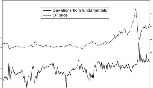
Figure 1 presents the price of oil together with the calculated deviations from funda-mental values. We observe signi…cant negative deviations in the late ’80s and late ’90s. On the other hand, there seems to be a noteworthy positive bubble in the last two years of our sample.

[FIGURE 1 AROUND HERE]

3.2 Forecasting - Statistical evaluation

We focus on one-period ahead forecasts and organise the forecast exercise in real-time terms, i.e. we obtain a forecast for period t + 1 using all available information up to period t. All models and the deviations from fundamentals are re-estimated recursively and the …rst estimation sample ends in December 2002, leaving the last 8 years of our sample (about one third of the available observations) for the out-of-sample evaluation period.

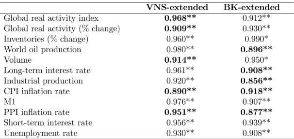
Table 1 reports the ratio of the Mean Squared Forecast Error (MSFE) of each one of the RS models over the MSFE of the RW model.7 _{A ratio below unity indicates the}

superiority of our RS model over the RW model. In all cases, the RS models outperform the benchmark and the MSFE ratios are usually well below unity. In the case of the simple VNS model that does not contain any explanatory variables (other than the deviations from fundamentals), the MSFE ratio equals 0.929. When we enrich the speci…cation of the RS model with one of the twelve predictors considered in our analysis (VNS-6_The _index _is _available _from _Lutz _Kilian’s _website:

http://www-personal.umich.edu/~lkilian/paperlinks.html

7_{We consider both the RW model with and without a drift. The former produces more accurate}

forecast than the latter. We choose to compare our RS models with the optimal RW model (i.e. the one that includes a drift).

(13)

extended model), the MSFE ratios range from 0.89 (CPI in‡ation rate) to 0.98 (world oil production) depending on the predictor. Substantial improvements in the forecasting performance of the RS models are observed when we allow for a third regime in our speci…cation (BK-extended model). In this case, the MSFE ratios are usually around 0.9 with a minimum value of 0.856 when we use the industrial production as a predictor.

Among the twelve variables considered in our analysis, the growth rate of industrial production and the in‡ation rate seem to be the optimal predictors (in the context of our RS models) for the price of oil. Comparing the relative forecasting accuracy of the VNS-extended and the BK-extended models, we observe that, in general, the three-state RS models produce lower MSFEs than the two-state ones.

[TABLE 1 AROUND HERE]

Turning to the statistical signi…cance of the predictive power of our models and given that we are interested in comparing the forecasting performance of nested models, we apply the methodology developed by Clark and West (2006, 2007). Speci…cally, letRRW;t

and RRS;t denote the forecasts forRt obtained from the RW and RS model respectively.

Given a sequence of P forecasts, we …rst calculate:

ft= (Rt RRW;t)2 (Rt RRS;t)2+ (RRW;t RRS;t)2; t= 1;2; :::; P

The test statistic of Clark and West is given by the standardt statisticof the regression of ft on a constant. Clark and West (2006, 2007) recommend using 1.282 and 1.645 for

a 0.10 and 0.05 test, respectively. We should note that this is a one-sided test. Clark and West show that under the null hypothesis of equal MSFE, the unrestricted model (the RS model in our case) should generate larger MSFE than the restricted one (RW in our case). The intuition behind this argument is that since under the null hypothesis the additional parameters of the unrestricted model do not help predictions, in …nite samples this model loses e¢ ciency due to the estimation of these parameters that introduces noise into the forecasts. This in‡ates the MSFE of the model. Therefore, even if the restricted model generates smaller MSFE than the unrestricted one, we should not consider this as prima facie evidence of superiority of the former over the latter.

The …ndings are presented in Table 1 where the asterisks next to the calculated MSFE ratio denote rejection of the null hypothesis at the relevant con…dence level. The results clearly suggest that the superiority of the RS model relative to the RW model is always statistically signi…cant. We go one step further and examine whether the inclusion of a predictor, zt, in our RS models improves the accuracy of forecasts by comparing the

(14)

model that contains no predictors. Entries in bold in Table 1 indicate cases where the extended RS model generates forecasts that are statistically more accurate compared to those from the simple VNS model. Both the VNS-extended model and the BK-extended model outperform the simple VNS model in …ve out of twelve cases. Among the predictors under scrutiny, the CPI and PPI in‡ation rates achieve the best forecasting performance of the RS models considered in this study.

3.3 Economic evaluation

We also perform an economic evaluation of the forecasts of our RS models based on (i) the utility-based approach initiated by West et al. (1993) and (ii) the manipulation-proof performance measure proposed by Goetzmann et al. (2007). We brie‡y describe the two approaches. Consider a US investor who dynamically rebalances her portfolio every month. Her portfolio choice problem is how to allocate wealth between a risk-free asset yielding interest rate it,8 and the risky future contract on the price of oil. In a

mean-variance framework and given a speci…c Relative Risk Aversion (RRA) coe¢ cient, , that controls the investor’s appetite for risk (Campbell and Viceira, 2002), she chooses the optimal weight on the risky asset in a standard maximisation problem resulting in a portfolio return over the out-of-sample period equal to, say,rp;t+1. Then, over the forecast

evaluation period the investor with initial wealth of Wo = 1$ realises an average utility

of U = 1 P P_X1 t=0 (rp;t+1 2(rt+1 rt+1) 2₎ ₍₁₃₎

A risk-averse investor will be willing to pay a performance fee, denoted by , for switching from the portfolio constructed based on RW forecasts to a portfolio based on our proposed RS forecasts if the latter are superior to the former. In our set-up the performance fee is calculated as the di¤erence between the realised utilities as follows:

1 P P 1 X t=0 (r_p;tRS₊₁ 2(rt+1 rt+1) 2_{) =} 1 P P 1 X t=0 (r_p;tRW₊₁ 2(rt+1 rt+1) 2_{) =} ) (14) = URS URW

Positive values of suggest superior predictive ability of the RS model against the RW benchmark.

On the other hand, the manipulation-proof performance measure, M(Rp); can be

in-terpreted as a portfolio’s premium return after adjusting for risk and it remedies potential caveats associated with the popular Sharpe ratio such as the e¤ect of non-normality, the

(15)

underestimation of the performance of dynamic strategies and the choice of utility func-tion. The di¤erence, , between the M(Rp)s of competing models is employed to assess

the most valuable model. This measure is de…ned as

M(Rp) = 1 1 ln ( 1 P P 1 X t=0 1 +rp;t+1 it 1 ) (15) = M(Rp)RS M(Rp)RW

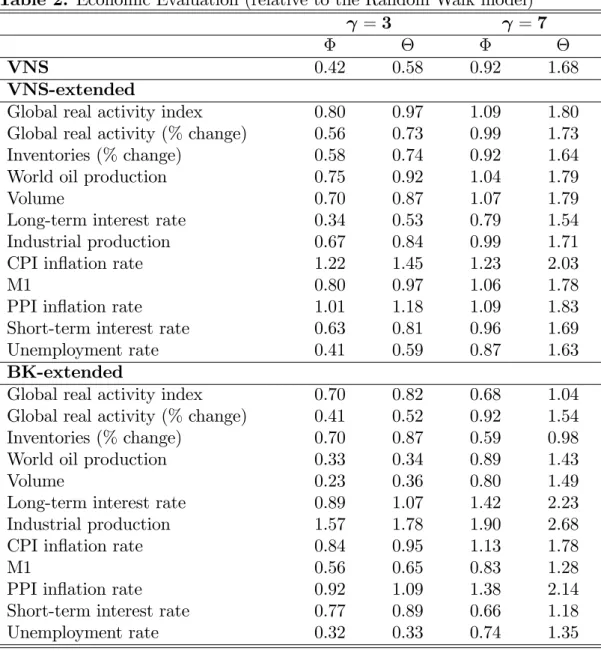
Table 2 reports both economic evaluation measures in monthly percentage points. We do not allow short-selling and we consider two di¤erent values for the RRA coe¢ cient ( = 3 and = 7). In general, both measures produce qualitatively similar results. We always observe signi…cant gains in economic terms for the investor who is willing to switch from the benchmark RW model to one of the RS models. For example, when = 3, the utility gain equals 0.42% for the simple VNS model, while the average utility gains for the VNS-extended and the BK-extended models are 0.71% and 0.69%, respectively. We observe the highest utility gain in the case of the three-sate model that includes the industrial production as a predictor. In this case, equals 1.57% which corresponds to a 18.84% gain in annual terms. Contrary to our …ndings for the statistical evaluation of our forecasts, the VNS-extended model seems to generate slightly higher utility gains relative to the BK-extended model. It is also interesting to note that models with low MSFE ratios do not necessarily generate higher gains in economic terms. For example, in the case of the three-state model that includes the world oil production, the MSFE ratio relative to the RW model is as low as 0.896, while both economic evaluation measures are pretty low ( = 3). In general, as the RRA coe¢ cient increases, utility gains of the RS models relative to the RW model become more pronounced.

[TABLE 2 AROUND HERE]

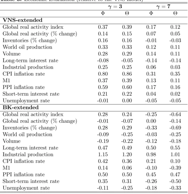
Finally, we repeat the economic evaluation procedure replacing RW with VNS. In other words, we compare VNS-extended and BK-extended with the VNS model. In this way, we investigate whether the inclusion of a predictor in the RS speci…cation produces any bene…ts in economic terms. These …ndings are reported in Table 3. In the majority of cases, we observe positive values of and , reaching 1.15% and 1.20%, respectively, in the case of the BK-extended model that includes the growth rate of the industrial production as a predictor ( = 3). In general, the bene…ts from VNS-extended are higher compared to those from BK-extended.

(16)

4 Conclusions

We develop two- and three-state Regime-Switching (RS) models and test their forecasting ability for oil prices. Taking advantage of the deviations we periodically observe between the market price of oil and its fundamental value, our models relate the expected gross return in the oil price to deviations from fundamentals and an additional explanatory variable. Speci…cally, we compare the predictive power (in both statistical and economic evaluation terms) of twelve alternative macroeconomic/indicator variables assuming a forecast horizon of one month. Our …ndings indicate substantial bene…ts, in terms of forecasting accuracy, when RS models are employed relative to the Random Walk (RW) benchmark, especially in economic evaluation terms. Moreover, the RS models enriched with one of the predictors proposed in this study often outperform simple RS models that contain no predictors (other than deviations from fundamentals).

Our …ndings reveal that speculative behaviour models can be used to generate reliable out-of-sample forecasts for the price of oil. The analysis opens routes for future research to other commodities, such as gold and wheat. It would also be very interesting to investigate whether combination of forecasts from various models can lead to additional accuracy gains.

(17)

References

[1]Alquist, R., Kilian, L., 2010. What do we learn from the price of crude oil futures?,

Journal of Applied Econometrics, 25, 539-573.

[2]Alquist, R., Kilian, L., Vigfusson, R.J., 2011. Forecasting the price of oil, forthcoming in: G. Elliott and A. Timmermann (eds.), Handbook of Economic Forecasting, 2, Amsterdam: North-Holland.

[3]Anzuini, A., Lombardi, M.J., Pagano, P., 2010. The impact of monetary policy shocks on commodity prices, ECB Working Paper 1232.

[4]Baumeister, C., Kilian, L., 2012. Real-time forecasts of the real price of oil, Journal of Business and Economic Statistics, 30(2), 326-336.

[5]Baumeister, C., Kilian, L., 2013. What central bankers need to know about forecasting oil prices, Bank of Canada, Working Paper 2013-15.

[6]Branch, W.A., Evans, G.W., 2011. Learning about risk and return: a simple model of bubbles and crashes, American Economic Journal: Macroeconomics 3, 159-191. [7]Brooks, C., Katsaris, A., 2005. A three-regime model of speculative behaviour:

Mod-elling the evolution of the S&P 500 composite index, The Economic Journal, 115, 767–797.

[8]Campbell, J.Y., Shiller, R.J., 1987. Cointegration and tests of present value models,

The Journal of Political Economy 95, 1062–1088.

[9]Campbell, J.Y., Viceira, L., 2002. Strategic asset allocation, Oxford: Oxford Univer-sity Press.

[10]Clark, T.E., West, K.D., 2006. Using out-of-sample mean squared prediction errors to test the martingale di¤erence hypothesis, Journal of Econometrics, 135, 155-186. [11]Clark, T.E., West, K.D., 2007. Approximately normal tests for equal predictive

accu-racy in nested models, Journal of Econometrics, 138 (1), 291–311.

[12]CFTC, 2011. CFTC commitments of traders, US commodity futures trading commis-sion, Washington, DC.

[13]Einloth, J.T., 2009. Speculation and recent volatility in the price of oil,Social Science Research Network (SSRN) Working Paper.

[14]Evans, G.W., 1991. Pitfalls in testing for explosive bubbles in asset prices,American Economic Review, 81, 922-930.

[15]Fattouh, B., Kilian, L., Mahadeva, L., 2013. The role of speculation in oil markets: What have we learned so far?, Energy Journal, 34 (3), forthcoming.

[16]Gilbert, C.L., 2010. Speculative in‡uences on commodity futures prices 2006–2008,

United Nations Conference on Trade and Development (UNCTAD) Discussion Paper No. 197.

(18)

[17]Goetzmann, W., Ingersoll, J., Spiegel, M., Welch, I., 2007. Portfolio performance ma-nipulation and mama-nipulation-proof performance measures, Review of Financial Stud-ies, 20, 1503-1546.

[18]Gorton, G., Rouwenhorst, K.G, 2006. Facts and fantasies about commodity futures,

Financial Analysts Journal, 62(02), 47–68.

[19]Hamilton, J.D., 2009a. Causes and consequences of the oil shock of 2007–2008, Brook-ings Papers on Economic Activity, 215-259.

[20]Hamilton, J.D., 2009b. Understanding crude oil prices, Energy Journal, 30 (2), 179– 206.

[21]Homm, U., Breitung, J., 2012. Testing for speculative bubbles in stock markets: A comparison of alternative methods.Journal of Financial Economics, 10 (1), 198–231. [22]Irwin, S.H., Sanders, D.R., 2011. Index funds, …nancialization and commodity futures

markets, Applied Economic Perspectives and Policy,33, 1-31.

[23]Juvenal, L., Petrella, I., 2012. Speculation in the oil markets, Working Paper 2011-027E (revised June 2012), Federal Reserve Bank of St. Louis, Working Paper Series.

[24]Kilian, L., 2009. Not all oil price shocks are alike: disentangling demand and supply shocks in the crude oil market, American Economic Review,99 (3), 1053–1069. [25]Kilian, L., Hicks, B., 2009. Did unexpectedly strong economic growth cause the oil

price shock of 2003–2008?, Journal of Forecasting, forthcoming.

[26]Kilian, L., Lee, T.K., 2013. Quantifying the speculative component in the real price of oil: The role of global oil inventories, Journal of International Money and Finance, forthcoming.

[27]Kilian, L., Murphy, D., 2013. The role of inventories and speculative trading in the global market for crude oil, Journal of Applied Econometrics, forthcoming.

[28]Knetsch, T.A., 2007. Forecasting the price of oil via convenience yield predictions,

Journal of Forecasting, 26, 527-549.

[29]Lammerding, M., Stephan, P, Trede, M., Wil‡ing, B., 2013. Speculative bubbles in recent oil price dynamics: Evidence from a Bayesian Markov-switching state-space approach, Energy Economics, 36, 491-502.

[30]Lombardi, M.J., Van Robays, I., 2011. Do …nancial investors destabilize the oil price?, Working Paper Series No. 1346. European Central Bank, Frankfurt/Main.

[31]Mayer, J, 2010. The …nancialization of commodity markets and commodity price volatility, In Dullien, S., Kotte, D.J., Marquez, A. Priewe, J. (Eds.) The Financial and Economics Crisis of 2008-2009 and Developing Countries. UNCTAD, New York and Geneva.

(19)

[32]Pindyck, R.S., 1993. The present value model of rational commodity pricing, The Economic Journal, 103, 511-530.

[33]Phillips, P.C.B., Yu, J., 2011. Dating the timeline of …nancial bubbles during the subprime crisis, Quantitative Economics, 2 (3), 455–491.

[34]Phillips, P.C.B., Wu, Y., Yu, J., 2011. Explosive behavior in the 1990s Nasdaq: When did exuberance escalate asset values?, International Economic Review, 52, 201-226. [35]Shi, S., Arora, V., 2012. An application of models of speculative behaviour to oil

prices, Economics Letters 115, 469–472.

[36]Tang, K., Xiong, W., 2011, Index investment and …nancialization of commodities,

Financial Analysts Journal 68 (6), 54-74

[37]van Norden S., Schaller, H., 1993. The predictability of stock market regime: Evidence from the Toronto stock exchange, Review of Economics and Statistics 75, 3, 505–510.

[38]Went, P., Jirasakuldech, B., Emekter, R., 2012. Rational speculative bubbles and commodities markets: Application of duration dependence test, Applied Financial Economics, 22 (7), 581–596.

[39]West, K., Edison, H., Cho, D., 1993. A utility-based comparison of some models of exchange rate volatility, Journal of International Economics, 35, 23-46.

[40]Wu, T., McCallum, A., 2005. Do Oil Futures Prices Help Predict Future Oil Prices?,

(20)

-0.8 -0.4 0.0 0.4 0.8 1.2 0 40 80 120 160 86 88 90 92 94 96 98 00 02 04 06 08 10

Deviations from fundamentals Oil price

(21)

Table 1. Mean Squared Forecast Errors (MSFEs) Ratios and Statistical Evaluation

VNS = 0.929**

VNS-extended BK-extended

Global real activity index 0.968** 0.912**

Global real activity (% change) 0.909** 0.930**

Inventories (% change) 0.960** 0.990*

World oil production 0.980** 0.896**

Volume 0.914** 0.950*

Long-term interest rate 0.961** 0.908**

Industrial production 0.920** 0.856**

CPI in‡ation rate 0.890** 0.918**

M1 0.976** 0.907**

PPI in‡ation rate 0.951** 0.877**

Short-term interest rate 0.956** 0.939**

Unemployment rate 0.930** 0.908**

Notes: The table reports the ratio of the Mean Squared Forecast Error (MSFE) of

the Regime-Switching (RS) model over the MSFE of the Random Walk (RW) model. (**) and (*) denote the superiority in statistical terms of the RS model relative to the RW model at a 5% and 10% con…dence level respectively. Entries in bold indicate the superiority in statistical terms of the corresponding model relative to the VNS model at a 10% con…dence level.

(22)

Table 2. Economic Evaluation (relative to the Random Walk model)

=3 =7

VNS 0.42 0.58 0.92 1.68

VNS-extended

Global real activity index 0.80 0.97 1.09 1.80

Global real activity (% change) 0.56 0.73 0.99 1.73

Inventories (% change) 0.58 0.74 0.92 1.64

World oil production 0.75 0.92 1.04 1.79

Volume 0.70 0.87 1.07 1.79

Long-term interest rate 0.34 0.53 0.79 1.54

Industrial production 0.67 0.84 0.99 1.71

CPI in‡ation rate 1.22 1.45 1.23 2.03

M1 0.80 0.97 1.06 1.78

PPI in‡ation rate 1.01 1.18 1.09 1.83

Short-term interest rate 0.63 0.81 0.96 1.69

Unemployment rate 0.41 0.59 0.87 1.63

BK-extended

Inventories (% change) 0.70 0.87 0.59 0.98

Volume 0.23 0.36 0.80 1.49

CPI in‡ation rate 0.84 0.95 1.13 1.78

M1 0.56 0.65 0.83 1.28

PPI in‡ation rate 0.92 1.09 1.38 2.14

Unemployment rate 0.32 0.33 0.74 1.35

Notes: stands for the Relative Risk Aversion coe¢ cient. Entries correspond to

the value of and when we compare the Regime-Switching (RS) model relative to the Random Walk (RW) model. The performance fee, , is the fraction of the wealth which when subtracted from the RS proposed portfolio returns equates the average utilities of the competing model (i.e. the RS and the RW models). If our proposed RS model does not contain any economic value, the performance fee is negative ( 0), while positive values of the performance fee suggest superior predictive ability against the RW benchmark. is the di¤erence between the manipulation-proof performance measure of competing models (RS and RW). Both and and are reported in percentage points on a monthly basis.

(23)

Table 3. Economic Evaluation (relative to the VNS model)

=3 =7

VNS-extended

Inventories (% change) 0.16 0.16 -0.01 -0.03

Volume 0.28 0.29 0.14 0.11

Long-term interest rate -0.08 -0.05 -0.14 -0.14

CPI in‡ation rate 0.80 0.86 0.31 0.35

M1 0.37 0.39 0.13 0.11

PPI in‡ation rate 0.59 0.60 0.17 0.16

Unemployment rate -0.01 0.00 -0.05 -0.05

BK-extended

Global real activity index 0.28 0.24 -0.25 -0.64

Global real activity (% change) -0.01 -0.07 0.00 -0.14

Inventories (% change) 0.28 0.29 -0.33 -0.69

World oil production -0.09 -0.25 -0.03 -0.25

Volume -0.19 -0.22 -0.12 -0.18

CPI in‡ation rate 0.42 0.36 0.21 0.10

M1 0.14 0.06 -0.10 -0.39

PPI in‡ation rate 0.50 0.50 0.45 0.47

Short-term interest rate 0.35 0.31 -0.26 -0.50

Unemployment rate -0.11 -0.25 -0.18 -0.33

Notes: stands for the Relative Risk Aversion coe¢ cient. Entries correspond to

the value of and when we compare either the VNS-extended or the BK-extended model relative to the simple VNS model. The performance fee, , is the fraction of the wealth which when subtracted from the extended RS proposed portfolio returns equates the average utilities of the competing model (i.e. the extended RS and the simple VNS models). If the extended RS model does not contain any economic value, the performance fee is negative ( 0), while positive values of the performance fee suggest superior predictive ability against the VNS benchmark. is the di¤erence between the manipulation-proof performance measure of competing models (extended RS and VNS). Both and and are reported in percentage points on a monthly basis.