Dynamic intelligent cleaning model of dirty electric load data

(1)

Dynamic intelligent cleaning model of dirty electric load data

Zhang Xiaoxing

a,*

, Sun Caixin

b

a_{State Key Laboratory of Power Transmission Equipment & System Security and New Technology, Chongqing University, Chongqing 400044, China} b_{The Key Laboratory of High Voltage Engineering and Electrical New Technology, Ministry of Education,}

Electrical Engineering College of Chongqing University, Chongqing 400044, PR China Received 13 January 2006; received in revised form 16 April 2006; accepted 19 August 2007

Available online 25 October 2007

Abstract

There are a number of dirty data in the load database derived from the supervisory control and data acquisition (SCADA) system. Thus, the data must be carefully and reasonably adjusted before it is used for electric load forecasting or power system analysis. This paper proposes a dynamic and intelligent data cleaning model based on data mining theory. Firstly, on the basis of fuzzy soft clustering, the Kohonen clustering network is improved to fulfill the parallel calculation of fuzzy c-means soft clustering. Then, the proposed dynamic algorithm can automatically find the new clustering center (the characteristic curve of the data) with the updated sample data; At last, it is composed with radial basis function neural network (RBFNN), and then, an intelligent adjusting model is proposed to iden-tify the dirty data. The rapid and dynamic performance of the model makes it suitable for real time calculation, and the efficiency and accuracy of the model is proved by test results of electrical load data analysis in Chongqing.

Keywords: Dirty data; Data mining; Kohonen clustering network; RBF neural network; Dynamic adjusting

1. Introduction

High accuracy of load forecasting for power systems improves the security of the power system and reduces gen-eration costs. Load forecasting is highly related to power system operations such as dispatch scheduling, preventive maintenance plan for generators and reliability evaluation of the power systems. In addition, accurate estimated loads are key data that are necessary for electric power price fore-cast on the electric power markets. So far, many studies on load forecasting have been made to improve prediction accuracy using various conventional methods such as regression models, expert systems, artiﬁcial neural net-work, fuzzy inference and hybrid algorithm[1–7].

Because of transmission errors of the information chan-nel, as well as the faults of the remote terminal unit (RTU) etc., the load data derived from the supervisory control and

data acquisition (SCADA) has some dirty data. Direct use of these load data may have some negative eﬀects on the accuracy of load forecasting, so it is necessary to identify and to adjust these dirty data, which is an important step of data mining[8].

So far, various methods have been proposed to identify and to adjust the dirty data, but there is still no systematic method that can solve this problem eﬀectively all around. Sequential probabilistic ratio analysis is used as outliers detection tools for stationary time series[9], but this method requires relative information about the data set parameters, such as data distribution, which is yet unknown in many cases. Learning vector quantization (LVQ) has been used to get rid of dirty data in Ref. [10]. This method regards data as vector array. If one element in a vector is dirty data, the whole vector is eliminated. Because it cannot identify the exact location of the dirty data, a great deal of useful information will be lost at the same time.

In this paper, a dynamic and intelligent model that has three layers based on data mining theory is proposed. The ﬁrst layer extracts the characteristic curve from the

*

Corresponding author. Tel.: +86 023 65111795x8215; fax: +86 023 65102442.

E-mail address:[email protected](X. Zhang).

www.elsevier.com/locate/enconman

(2)

load using the Kohonen clustering network improved by the fuzzy soft clustering algorithm. In the second layer, a radial basis function neural network (RBFNN) is used to construct a pattern classiﬁer for identifying dirty data. In the third layer, the value of the dirty data is replaced by the weighted sum of the corresponding two values in the same place in two characteristic curves with maximal mem-bership grade.

According to the updated sample data, the proposed dynamic clustering algorithm can automatically search new vectors, namely, the characteristic curve. This model fills up deficiencies of the methods mentioned in the above references, and it owns many advantages, such as high accuracy, real time and dynamic state. What’s more, the efficiency and accuracy of the model is proved by test results of electrical load data analysis in Chongqing.

2. Principle and structure of intelligent adjusting model of dirty data

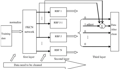
Similarity and smoothness are the two important char-acteristics of electrical load curves. The several peak times in a daily curve are generally the same, and the neighboring points usually have little variation, while the existence of dirty data will obviously destroy the smoothness. However, the similarity remains unchanged because the amount of dirty data is small. Therefore, characteristic patterns can be extracted from many load curves that may contain dirty data using the clustering algorithm of data mining theory, and then, the characteristic curve can be separated from the load curves by a classiﬁcation algorithm and the dirty data will ﬁnally be recognized. The structure of the model is shown inFig. 1.

The ﬁrst layer is a kind of improved Kohonen network (FKCN – fuzzy Kohonen clustering network). The under checked curvexjis the input of the FKCN. If the character-istic curve corresponding to a nerve cell has the biggest sim-ilarity to xj, the nerve cell will output 1 and excite the

corresponding RBF sub-network. The second layer is a RBF sub-network related to each clustering center. After being trained, it is ready to identify the dirty date and locate them accurately. If the output cell of the RBF is close or equal to 1, the corresponding input cell stands for dirty data. The third layer adjusts the dirty data. The detailed principles in term of model layers are described as follows. 2.1. Load data clustering (the ﬁrst layer)

Data clustering is used for extracting the characteristic curve from the load. Clustering algorithms attempt to assess the interaction among patterns by organizing the patterns into clusters so that patterns within a cluster are more similar to each other than those patterns belonging to diﬀerent clusters.

Neural networks, such as the Kohonen clustering net-works (KCNs) have been successfully applied in the area of pattern recognition and clustering [11–14]. One of the advantages of this approach is that it does not need any prior knowledge of the number of clusters present in the data set. However, KCNs suffer from several major prob-lems[15]. Firstly, KCNs are heuristic procedures, so termi-nation is not based on optimizing any model of the process or its data. Secondly, the final weight vectors usually depend on the input sequence. Thirdly, different initial con-ditions usually yield different results. Fourthly, several parameters of the KCN algorithms, such as the learning rate, the size of update neighborhood and the strategy to alter these two parameters during learning must be varied from one data set to another to achieve ‘‘useful’’ results.

A fuzzy Kohonen clustering network (FKCN) model has been proposed by Bezdek in Ref. [15]. This method can overcome some of the diﬃculties described above by taking advantage of the best features of the self organizing structure of the KCNs and the fuzzy clustering model of the FCM. In this paper, the FKCN algorithm has been employed in clustering the load data.

0

Second layer first layer

Data need to be cleaned

Σ 1 adjust 0 normalize Training date FKCN network RBF 1 RBF J-1 RBF J RBF N Data After clean Third layer

(3)

2.1.1. Kohonen clustering networks (KCNs)

The Kohonen model is a neural network that simulates the hypothesized self organization process carried out in the human brain when some input data are presented

[11]. The structure of this neural network is composed of two layers: an input layer formed by a set of units (on for each feature of the input) and an output layer formed by units or neurons arranged in a two-dimensional grid. Each neuron has a vector of coefficients associated with it. It can be interpreted as ‘‘weights’’ attached to the edges that connect the p input nodes to the c output nodes. The aggregate of the c weight vectors (the network weight vec-tor vi) is adjusted during learning. Given an input vector, the neurons in the output layer compete among themselves and the winner (whose weight has the minimum distance from the input) updates its weights and some set of pre-defined neighbors. The process continues until the weight vectors stabilize. In this method, a learning rate must be defined that decreases with time in order to force termina-tion. The updated neighborhood must be defined and is also reduced with time. The KN algorithm process can be seen in Ref.[11].

2.1.2. Fuzzy c-means algorithms (FCM)

Fuzzy c-means clustering [16–18]is a process of group-ing similar objects into the same class, but the resultgroup-ing partition is fuzzy, which means that the patterns are not assigned exclusively to a single class, but partially to all classes. The goal is to optimize the clustering criteria in order to achieve a high intra-cluster similarity and a low inter-cluster similarity usingp-dimensional feature vectors. The theoretical basis of these methods will only be brieﬂy reviewed here.

LetX= {x1,x2,. . .,xn} denote a data set where each

ele-ment inX is a vector withP dimension, the data set Xis going to be partitioned into c fuzzy clusters. A c-partition of X can be represented by uik, where uik is a continuous function in the [0, 1] interval and represents the member-ship ofxkin the clusteri, 16_i6 _c_{, 1}6_k6_n_{. In general}

[uik] can be denoted by ac·nmatrixUand satisﬁes the fol-lowing conditions:

Xc i¼1

uik¼1 ð1Þ

The fuzzy c-means algorithm consists of an iterative opti-mization of an objective function:

JmðU;vÞ ¼ Xn k¼1 Xc i¼1 ðuikÞ m Dik _ð₂_Þ

where the parameterm2(1,1) determines the ‘‘fuzziness’’ of the partition. In this paper, m= 2.0.vi= {v1,v2,. . .,vc}, withviis the cluster center of classi, and

Dik¼ ðdikÞ

2

¼ kxkvik

2

A ð3Þ

is the distance in theAnorm fromxktovi(Ais any positive deﬁnitep·p matrix).

For a given partition, the cluster centers can be calcu-lated as follows: vi¼ Pn k¼1ðuikÞ m xk Pn k¼1ðuikÞm ð4Þ A new partition is obtained as

uik¼ Xc j¼1 ðdik=djkÞ 2 m1 " #1 ð5Þ The iterative optimization of the objective function contin-ues until a stopping criterion is met, usually when the dis-tance between U matrices at successive iterations falls below a threshold, that is

Et¼ kUtUt1k<e ð6Þ FCM is a gradual optimal process with slow convergence. 2.1.3. FKCN

The fuzzy Kohonen clustering network [15]is a type of neural network that combines both methods described above: KCNs and FCM. The structure of this self organi-zation network model consists of two layers: input and out-put. The input layer is composed ofnnodes, wherenis the number of features, while the output layer is formed byc nodes, wherecis the number of clusters to be found. Every single input node is fully connected to all output nodes with an adjustable weightviassigned to each connection. Given an input vector, the neurons in the output layer update their weights based on a pre-deﬁned learning ratea. This approach integrates the fuzzy membership uik from the FCM in the following update rule:

vi;t¼vi;t1þaik;tðxkvi;t1Þ ð7Þ where the learning rateais deﬁned as:

aik;t¼ ðuik;tÞ

mt _ð

8Þ mt¼m0 ðm01Þt=T ð9Þ

m0is any positive constant greater than one,tis the current iteration andTis the iteration limit.

The steps for the algorithm are:

Step 1: Fixc, andeto any small positive constant. Step 2: Initialize the weight vector (cluster centers)

v0= {v1,0,v2,0,. . .,vc,0}. Choose m0> 1 and

maxi-mal iterative stepsT. Step 3: Fort= 1, 2,. . .,T

(a) Compute all learning ratesaikas deﬁned in Eq.

(8).

(b) Update all weight vectorsvi,twith: vi;t¼vi;t1þ Pn k¼1aik;tðxkvi;t1Þ Pn s¼1ais;t ð10Þ (c) ComputeEtfor the stopping criterion, IfEt<e

(4)

2.1.4. Dynamic soft clustering by using SFKN

The sample data is a time sequence and should be updated dynamically with elapsing time. Thus, dirty data adjustment is also a dynamic process. In this paper, a detective threshold value u0 is introduced, and the algo-rithm is detailed as follows:

Step 1: Initializing the dynamic detective threshold value u0.

Step 2: Introducing xþ

j andxj, where xþj means the new

added sample data in the data set andx j stands

for the eliminated sample data. The current sample data can be expressed as: X ¼ ffxjg

þfxþ

jg fxjgg.

Step 3: Calculating uiðjj_Þ, the membership grade of the

remaining dataxjxj towards the clustering

cen-ter vector vi. Setting u

iðjj_Þ¼maxfu_iðjj_Þg, if

u

iðjj_Þ<u0, then eliminating vi, updating

c=c1, and setting all the weights to 0 whose related nodes connect with this node in the FKCN; ifu

iðjj_ÞPu0, remainvi.

Step 4: Calculatinguijþ, whereu_ijþ means the membership

grade of xþ_j toward each clustering center vi. Set u

ijþ ¼maxfuijþg, if u

ijþ <u0, continue the next

step 5; ifu

ijþPu0and then algorithm ﬁnishes. Step 5: Introduce new added clustering centerviþ with

ini-tial valuexþj, setc=c+ 1 and keep other

cluster-ing center unchanged, then choosexþj as the input

of FKCN and calculate new clustering center according to the FKCN algorithm.

In step 5, most of the clustering centers remain unchanged in spite of the little variation with the network structure. At the same time, the membership grade of the original data toward these cluster centers also remains unchanged, so the parameters of the original network can be used in the new network, which will converge quickly.

2.2. Pattern classifying of dirty data (the second layer) In the second layer of the model, the RBF is used to con-struct a pattern classiﬁer for dirty data because of its strong ability of fast convergence and classiﬁcation.

2.2.1. Radial basis function network

The radial basis function (RBF) network[18–21], which is a three layer neural network including input, hidden and output layers. The input layer connections are not weighted, and thus, each hidden node receives each input value, without alteration. The hidden nodes are the radial basis function units. The transfer function for the hidden nodes is non-monotonic in contrast to the monotonic sig-moid function of back propagation networks. The output nodes are simple summations.

The transfer function of the hidden layer in the RBF network often uses a Gaussian function

ai¼expðkX vik=r2iÞ ð11Þ

whereaiis the activation of theith node in the hidden layer, X2Rnis an input vector, vi is called the center vector of the ith node, ri is called the bandwidth vector of theith node, and kkdenotes the Euclidean norm.

The output of the networkyjis given by: y_j¼X

m

i¼1

wjiai ð12Þ

wherewjiis the connected weight between the hidden layer and the output layer, m denotes the number of nodes in the hidden layer.

2.2.2. The dirty data locating algorithm

Each clustering center from the FKCN corresponds to a RBFNN, and the value of the clustering center is selected as the center of Gaussian function of each RBF. Each RBF’s input layer has 96 nodes (corresponds to the 96 load points per day), and the output layer also has 96 nodes, Suppose that only a single dirty data is present and the rest of the data are normal, then choose the sampling number as 96, and then, the pattern number of the dirty data is 96·2 = 192. Input and output sample data sets can be cre-ated as follows:

Step 1: Choosing clustering center vi as the i-th input of the RBFNN, that is, x0=vi, and the correspond-ing output isy0= (0, 0,. . ., 0).

Step 2: Giving the ﬁrst element of vi a deviation, x1= (vi(1) +e,vi(2),. . .,vi(p)), there is products a sample containing dirty data, and output y1= (1, 0,. . ., 0) after; Giving the second element of vi a deviation, x1= (vi(1),vi(2) +e,. . .,vi(p)), there is produced a sample containing dirty data, then outputy1= (0,1,. . ., 0); Continue this opera-tion to the remaining elements of vi and obtain a sample data set with positive deviation.

Step 3: Change the deviation etoeand replace 1 in the output vector by1. Repeat step 2 and obtain a sample data set with negative deviation.

The trained network can identify and locate dirty data accurately no matter how the dirty data exists in the curve: whether there is only a single dirty element or a series. 2.3. Recognition and adjustment of dirty data (the third layer)

The amendment of dirty data is realized in the third layer. The value of the dirty data positioned in the second layer is adjusted by replacing it by the weighted sum of the corresponding two values in the same position in two char-acteristic curves with maximal membership grade. If the sub maximal membership grade is less than 0.2, then the

(5)

value of the characteristic curve with maximal membership grade is chosen. For example, dirty data exists in the curve xjfrom point t1 to t2, andvi1,vi2are two clustering centers with maximal membership grade, then the amendment of the dirty data can be expressed as:

x0_jðtÞ ¼v0_i₁ðtÞ ui1;j ui1;jþui2;j þv0_i₂ðtÞ ui2;j ui1;jþui2;j ð13Þ v0_i₁ðtÞ ¼vi1ðtÞ xjðt11Þ vi1ðt11Þ þxjðt2þ1Þ vi1ðt2þ1Þ =2 ð14Þ v0_i₂ðtÞ ¼vi2ðtÞ xjðt11Þ vi2ðt11Þ þxjðt2þ1Þ vi2ðt2þ1Þ =2 ð15Þ wheret2[t1,t2].

3. The analysis of results

Data in workday and weekend are put into the FKCN, respectively, because these two kinds of load curves are obviously diﬀerent. This operation reduces the amount of training calculation and the number of clustering centers and increases the calculation speed and improves the eﬃ-ciency of the model. The following example is derived from electrical load data from April to September 2003 of the Jiangbei power supply bureau in Chongqing, China. 3.1. Normalization of load data

Similarity and smoothness of curves are mainly consid-ered in this system. As varied amplitude of curves inﬂu-ences the similarity of the curves, in order to eliminate this inﬂuence, we normalize the load as follows:

x0_LðiÞ ¼_P₉₆xLðiÞ

i¼1xLðiÞ

ð16Þ

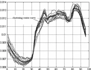
3.2. Training results

The clustering center and curves after normalization are shown inFig. 2.

3.3. Adjusting results

Load data in October 2003 (out of the training set) are adjusted randomly.Fig. 3is a typical load curve with dirty data, where the amendment methods and corresponding results are presented clearly.

3.4. Comparison of accuracy between FKCN and KCNs In order to illustrate the advantages of the FKCN employed in this paper, we replace the FKCN in the first layer of the model by the general Kohonen network. On the basis of daily load data in October 2003, some dirty data are added artificially. The results of the two methods are shown inTable 1where one can find that the accuracy

of the proposed method is higher than that of the KCNs method.

3.5. Dynamic updating algorithm

In order to verify the efficiency of this algorithm, dirty data of 5 days in December 2003 are firstly adjusted with-out using the dynamic updating algorithm (sample data is from April to September in 2003). Then, the model of the dynamic updating algorithm is used, and the sample data set is updated till the day before the identification day. Results are shown inTable 2.

The results of the dynamic updating algorithm are satis-fying because its error is less than that of the non-dynamic algorithm. In the dynamic updating algorithm, the latest adjusted clustering center and vectors are used, which increases the membership grade of the load curves and clustering centers. However, the dynamic updating algo-Fig. 2. Normalized curves and clustering center of one type of loads.

Fig. 3. Identiﬁcation of dirty data. 1: load curve; 2: clustering center with maximal membership grade 3: clustering center with sub-maximal membership grade; 4: curve after adjusted.

(6)

rithm improves not only the accuracy of identiﬁcation but also the adjustment precision of the dirty data.

4. Conclusion

The analysis of examples illuminates that the FKCN algorithm improves the capability of Kohonen clustering networks and can obtain the clustering center more quickly and reasonably, overcoming the disadvantages of the Kohonen algorithm. The proposed dynamic updat-ing algorithm can adjust the clusterupdat-ing center automati-cally on the basis of the newly added data, and the RBF networks can identify the exact location of dirty data because of its strong ability of pattern recognition. The dynamic intelligent adjusting model proposed in this paper can process data dynamically with higher accuracy and faster convergence.

References

[1] Rahman S, Bhatnagar R. An expert system based algorithm for short term load forecast. IEEE Trans Power Syst 1988;3(2):392–9. [2] Mori H, Kobayashi H. Optimal fuzzy inference for short-term load

forecasting. IEEE Trans Power Syst 1996;11(1):390–6.

[3] Song Kyung-Bin, Baek Young-Sik, Hun Hong Dug, Jang Gilsoo. Short-term load forecasting for the holidays using fuzzy linear regression method. IEEE Trans Power Syst 2005;20(1):96–101. [4] Kim KH. Development of fuzzy expert system for short-term load

forecasting on special days. IEEE Trans Power Syst 1998;47(7):886–91.

[5] Nazarko J, Zalewski W. The fuzzy regression approach to peak load estimation in power distribution systems. IEEE Trans Power Syst 1999;4:809–14.

[6] Charytoniuk W, Chen M-S. Very short-term load forecasting using artiﬁcial neural networks. IEEE Trans Power Syst 2000;15(1):263–8. [7] Ling SH, Frank HF Leung, Lam HK, et al. Short-term electric load forecasting based on a neural fuzzy network. IEEE Trans Ind Electron 2003;50(6).

[8] Fayyad UM et al., editorsAdvances in knowledge discovery and data mining. AAAI Press/MIT Press; 1996.

[9] Cho Kokyo. Outlier detection for stationary time series. J Stat Plan Infer 2001:111–27.

[10] Nicolaos B Karayiannis. An axiomaticn approach to soft learning vector quantization and clustering. IEEE Trans Neural Networks 1999;10(5):1015–9.

[11] Kohonen T. Self-organization and associative memory. 3rd ed. Ber-lin: Springer; 1989.

[12] Huntsberger T, Ajjimarangsee P. Parallel self-organization feature maps for unsupervised pattern recognition. Int J Gen Syst 1989:357–72.

[13] Hartigan J. Clustering algorithms. New York: Wiley; 1975. [14] Dubes R, Jain A. Algorithms that cluster data. Englewood

Cliﬀs: Prentice Hall; 1988.

[15] Tsao EC, Bezdek JC. Fuzzy Kohonen clustering networks. Pattern Recogn 1994;27(5):757–64.

[16] Dubois D, Prade H. Fuzzy sets and system: theory and applica-tions. New York: Academic Press; 1980.

[17] Bezdek JC. Pattern recognition with fuzzy objective function algo-rithms. New York: Plenum Press; 1984.

[18] Broomhead DS, Lowe D. Multivariable functional interpolation and adaptive networks. Complex Syst 1988;2:321–55.

[19] Moody TJ, Darken CJ. Fast learning in networks of locally tuned processing units. Neural Comput 1989;1:151–60.

[20] Bishop CM. Neural networks for pattern recognition. Oxford: Clar-endon Press; 1995. p. 164–91.

[21] Chen S, Cowan CFN, Grant PM. Orthogonal least squares learning algorithm for radial basis function networks. IEEE Trans Neural Networks 1991;2:302–9.

Table 1

Comparison of two amendment models Dirty data

points

Error before adjust (%) General Kohonen (%) SFKN (%) 1 26.4 4.7 2.8 2 32.3 7 3.3 3 15.5 4.2 2.1 4 17.6 3.8 2.4 5 8.5 5.6 1.9 Table 2

The result of random check to load data Date no. Count of dirty data Non-dynamic algorithm Dynamic updating algorithm Failed to judge Misjudged Failed to judge Misjudged 1 20 3 2 1 1 2 15 5 2 1 0 3 18 2 0 0 0 4 17 1 2 1 0 5 20 3 1 0 2 Total 90 14 7 3 3