Inaugural-Dissertation
zur Erlangung des Grades eines Doktors der Wirtschafts- und Gesellschaftswissenschaften
durch die
Rechts- und Staatswissenschaftliche Fakult¨at der Rheinischen Friedrich-Wilhelms-Universit¨at
Bonn
vorgelegt von Sinem Hacıo˘glu Hoke
aus Ankara (T¨urkei)
Erstreferent: Prof. Dr. Matei Demetrescu
Zweitreferent: Prof. Dr. Christian Pigorsch
This dissertation would not have been completed without the help and the support of many people. First and foremost, I would like to express my gratitude to my supervisor Matei Deme-trescu who has stood by me since my first day. His sincere comments and endless help enabled me to come this far. He was always more than a supervisor for me. I appreciate what he taught me as a professor and a mentor.
I would like to thank my second advisor Christian Pigorsch for believing in me and agreeing to supervise my second paper even though I was abroad. I am very grateful to find the opportunity of having him in my committee. Many thanks to Benjamin Born for being the third member of my thesis committee.
I am thankful to be given the opportunity to be a part of Bonn Graduate School of Economics. I would also like to thank the German Research Foundation (DFG) for financial support in this respect. I was very privileged to go to University of Wisconsin-Madison for a year during my studies. I could not have done it without the aid of and the financial support through the International Office. I greatly benefitted from the fruitful comments of Jack Porter.
Many thanks go to my dear friend and my coauthor Kerem Tuzcuoglu for supporting me, helping me a great deal and even covering my lack of proceeding on certain concepts. I know that he will be a great academic one day and more people will benefit from his sight. I will be there to give him a big applause.
I would like to thank Jeremy Chiu to support me during my internship at the Bank of England. His support made it possible me to come where I am now. I will be always most thankful to
your help on the third chapter of this thesis. Moreover, I am very lucky to have the opportunity to work with Tomasz Wieladek during the internship.
Life would have been really difficult without my friends in Bonn. I established life time friend-ships here. I am indebted to Buket and Demet for sharing both my problems and my joy with me in the last 6 years. They always believed in me, looked out for me and opened their priceless hearts to me. You will be present in every single stage of my life.
My fellow grad friends, Andreas Kleiner, Anke Becker, Benjamin Enke, D´esir´ee R¨uckert, Lien Pham-Dao, Moritz Drexl, Ralph L¨utticke created a great atmosphere despite the hard processes we had been all going through. Living in a different country and trying to get used to a new life along with professional obligations were simplified by your existence in my life. I will definitely miss watching soccer, having beer and chatting with you. I am very lucky to have you all. I am looking forward to dancing at more weddings! And I am very lucky to be the aunt of Ben and Anke’s daughter, the cutest Leni ever!
Most importantly, special thanks to my family who supported me along this long path. Mom, you have been always there for me even through Skype. You always made me feel that I have a safe place to be. Gizem, you are the best sister ever and I still have no idea how you are always able to cheer me up! Dad, I know you are there somewhere watching me.
Lastly, I would like to thank my Justin for showing up in my life unexpectedly, very surprisingly but exultantly. I will always appreciate the circumstances which lead me your way. I could not have survived the last three years without the thought of our amazing future. I know you will be always there for me.
Sinem Hacioglu Hoke London
Motivated by the recent availability of extensive macroeconomic data sets, this thesis consists of three independent chapters that examine the ways to approach to this issue from various angles. CHAPTER 1. The first chapter, which is a joint work with Matei Demetrescu, discusses the particularities of forecasting with factor-augmented predictive regressions under general loss functions. In line with the literature, principal component analysis is employed to extract factors from the set of predictors. We also extract information on the volatility of the series to be predicted, since volatility is forecast-relevant under non-quadratic loss functions. Moreover, the predictive regression is estimated by minimizing the in-sample average loss, to ensure asymptotic unbiasedness of forecasts under the relevant loss. Finally, to select the most promising predictors for the series to be forecast, we employ an information criterion tailored to the relevant loss. Using the Stock and Watson data set, we assess the proposed adjustments in a pseudo out-of-sample forecasting exercise. Expectedly, the use of estimation under the relevant loss is found to be effective. In other words, the forecasting exercises we employ suggest that evaluating forecasts under the chosen asymmetric loss function lead to smaller forecast losses. Using an additional volatility proxy as predictor and conducting model selection tailored to the relevant loss function further enhance forecasts. Both the theoretical and the empirical results emphasize the importance of using the relevant loss functions while performing forecasting exercises with extracted factors.
CHAPTER 2. The second chapter is a joint paper with Kerem Tuzcuoglu and is linked to the first chapter in the factor analysis sense. Researches have not found a way to assign economic meaning to factors although factor analysis has been widely used as a dimension reduction method. In this paper, we propose a Threshold Factor Augmented Vector Autoregression model
to address this issue. The novelty is the interpretation of factors by observing how frequently factor loadings fall below estimated thresholds and become irrelevant. The results indicate that we are able to relate most of the factors to specific categories of the data without any prior specification on the data set. Furthermore, the interpretable factors, e.g., real activity factor, unemployment factor and such, are each given shocks along with policy shock to observe the responses of the other factors and individual series. The resulting impulse responses are of expected sign and magnitude in general. Overall, our results yield an intensive layout on which factor is associated with different aspects of the economy. We are able to associate the extracted factors with certain macroeconomic activities, such as real economy, unemployment, inflation. We present impulse response analysis to show how a contractionary monetary shock affects the factors and variables. Our results are consistent with what the economic theory suggests. CHAPTER 3. The third chapter, written in collaborative work with Jeremy Chiu, uses the large information sets in vector autoregression sense. Motivated by the desire to probe macroeco-nomic tail events and to capture nonlinear ecomacroeco-nomic dynamics, we estimate two types of regime switching models with Bayesian estimation methods: Threshold VAR and Markov switching VAR. We also use linear Bayesian VAR model as a benchmark. For each of the non-linear mod-els, we estimate regimes which carry the interpretation of recessionary/normal and financially stressful/stable periods. Using the recursiveness assumption and conditional on shocks of one-standard-deviation, we show that (i) financial shocks hitting during times of recessions create disproportionately more severe contractions in output; (ii)output growth shocks hitting in finan-cially stressful times result in disproportionately further financial stress. We also demonstrate the power of a feedback loop between real and financial sectors when extremely large shocks hit the economy in normal/financially stable periods. Afterwards, we perform out-of-sample forecasting exercises, and find that the Threshold VAR model has the potential to predict tail events in conditional forecasting compared to the Markov switching VAR and Bayesian VAR. Our findings provide strong evidence of nonlinearities and shock amplification mechanisms in the United Kingdom data, and hence useful information to investigate macroeconomic tail events.
Introduction . . . iii
1 Macroeconomic Forecasting with Large Data Sets under Asymmetric Loss 1 1.1 Motivation . . . 1
1.2 The basic forecasting problem . . . 4
1.3 Extracting additional relevant information . . . 7
1.4 Forecasting under asymmetric loss . . . 11
1.4.1 Setup . . . 11
1.4.2 Extracted factors . . . 12
1.4.3 Results . . . 15
1.5 Concluding remarks . . . 18
Appendix 1 20 1.A An information criterion . . . 20
1.B Proof of Proposition 1 . . . 20
1.C Model selection using the LASSO . . . 23
2 Interpreting Latent Dynamic Factors by Threshold FAVAR Model 33
2.1 Introduction . . . 33
2.2 The Model . . . 36
2.2.1 Model Specification . . . 36
2.2.2 Bayesian Estimation . . . 38
2.2.3 Identification Restrictions for Factors . . . 39
2.3 The Data . . . 40
2.4 Results . . . 41
2.4.1 Number of Factors in the Data . . . 41
2.4.2 Interpreting the Factors . . . 42
2.5 Impulse Response Functions . . . 45
2.6 Concluding Remarks . . . 48
Appendix 2 51 2.A Priors and Posteriors . . . 51
2.A.1 Priors . . . 51
2.A.2 MCMC Estimation Steps . . . 51
2.B Different Restrictions onΛt . . . 56
2.C Impulse response functions . . . 57
2.D Data Description For SW Updated Data . . . 60
3 Macroeconomic Tail Events with Non-linear BVARs 64 3.1 Introduction . . . 64
3.2 Model Specifications . . . 68
3.2.2 Markov Switching Vector Autoregression Models . . . 70
3.2.3 Benchmark Bayesian VAR . . . 70
3.3 Data . . . 70
3.4 Full sample estimation results . . . 71
3.5 Impulse Response Analysis of Structural Shocks . . . 73
3.5.1 Generalised impulse response functions and shock identification . . . 74
3.5.2 Shock propagation and macro tail events . . . 75
3.5.3 Tail shocks and the feedback loop . . . 78
3.6 Forecasting analysis . . . 79
3.7 Concluding remarks . . . 80
Appendix 3 90 3.A Normal Inverse Wishart priors . . . 90
3.B The Gibbs Sampling algorithm for TVAR . . . 91
3.C The Gibbs Sampling algorithm for MSVAR . . . 91
3.C.1 An extension: MSVAR with two independent Markov chains . . . 93
3.D Generalized Impulse Response Functions . . . 95
3.D.1 GIRFs for TVAR . . . 95
3.D.2 GIRFs for MSVAR . . . 96
3.E Variables . . . 96
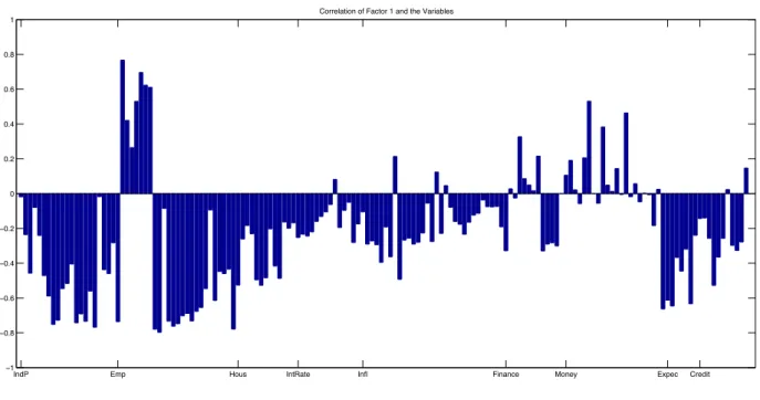
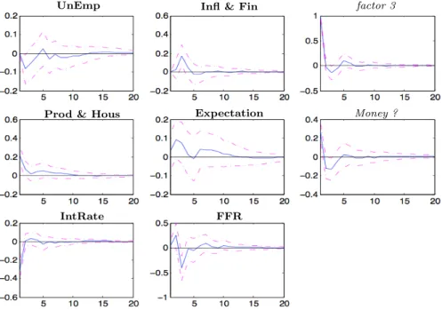
2.1 The correlation between the variables and the first factor . . . 44 2.2 The responses of the factors and FFR to a 1 unit shock on FFR. . . 46 2.3 The responses of the factors and FFR to a 1 unit shock on unemployment factor. 47 2.4 The responses of the variables to a 1 unit shock onFFR. . . 47 2.5 The responses of the factors and FFR to a 1 unit shock oninflation and finance
factor. . . 57 2.6 The responses of the factors and FFR to a 1 unit shock onthird factor. . . 57 2.7 The responses of the factors and FFR to a 1 unit shock onreal activity factor. . 58 2.8 The responses of the factors and FFR to a 1 unit shock onexpectations factor. . 58 2.9 The responses of the factors and FFR to a 1 unit shock onmoney factor. . . 59 2.10 The responses of the factors and FFR to a 1 unit shock oninterest rate factor. . 59
3.1 Full sample regimes for TVAR-Y . . . 72 3.2 Full sample regimes for TVAR-S . . . 73 3.3 Full sample regime probabilities for MSVAR . . . 74
3.4 Impulse Responses to a 1 SD adverse shock to corporate bond spreads in BVAR model . . . 82 3.5 Generalised Impulse Responses to a 1 SD adverse shock to corporate bond spreads
in TVAR-Y model . . . 82 3.6 Generalised Impulse Responses to a 1 SD adverse shock to corporate bond spreads
in TVAR-S model . . . 83 3.7 Generalised Impulse Responses to a 1 SD adverse shock to corporate bond spreads
in MSVAR model . . . 83 3.8 Impulse Responses to a 1 SD adverse shock to real GDP growth in BVAR model 84 3.9 Generalised Impulse Responses to a 1 SD adverse shock to real GDP growth in
TVAR-Y model . . . 84 3.10 Generalised Impulse Responses to a 1 SD adverse shock to real GDP growth in
TVAR-S model . . . 85 3.11 Generalised Impulse Responses to a 1 SD adverse shock to real GDP growth in
MSVAR model . . . 85 3.12 Impulse Responses to a 1 SD adverse shock to short term interest rate in BVAR
model . . . 86 3.13 Generalised Impulse Responses to a 1 SD adverse shock to short term interest
rate in TVAR-Y model . . . 86 3.14 Generalised Impulse Responses to a3 SD adverse shock to real GDP growth
in TVAR-Y model (to be compared with Figure 3.9) . . . 87 3.15 Generalised Impulse Responses to a3 SD adverse shock to corporate bond
spreads in TVAR-S model (to be compared with Figure 3.6) . . . 87
3.16 Unconditional predictive densities for the three models . . . 88 3.17 Conditional predictive densities based on the path of Corporate Bond Spreads . . 89 3.1 Full sample regimes for MSVAR with 2 independent Markov chains . . . 94 3.2 Variables . . . 98
1.1 Factors selected for predicting for all predictor series by AICL; full data span . . 14
1.2 Losses Evaluated for OLS-Asymmetric Loss and Asymmetric Loss . . . 16
1.3 Tests of equal predictive accuracy of OLS and AL based forecasts . . . 17
1.4 Selection of Factors (LASSO), full data span . . . 25
1.5 Average Losses with LASSO-based model selection - Parsimonious post-fit LASSO 27 1.6 Average Losses with LASSO-based model selection - Flexible post-fit LASSO . . 28
2.1 Subgroups in the Data Set . . . 41
2.2 Number of Factors for Different Time Spans . . . 42
2.3 Survival Rates of the Factor Loadings . . . 43
2.4 Survival Rates of the Factor Loadings under Different Restrictions . . . 56
3.1 Summary statistics . . . 97
1
Macroeconomic Forecasting with Large Data Sets under Asymmetric Loss
1.1
Motivation
In forecasting macroeconomic series, the past decade has witnessed the increased availability and use of comprehensive data sets consisting of a large number of predictor time series. When forecasting macroeconomic aggregates like inflation or GDP, the appeal of such auxiliary data-rich sets is understandable: the additional informational content of the series helps improving forecasts compared to a benchmark (vector) autoregression of the variable to be predicted. At the same time, dealing with an increased number of predictor series poses problems, since the number of time observations is typically comparable with the number of series in such sets. This leads to imprecise coefficient estimates in an augmented predictive autoregression, and consequently to a trade-off between availability and usability of information. The literature has therefore focussed on complexity reduction and information extraction. Factor-based forecasting models, for which it is assumed that unobserved common components of the auxiliary series are good predictors for the variable of interest, are particularly popular in this respect.
Since the predictors are not observed directly for factor-based forecasts, the forecasting procedure boils down to estimating a feasible predictive regression using lags of the dependent variable and
extracted factors as right-hand side variables. Several contributions have shown that a relatively small number of estimated factors successfully summarize the contemporaneous information in
the data set of predictors. Stock and Watson(2002c) demonstrate Principal Component Analy-sis [PCA] of the predictors to produce conAnaly-sistent estimates of the space spanned by the common factors. Their factor model forecasts outperforms other benchmark models to forecast personal income and output growth; see also the earlier work inStock and Watson (1998). Focussing on estimation and inference in approximate factor models,Bai (2003) derives asymptotic distribu-tions and uniform convergence results while Bai and Ng(2002) provide information criteria for estimating the number of factors; see alsoAlessi et al. (2010).
The popularity of factor models in forecasting is reflected by the large number of contributions in the applied literature. Ludvigson and Ng(2009a,c) use factors from a large number of macroe-conomic series to predict excess bond returns and to show that the predictability of future excess returns is related to macroeconomic activity. These are just the tip of the iceberg; seeMarcellino et al. (2003), Artis et al. (2005), den Reijer (2005), Forni et al. (2005), Banerjee et al. (2008),
Engel et al.(2012) orGodbout and Lombardi(2012) to name but a few more contributions to the literature on factor-based forecasting. While there are alternative approaches such as soft/hard thresholding or forecast combinations, they appear to be less popular than factor-based models. One reason to prefer factor-based forecasting procedures may be their interpretability; see e.g. the discussion inLudvigson and Ng (2009a,c). For instance, Ludvigson and Ng (2009c) regress each macroeconomic variable in their data set on the PCA-extracted factors. TheR2s of these regressions are informative of the relations between the factors and the variables. They are thus able to identify e.g. stock market, inflation or real factors. More recently, Hacioglu Hoke and Tuzcuoglu(2014) work on factor augmented VAR models with a threshold structure of the loadings (which are dynamic in their setup). The periods where the loadings are set to zero or where the factors load more heavily on the variables are also informative on the relations between factors and variables. The point is that predictors with economic meaning prevent the interpretation of forecasting procedures as “crystal-ball” or “black-box” econometrics and are more likely to produce forecasts understandable by wider audiences.
The focus of the work cited above is on forecasts which are optimal in the mean squared-error [MSE] sense, i.e. on procedures minimizing the expected squared forecast error. The literature documents, however, a significant number of cases where more general – and in particular asym-metric – cost-of-error functions are employed. For instance, IMF and OECD forecasts of the deficit of G7 countries are found by Artis and Marcellino (2001) to be systematically biased towards over or under-prediction when compared with MSE-optimal forecasts. Elliott et al.
(2005b) propose formal methods of inference on the degree of asymmetry of the loss function and testing the rationality of forecasts; see also Patton and Timmermann (2007b). Building on the work of Elliott et al., Christodoulakis and Mamatzakis (2008, 2009) find asymmetric preferences of EU institutional forecasts. Clements et al.(2007) discuss the loss function of the Federal Reserve and Capistr´an (2008) even finds that, for inflation, the forecasting preferences of the Fed are time-varying. The loss function of the Bank of Canada is analyzed by Pierdzioch
et al. (2011). More recently, Tsuchiya (2016) examines the asymmetry of the loss functions of the Japanese government, the IMF and private forecasters for Japanese growth and inflation forecasts.
We therefore study factor-augmented forecasting under asymmetric loss. For a given predictive model, there is little debate as to how to obtain point forecasts under a given loss function: it has been known since Weiss and Andersen(1984) and Weiss (1996) that the forecast model should be estimated under the relevant loss.1 Estimation of the feasible predictive regression under the relevant loss would therefore improve forecasts. This prompts the question, first, whether such estimation may indeed be conducted with estimated factors in a manner analogous to the MSE-optimal case. Less obvious however, is the second question of whether the forecast model should be the same under any asymmetric loss function. To put it bluntly, are the PCA-extracted factors still forecast-relevant under an asymmetric loss function? Considering the theory of forecasting under asymmetric loss functions, see Granger(1969),Granger (1999),Weiss(1996),
Christoffersen and Diebold(1996),McCullough(2000),Elliott and Timmermann(2004),Elliott et al.(2005b),Patton and Timmermann(2007a) orPatton and Timmermann(2007b), the least what may be expected is that the relative importance, as a predictor changes, for the extracted factors or even for the lags of the dependent variable in the augmented predictive autoregression. So, rather than relying on the summarizing power of, say, the first principal component, one may have to select the predictors (lagged dependent variables or factors) that are most informative under the relevant loss.2 Third, perhaps even more importantly, one should ask whether the usual factor extraction does actually capture all information relevant under the given loss function. PCA essentially delivers linear combinations of the “many predictors” data set. In a linear predictive model under squared-error loss, this may be a convenient dimensionality reduction procedure. But the optimal forecast function under an asymmetric loss function may depend on the auxiliary series in a non-linear fashion, even if the optimal forecast function is linear in the MSE-optimal case. Thus, the informational content of the data set may not be fully exploited under an asymmetric loss function.
Our contributions are as follows. We show in Section 1.2 that, regularity conditions provided, one may indeed use PCA-extracted factors as predictors even when estimating forecast regressions using the relevant loss function. To make sure that relevant information is not wasted, we make use in Section 1.3 of the insight that the optimal point forecast under a general loss depends on the conditional variance of the variable to be predicted (Christoffersen and Diebold, 1996;
Patton and Timmermann, 2007b). Thus, adding information on the volatility of the series to be predicted in the forecasting model improves forecasts under asymmetric loss. While the 1An alternative, more demanding, procedure is to model the entire predictive distribution and derive the point
forecasts based on it; see e.g.McCullough(2000) for an ingenious bootstrap-based version.
2In fact, focussing on extracting the factors with the highest associated eigenvalue might not be a good idea
in the MSE-case either, since a factor even if explaining most of the variance of the raw predictor series, need not capture the information relevant for forecasting.
volatility of interest is not observed directly, it is plausibly related to the variability of the auxiliary series. The relation is not a forced one, since the volatility of the overall economic environment should be reflected – at least to some extent – by the volatility of all series involved. This common component can in turn be extracted from the auxiliary data set. Concretely, we extract additional factors from the log-squared residuals of the factor model to increase the quality of the forecasts under the relevant loss. This delivers a larger number of predictors, of which not all need be equally relevant. To find the ones with the highest predictive power, we resort to a suitable information criteria.3
We then illustrate the proposed procedure in Section 1.4 by means of a forecasting exercise with US personal income, industrial production, unemployment rate and retail sales. We use a data set which has become widely known as the “Stock and Watson” data set (Stock and Watson, 2005). Expanded by Ludvigson and Ng (2009a), the data set spans the period from January 1964 to the end of 2007. Although the original data set includes more time series than we work with here, the use of this particular selection of 131 series has been quite popular in the literature; see e.g. Belviso and Milani (2006), Boivin and Ng (2006), D’Agostino and Giannone(2006),Ludvigson and Ng(2009a,c) andBai and Ng(2011). The detailed description and other features of the data can be found in Appendix 1.D. Here, we are interested in one-year-ahead forecasts; working with monthly data, we thus work at forecast horizonh= 12. We compare the average forecast losses of all four variables in every single case we look into. We find, expectedly, that average losses of forecasts produced under the relevant loss function give smaller losses compared to the losses produced by forecasts obtained via OLS estimation of the predictive regression. At the same time, we also show that adding information from the volatility of the series and having parsimonious models by assessing the relevance of the extracted factors improve the average losses.
The final section concludes, and some mathematical details and additional results have been gathered in the Appendix.
1.2
The basic forecasting problem
Letytbe the series for which anh-step ahead forecast is required. Given the available information
set Ft={ft,k, yt, yt−1, . . .}, the optimal forecast is given by
yoptt+h = arg min
y∗ t+h E L yt+h−y∗t+h |Ft , (1.1) 3
The issue of model selection is not restricted to our setup: e.g. Schumacher(2007) compares the forecast accuracy of variety of factor models to MSE-predict German GDP, and finds that results may change when different information criteria to select factors are used.
where L(·) is the relevant loss function quantifying the cost incurred by discrepancies between a given forecast yt∗+h of the variable y at some time t+h and the actual realization yt+h.
According toGranger(1999), loss functions should be uniquely minimized at the origin, and be quasi-convex. We shall work with a specific class of loss functions, introduced by Elliott et al.
(2005b); a forecast y∗t+h is thus evaluated by means of
L yt+h−y∗t+h = α+ (1−2α)I yt+h−yt∗+h <0 yt+h−yt∗+h p . (1.2)
This class of loss functions is quite flexible: it includes as special cases the widely used symmetric (for α = 0.5) and asymmetric (for 0 < α < 0.5 or 0.5 < α < 1); linear and quadratic loss functions (for p = 1 and p = 2). Moreover, it only requires mild moment conditions on yt, in
contrast e.g. to the well-known linex loss. We start with the usual linear forecasting model
yt+h=c+ q X j=1 ajyt−j+1+ r X k=1 bkft,k+vt+h, t= 1,2, . . . , T , (1.3)
where the forecast errorvt+h cannot be predicted under L. This does not imply, however, that
vt+h could not be forecast under another loss function. The lack of predictability ofvt+h underL
implies that the so-called generalised forecast error L0(vt+h)is uncorrelated with the predictors
yt−j+1 andft,k; seeGranger(1999) andPatton and Timmermann(2007a). The optimal forecast
is thus given by ytopt+h=c+ q X j=1 ajyt−j+1+ r X k=1 bkft,k. (1.4)
In practice, one resorts to a two-stage procedure, given that observations onNauxiliary variables
xt,i are available, from which ft,k may be estimated in a first stage. Maintaining the typical
assumption of linear measurement equations for the factors, we have that
xt,i =
r
X
k=1
λi,kft,k+ut,i. (1.5)
With additional conditions on λi,k and ut,i (in particular orthogonality of the common and
idiosyncratic components ft,k and ut,i), extraction of the unknown factors can be conducted,
leading tofˆt,k(we resort to PCA to this end). This ultimately takes us to the feasible predictive
regression yt+h=c+ q X j=1 ajyt−j+1+ r X k=1 bkfˆt,k+vt+h, (1.6)
to be estimated under the relevant loss in a second stage, i.e. ˜ c,˜aj,˜bk= arg min c∗,a∗ j,b∗k 1 T T−h X t=q L yt+h−c∗− q X j=1 a∗jyt−j+1− r X k=1 b∗kfˆt,k , (1.7)
from which the forecast is obtained as
˜ ytopt+h= ˜c+ q X j=1 ˜ ajyt−j+1+ r X k=1 ˜b kfˆt,k. (1.8)
Its quality hinges on the precision of the factor approximation; recall that factors cannot be consistently estimated in a fixed-N setup.
The justification to use the feasible forecast from (1.8) is provided by the following proposition establishing its consistency as T, N → ∞ for the unfeasible optimal forecast from (1.4) under the relevant lossL.
Proposition 1. Let the auxiliary variables xt,i obey Assumptions A-E in Bai (2003). Further-more, assume that the factorsft,kand the forecast errorsvt+h are strictly stationary and ergodic, and that the generalised forecast errors L0(v
t+h) satisfy E (L0(vt+h)|yt, yt−1, . . . , ft,k) = 0 and have no atom at 0. Finally, let all series have finite moments of orderpwithpfrom (1.2)integer and positive. It then holds for the estimated optimal forecast from (1.8)that, point-wise in t,
˜
yoptt+h →p yoptt+h
as N, T → ∞ such thatT /N →0.
Proof: See Appendix 1.B.
Remark 2. Assumptions A-E in Bai (2003) ensure the uniform (in t) consistency of the ex-tracted factors, which, in that framework, may be heteroskedastic and even locally trending. The additionally required strict stationarity simplifies the proofs; while it is slightly more restrictive than the often made assumption of weak stationarity (see e.g. Stock and Watson, 2002c), it is a convenient price to pay for being able to use non-MSE loss functions. Strict stationarity of the factors might be relaxed at the expense of additional conditions, but we do not pursue the topic here as we would rather focus on the forecasting procedure than on more involved technical details. The critical requirement is that the generalised forecast error is a martingale difference sequence, which is a standard condition in the literature on forecasting under asymmetric loss (Patton and Timmermann, 2007a). In a nutshell, the forecast errors must be unforecastable
under the relevant loss. The finiteness of the pth order moments ensures that the forecast risk is finite and an optimal forecast exists.
Remark 3. In factor models, the factors are only identified up to a rotation. But it follows from the proof that rotations do not affect the result: essentially, Pr
k=1˜bkfˆt,k consistently estimates
Pr
k=1bkft,k which is the quantity required for forecasting yt+h. E.g. Bai and Ng(2006) consider this explicitly; to keep notational effort at a minimum, we assume identification directly.
Remark 4. The loss function does not play any role in estimating the factors, but only in the subsequent forecasting step. The main reason to do so is to maintain the interpretability of the factors as economic driving forces (not depending on individual loss preferences), but we also wish to stay in line with the literature on factor-based forecasting. While Tran et al. (2014) discuss estimation of factors under asymmetric linear and asymmetric quadratic losses, these losses refer to the idiosyncratic components and not to the actual forecast errors; we leave the integration of the two approaches to further work.
1.3
Extracting additional relevant information
The two-step procedure for forecasting under asymmetric loss discussed in the previous section is the natural extension of the original method ofStock and Watson(2002c), for which the second step – i.e. estimation of the predictive regression – has been modified to account for the use of a specific loss function. But we should ask at this point whether the first stage – i.e. extracting the information carried by the auxiliary variablesxt,i – is to be left unmodified. In other words,
is the factor model (1.5) exhausting the possibilities of finding predictors for yt+h under the
relevant loss?
It should be pointed out that the linear model (1.5) is only sufficient under conditions which are not plausible for macroeconomic data sets. Namely,Patton and Timmermann(2007b) show that, for loss functions of the type given in (1.2), the optimal forecast has the form
yoptt+h = E (yt+h|yt, yt−1, . . . , xt,i) +C
q
Var (yt+h|yt, yt−1, . . . , xt,i) (1.9)
for some constantC depending on the loss function and the shape of the conditional distribu-tion.4 The first summand on the r.h.s. of (1.9) is nothing else that the conditional mean which the original factor-based model does indeed capture. The coefficient C, and thus the second
summand, is zero e.g. when α = 0.5 and p = 2, or when α = 0.5 and the conditional distri-bution of yt+h is symmetric, but not in general. When estimated under the relevant loss, the
interceptcof the predictive regression (1.3) only captures theaverage of the so-called bias term
CqVar (yt+h|yt, yt−1, . . . , xt,i) and misses the fact that the conditional standard deviation of
yt+h,if time-varying, is actually a predictor foryt+h under L.
And indeed, the volatility of macroeconomic variables is not constant in general. The Great Moderation is the perhaps best known case of time-varying volatility. The term coins the downward trend in the variance of inflation and economic growth since the 1980s (e.g., Stock and Watson, 2002b); Clark(2009) finds that the recent financial crisis has reversed the trend, thus strengthening the evidence of time-varying volatility. Along the same lines, Sensier and van Dijk (2004) find that four out of five of over two hundred U.S. macroeconomic time series exhibit unconditional volatility changes during the period 1959-1999.
What is more, it is expected that such volatility trends are common to the variables in the data set used for forecasting: the series stem, after all, from the same economic environment. Thus, we may resort to the same data set {xt,i} in order forecast the conditional standard deviation
of yt+h.
To exploit the above insight, we assume a stochastic volatility model of the form
vt+h =ete
1 2(gt+
Ps
l=1ξlht,l).
We follow Nelson (1991) in using the exponential “link” function, since it allows us to avoid positivity restrictions on the componentsgt and ht,l and assume – in line with the very idea of
factor-based forecasting – thatht,l could be forecast using information from the auxiliary series
xt,i; gt is an unforecastable component. When the conditional variance of the idiosyncratic
components in the factor model depend in a similar manner on ht,l, we write
ut,i=et,ie
1 2(gt,i+
Ps
l=1ht,lξl,i),
where gt,i are individual volatility components specific for xt,i. As usually, et and et,i are
stan-dardised variables, mutually independent and independent of ht,l,gtand gt,i. Then,
logu2t,i = loge2t,i+gt,i+ s
X
l=1
ξl,iht,l,
which is nothing else than a factor model for the log squares of ut,i with ht,l the common
components and loge2t,i+gt,i the idiosyncratic ones.
Since the variables ut,i are not observed directly, we resort to the idiosyncratic components
second-stage PCA, leading toˆht,l. Note that the factors ft,k themselves may be (conditionally)
heteroskedastic; we assume that they do not bear additional predictive power for the conditional variance of yt+h, but one may of course consider their log squares when extracting ht,l.
This is related to decomposition of the yield spreads in Ludvigson and Ng (2009a,c). In both papers, additional information carried by the yield risk premium (or term premium) is acknowl-edged, due to the inability of the yield curve to explain business cycle variations in bond risk premia. The yield risk premium can be seen as an idiosyncratic error which should be constant under the expectation hypothesis. Ludvigson and Ng estimate this term via the average multi-step estimates of bond returns. They show that the predictive factors are not sufficient to display the countercyclical form of bond risk premia since the predictive power of these factors does not imply explaining the yield curve. In this respect, the additional information used, namely the yield risk premium, parallels the volatility factor we use in this paper.
Equation (1.9) shows that a nonlinear forecast may be better suited in an asymmetric loss context. Clearly, extracting factors from logu2t,i is not the only way to consider nonlinearities; for instance Bai and Ng (2008a) employ quadratic PCA. But Equation (1.9) motivates us to look directly for variables driving the volatility.
Ideally, we would include a term of the form Ce12
Ps
l=1ξlˆht,l in the predictive regression with
additional parametersξl(withgtnot being predictable,e1/2gt is absorbed in the error component
et multiplicatively). But a non-linear regression equation is perhaps too cumbersome to deal
with numerically, even if we must anyway resort to numerical optimization under non-MSE loss.5 We therefore linearize the exponential, ex ≈1 +x, and trade some misspecification in exchange for increased clarity of the final procedure.
The componentgtis in principle not forecastable, at least not fromxt,i, and we treat it as such
by absorbing it in the forecast error. We thus obtain as estimated predictor foryt+h
˜ ytopt+h= ˜c+ q X j=1 ˜ ajyt−j+1+ r X k=1 ˜b kfˆt,k+ s X l=1 ˜ ξlhˆt,l, (1.10)
where the parameter estimates are obtained like before by minimising the observed forecast loss. Due to the linearization, the estimators ξ˜l in (1.10) do not converge to the population values.
The following proposition guarantees that the fitted predictor is the bestlinear predictor under the given loss.
Proposition 5. Define the (unfeasible) linear predictor
π(yt, ft, ht) =c∗+ q X j=1 a∗jyt−j+1+ r X k=1 b∗kft,k+ s X l=1 ξl∗ht,l 5
and assume that supt ˆ ht,l−ht,l
=op(1). Under the assumptions of Proposition 1, it holds for
˜
ytopt+h from (1.10) that
˜
yoptt+h →p arg min
c∗,a∗ j,b ∗ k,ξ ∗ l E (L(yt+h−π(yt, ft, ht))) pointwise int.
Proof: Analogous to the proof of Proposition 1 and omitted.
Remark 6. In the case of the squared-error loss, the bias-variance decomposition of the MSE indicates that the fitted linear model minimizes the expected squared difference between the lin-ear fit and the nonlinlin-ear regression curve (where the expectation is taken with respect to the marginal distribution of the predictors). In the case of asymmetric power losses, such a clean decomposition is not available, but the interpretation of the proposition remains the same.
Remark 7. The quality of the linear approximation depends on the signal-to-noise ratio in the seriesPs
l=1ξlˆht,l. One could improve it by taking a quadratic approximation for the exponential,
ex ≈1 +x+x2/2. When not imposing the coefficient restrictions resulting from the quadratic approximation of the exponential function to avoid further numerical complications, this results in a linear model with interactions,
˜ yoptt+h = ˜c+ q X j=1 ˜ ajyt−j+1+ r X k=1 ˜ bkfˆt,k+ s X l=1 s X m=1 ˜ ξlξ˜mˆht,lˆht,m.
To sum up, the factor-based forecasting procedure is modified under asymmetric loss as follows.
1. Clean/prepare the auxiliary data set and the variable to be predicted. 2. Extract factors from auxiliary series (PCA).
3. Extract factors (demean, standardise, PCA) from log-squared extracted idiosyncratic com-ponents.
4. Augment the predictive autoregression with the factors extracted in steps 2 and 3. 5. Estimate under the relevant loss.
6. Suitably select the predictors to enter the predictive model.
Compared to the usual factor-based forecasting approach, steps 3 and 5 are new and specific to forecasting under a general loss function. Step 6 should of course be conducted even under
squared-error loss, but requires here a careful consideration of the used selection tool. Concretely, to conduct predictor selection in (1.10), we resort to an information criterion, but tailored to the relevant loss. For a model of complexity k, we thus compute
AICL(k) = 2 pln X L(ˆvt+h(k)) +2k T
withvˆt+h(k)in-sample fitted errors from the respective model, and choose the model minimizing
the criterion. See Appendix 1.A for a justification of this particular choice.
We work with an information criterion because of the widespread use of information criteria in general, but partly also for computational convenience; we also examined the numerically more involved least absolute shrinkage and selection operator [LASSO] (Tibshirani,1994) as an alternative, alongside with refinements due toBelloni and Chernozhukov (2013). Other choices such as targeting the predictors ´a la Bai and Ng (2008a) (see also Dias et al., 2010) are not considered, but may of course be incorporated in the forecasting procedure.
We present in the following section the empirical results obtained using only the tailored in-formation criterion AICL for model selection. The corresponding LASSO and post-fit LASSO results are presented in Appendix 1.C. While we find that they (in particular the post-fit LASSO) improve on AICL, the computational requirements are higher and we leave the decision of which model selection procedure to use to the practitioner.
1.4
Forecasting under asymmetric loss
The goal of the exercise is to forecast several macroeconomic variables, such as Personal Income (P I), Industrial Production (IP), Unemployment Rate (U N) and Retail Sales (SL), under asymmetric loss. We evaluate the out-of-sample forecasts that use the factors recursively ex-tracted from the auxiliary data. The factors are exex-tracted by PCA analysis in a linear fashion. We pursue the empirical analysis by taking them as observable. The exercise follows that of
Ludvigson and Ng (2009c)’s.
1.4.1 Setup
The data set employed for the forecasting exercise is often referred to as the Stock and Watson data set (Stock and Watson,2005) which consists of 131 macroeconomic aggregates. Ludvigson and Ng (2009c) updated this data set so it now spans the time period 1964:01 – 2007:12. The consistency of the estimated forecast function relies, among others, on the assumption that
observable series are stationary. The series are therefore transformed to stationarity by taking differences, by taking logarithms – and in some cases by doing both; see Appendix 1.D for details. Finally, all transformed variables are standardized to have zero sample mean and unit sample variance for factor extraction.
We use a recursive pseudo out-of-sample forecasting scheme to allow for a comparison of the different forecasting procedures considered in the following. Concretely, we start with data from 1964:1 through 1984:12; we run the forecasting regression with dependent variables from 1965:1 to 1984:12 and predictors from 1964:1 to 1983:12. The outcome is used to forecast P I, IP,
U N and SLfor 1985:12. We then expand the data set by one period to obtain the forecasts for 1986:1. The procedure is iterated until we obtain the last forecast, for 2007:12. (At the last step, the independent variables from 1964:1 through 2005:12 and dependent variables from 1965:1 to 2006:12 are used to run the forecasting regressions to forecast 2007:12.)
1.4.2 Extracted factors
This section directs our focus to forecasting by using PCA-extracted factors from the data. The results of this section shed light on whether forecasting with factors under asymmetric loss is effective. Furthermore, we emphasize the importance of model selection and additional information presented by volatility factor(s).
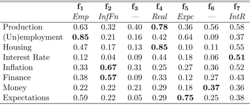
One of the common issues associated with factor-based forecasting approaches is the number of factors to be extracted from the auxiliary data set. To set this in stone, we start by per-forming the information criteria developed by Bai and Ng (2002), and used by Ludvigson and Ng (2009a,c) and Bai and Ng(2011).6 The criteria find eight factors in the Stock and Watson data set. Factors are identified up to a rotation, so a comprehensive interpretation of extracted factors is not straightforward. Stock and Watson(2002a) andLudvigson and Ng (2009c) report marginalR2s of the regressions of each of the series against each of the eight factors they infer from the information criteria. In line with their pre-classification of the dataset, they relate these factors with real economy, output and unemployment series, Treasury Bills, commodity prices and such. Note, however, that the forecasting procedure does not hinge on this classification. For a closer look on the number of factors, we employ the tailored AICL for a preliminary check of the number of factors for the full time span. This preliminary exercise starts with selecting among the 8 largest PCA-extracted factors which are chosen by theBai and Ng(2002) information criteria. In the second step, 9 factors are extracted from the auxiliary data and selection is conducted among these 9, and so on. We stop at selection among the 15 largest
6
Bai and Ng(2002) information criteria donot consider generalised loss functions. We apply these criteria to give a preliminary idea about the number of the factors.
PCA-extracted factors. The factors in each step are used in the predictive regressions to forecast all four variables of interest after being subject to the model selection. The potential forecast relevance of the factors then assessed; Table 1.1 reports the model (i.e. the factors) chosen by minimizing AICL among all factors in that particular step. The loss function is asymmetric quadratic withp= 2 and α∈ {0.1,0.3,0.5,0.7,0.9}.
As shown in the columns of Table 1.1, not all factors in each step are selected as predictors, at least for the full data span. For example, for forecasting P I, in case of α= 0.1, all but fourth factor are selected when selecting among the first 8 factors in total. For the same variable, when
α = 0.5, the forth and sixth factors are not identified as forecast relevant in the first step. For all α, it turns out that the first 8 factors given by the information criteria are not all forecast-relevant.7 Increasing the number of factors to select from one by one, the already selected factors do not generally change. In the last step of our exercise, we contemplate all 15 PCA-extracted factors and note that some of the additional ones appear to be forecast relevant, while some of the commonly used 8 largest factors do not. Changes on the selected factors are observed depending on the chosen α values. This emphasises the differences on the relative importance of the factors which changes with the loss function.
Evidence from this preliminary exercise suggests that the 9th factor is rarely chosen by the tailored AICL while forecasting P I and P I. On the contrary, it is consistently chosen in the cases of U N and SL, for all α values. Additionally, factors beyond 9 appear to be forecast relevant. Thus, we use 15 factors (the largest PCA-extracted ones) as benchmark rather than 8 largest factors found by the information criteria. To keep the complexity tractable, we do not consider classical factors beyond these.
The extracted volatility factor(s) give(s) information which is not (linearly) contained in the original series. According to the mentioned information criteria,8 the PCA of the log-squared residuals from the first-step factor analysis leads to only one additional factor to be taken into account. We consider it as a predictor along with the factors extracted from the data in the first step. While selecting the concrete predictive model for a given span of observations, the volatility factor is subject to model selection with the tailored AIC alongside the other factors. We also consider the squared volatility factor to better account for nonlinearities.
7The objective function of the AIC
Ltargets the dependent variable whereas the PCA analysis aims to
max-imize the variance explained by factors. Due to the difference in the objective functions, the factors selected by the information criteria do not always appear to be forecast relevant.
8Following Bai and Ng (2002), we rely on P C
p2 and P Cp3 as the other criteria tend to – unrealistically –
r
1
Table 1.1. Factors selected for predicting for all predictor series by AICL; full data span
α= 0.1 α= 0.3 α= 0.5 α= 0.7 α= 0.9 8 9 10 11 12 13 14 15 8 9 10 11 12 13 14 15 8 9 10 11 12 13 14 15 8 9 10 11 12 13 14 15 8 9 10 11 12 13 14 15 P er so na l Inco me 1 1 1 1 1 1 1 1 1 1 1 1 1 1 1 1 1 1 1 1 1 1 1 1 1 1 1 1 1 1 1 1 1 1 1 1 1 1 1 1 2 2 3 2 2 2 2 2 2 2 2 2 2 2 2 2 2 2 2 2 2 2 2 2 2 2 2 2 2 2 2 2 2 2 2 2 2 2 2 2 3 3 5 5 3 3 3 3 3 3 3 3 3 3 3 3 3 3 3 3 3 3 3 3 3 3 3 3 3 3 3 3 3 3 3 3 3 3 3 3 5 5 6 6 5 5 5 5 5 5 5 5 5 5 5 5 5 5 5 5 5 5 5 5 5 5 5 5 5 5 5 5 7 7 5 4 4 4 4 4 6 6 7 7 6 6 6 6 6 6 6 6 6 6 6 6 7 7 7 6 6 6 6 6 7 7 7 7 7 7 7 6 8 8 7 5 5 5 5 5 7 7 8 8 7 7 7 7 7 7 7 7 7 7 7 7 8 8 8 7 7 7 7 7 8 8 8 8 8 8 8 7 8 7 7 7 7 7 8 8 10 10 8 8 8 8 8 8 8 8 8 8 8 8 10 8 8 8 8 8 10 10 10 10 10 8 10 8 8 8 8 8 11 9 10 10 10 10 10 10 10 10 10 10 10 10 10 10 11 11 11 11 10 10 10 10 10 10 10 11 11 11 11 11 11 11 11 11 11 11 11 11 12 12 12 11 11 11 11 11 11 11 12 12 12 12 12 12 12 12 12 12 12 13 13 12 12 12 12 12 12 13 13 13 13 13 13 13 13 13 14 13 13 13 13 14 14 14 14 14 14 14 14 14 15 15 15 15 15 I ndust r ia l Pr o duct ion 1 1 1 1 1 1 1 1 1 1 1 1 1 1 1 1 1 1 1 1 1 1 1 1 1 1 1 1 1 1 1 1 1 1 1 1 1 1 1 1 2 2 2 2 2 2 2 2 2 2 2 2 2 2 2 2 2 2 2 2 2 2 2 2 2 2 2 2 2 2 2 2 2 2 2 2 2 2 2 2 3 3 3 3 3 3 3 3 3 3 3 3 3 3 3 3 3 3 3 3 3 3 3 3 3 3 3 3 3 3 3 3 3 3 3 3 3 3 3 3 4 4 4 4 4 4 4 4 4 4 4 4 4 4 4 4 4 4 4 4 4 4 4 4 4 4 4 4 4 4 4 4 4 4 4 4 4 4 4 4 5 5 5 5 5 5 5 5 5 5 5 5 5 5 5 5 5 5 5 5 5 5 5 5 5 5 5 5 5 5 5 5 5 5 5 5 5 5 5 5 6 6 7 6 6 6 6 6 6 6 6 6 6 6 6 6 6 6 6 6 6 6 6 6 6 6 6 6 6 6 6 6 6 6 6 6 6 6 6 6 7 7 8 7 7 7 7 7 7 7 7 7 7 7 7 7 7 7 7 7 7 7 7 7 7 7 7 7 7 7 7 7 7 7 7 7 7 7 7 7 8 8 9 8 8 8 8 8 8 8 8 8 8 8 8 8 8 8 8 8 8 8 8 8 8 8 8 8 8 8 8 8 8 8 8 8 8 8 8 8 10 9 10 10 10 10 10 10 10 10 10 10 10 10 10 10 10 10 10 10 10 10 10 10 10 10 10 10 10 10 11 11 11 11 11 11 11 11 11 11 11 11 11 11 11 11 11 11 11 11 11 11 11 11 11 12 12 12 12 12 12 12 12 12 12 12 12 12 12 12 12 12 12 12 12 13 13 13 13 13 13 13 13 13 13 13 13 15 15 15 14 14 15 U nempl o y men t Ra t e 1 1 1 1 1 1 1 1 1 1 1 1 1 1 1 1 1 1 1 1 1 1 1 1 1 1 1 1 1 1 1 1 1 1 1 1 1 1 1 1 2 2 2 2 2 2 2 2 2 2 2 2 2 2 2 2 2 2 2 2 2 2 2 2 2 2 2 2 2 2 2 2 2 3 2 2 2 2 2 2 3 3 7 4 3 3 3 3 3 3 3 3 3 3 3 3 3 3 3 3 3 3 3 3 3 3 3 3 3 3 3 3 3 6 3 3 3 3 3 3 4 4 8 6 4 4 4 4 6 6 6 6 6 6 6 6 6 6 6 6 6 6 6 6 6 6 6 6 6 6 6 6 6 7 6 6 6 6 6 6 6 6 9 7 6 6 6 6 7 7 7 7 7 7 7 7 7 7 7 7 7 7 7 7 7 7 7 7 7 7 7 7 7 8 7 7 7 7 7 7 7 7 10 8 7 7 7 7 8 8 8 8 8 8 8 8 8 8 8 8 8 8 8 8 8 8 8 8 8 8 8 8 8 9 8 8 8 8 8 8 8 8 9 8 8 8 8 9 9 9 9 9 9 9 9 9 9 9 9 9 9 9 9 9 9 9 9 9 9 9 9 9 9 9 9 10 9 9 9 9 10 10 10 10 10 10 10 10 10 10 10 10 10 10 10 10 10 10 10 10 10 10 10 10 11 10 10 10 10 11 11 11 11 11 11 11 11 11 11 11 11 11 11 11 11 11 11 11 11 11 11 11 11 12 12 12 12 12 12 12 12 12 12 12 12 12 12 12 12 12 12 12 12 13 13 13 13 13 13 13 13 13 13 13 13 13 13 13 14 14 14 14 14 14 14 14 14 14 15 15 15 15 R eta il Sal es 1 1 1 1 1 1 1 1 1 1 1 1 1 1 1 1 1 1 1 1 1 1 1 1 1 1 1 1 1 1 1 1 1 1 1 1 1 1 1 1 2 2 2 2 2 2 2 2 2 2 2 2 2 2 2 2 2 2 2 2 2 2 2 2 2 2 2 2 2 2 2 2 2 2 2 2 2 2 2 2 3 3 3 3 3 3 3 3 3 3 3 3 3 3 3 3 4 4 3 3 3 3 3 3 4 4 4 4 4 3 4 4 4 4 4 4 4 4 4 4 4 4 4 4 4 4 4 4 4 4 4 4 4 4 4 4 5 5 4 4 4 4 4 4 5 5 5 5 5 4 5 5 5 5 5 5 5 5 5 5 5 5 5 5 5 5 5 5 5 5 5 5 5 5 5 5 6 6 5 5 5 5 5 5 6 6 6 6 6 5 6 6 6 6 6 6 6 6 6 6 6 6 6 6 6 6 6 6 6 6 6 6 6 6 6 6 7 7 6 6 6 6 6 6 7 7 7 7 7 6 7 7 7 7 7 7 7 7 7 7 7 7 7 7 7 7 7 7 7 7 7 7 7 7 7 7 8 8 7 7 7 7 7 7 8 8 8 8 8 7 8 8 8 8 8 8 8 8 8 8 8 8 8 8 8 8 8 8 8 8 8 8 8 8 8 8 9 8 8 8 8 8 8 9 9 9 9 8 9 9 9 9 9 9 9 9 9 9 9 9 9 9 9 9 9 9 9 9 9 9 9 9 9 9 9 9 9 10 10 10 9 10 10 10 10 10 10 10 10 10 10 10 10 10 10 10 10 10 10 10 10 10 10 10 10 10 10 12 10 12 12 12 12 12 12 11 11 11 12 11 11 11 11 11 11 11 11 11 11 11 12 13 13 13 13 13 12 12 13 12 12 12 12 12 12 12 12 12 13 14 14 14 14 13 14 13 13 13 13 13 13 13 15 15 14 14 14 14 14 15 15 15
Notes: Asymmetric quadratic loss; see the text for details. The number of factors considered given a particularαand variable are given in bold. The analysis is for the whole time span.
1.4.3 Results
In this section, we discuss the results when model selection is conducted with the tailored information criterion AICL. For each α, we first estimate the respective predictive regression by ordinary least squares (OLS) relying on the regressors in the benchmark models in recursive manner. We construct one-year-ahead forecasts in each given step and evaluate the occurring loss via the forecast errors under the relevant loss function. This approach is henceforth named as OLS-Asymmetric Loss (OLS−AL). The second route to take here is estimating the regression coefficients numerically directly by the aggregated observed loss and using them to construct forecasts. This approach is named as Asymmetric Loss (AL) henceforth. For each variable of interest, first OLS−AL losses are presented and followed by the AL losses. For α = 0.5, the results of consecutive columns are the same, since for p = 2 and α = 0.5 the quadratic loss is recovered.
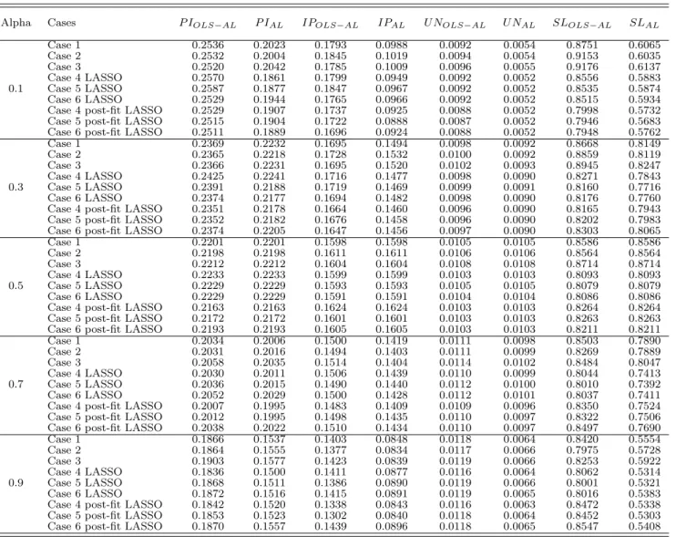
Concentrating on the evaluation of the forecasts obtained using OLS vs. those obtained via estimation under the relevant loss, one expects the average forecast loss of AL to be smaller than the loss which occurs underOLS−AL; see the early work ofWeiss and Andersen(1984). We consider six cases in total. The first case uses only 15 factors for the forecasting exercise. The second case also includes the factor extracted from the log-squared idiosyncratic components b
ut,i. Thus, there are in total 16 factors for this case. The third case adds the squared volatility
factor after which we end up with 17 factors. We do not conduct model selection for Case 1, Case 2 or Case 3. Case 4 is the counterparty of Case 1 with model selection by the tailored AICL. Similarly, Case 5 and 6 are model selection versions of Case 2 and 3, respectively. Note that the model selection is performed in each recursive step. Moreover, one lag of the dependent variable is added to the set of predictors in all cases (and is subject to model selection in Cases 4, 5 and 6). A second lag did not improve forecasting ability in any of the cases or for any of the loss functions so we do not present those results here. Appendix 1.C contains the additional results based on LASSO and post-fit LASSO model selection and estimation.
Table 1.2 summarizes the pseudo out-of-sample average forecast loss for each of the six cases. We fix p = 2 and allow for different degrees of asymmetry by considering five αs for the loss function in Equation (1.2). For each of the six cases we consider, the goal is to forecastP I,IP,
U N and SL under two alternatives of forecast evaluation.
Evaluating the forecasts by the asymmetric loss function of choice leads to lower average losses with the only exception of forecastingIP withα= 0.7 in Case 5.9
In some cases, we see that adding one extra factor, the volatility factor, improves the forecast accuracy. OLS −AL and AL losses reported in case of α = 0.1 numerically demonstrate the
9
Table 1.2. Losses Evaluated for OLS-Asymmetric Loss and Asymmetric Loss
Alpha Cases P IOLS−AL P IAL IPOLS−AL IPAL U NOLS−AL U NAL SLOLS−AL SLAL
0.1 Case 1 0.2536 0.2023 0.1793 0.0988 0.0092 0.0054 0.8751 0.6065 Case 2 0.2532 0.2004 0.1845 0.1019 0.0092 0.0054 0.8978 0.6089 Case 3 0.2520 0.2042 0.1785 0.1009 0.0093 0.0055 0.8896 0.6129 Case 4 0.2493 0.1866 0.1852 0.0913 0.0086 0.0054 0.8236 0.6023 Case 5 0.2502 0.1872 0.1853 0.0911 0.0086 0.0054 0.8236 0.6023 Case 6 0.2501 0.1871 0.1832 0.0935 0.0086 0.0054 0.8236 0.6023 0.3 Case 1 0.2369 0.2232 0.1695 0.1494 0.0098 0.0092 0.8668 0.8149 Case 2 0.2365 0.2218 0.1728 0.1532 0.0099 0.0093 0.8794 0.8158 Case 3 0.2366 0.2231 0.1695 0.1520 0.0100 0.0093 0.8805 0.8220 Case 4 0.2345 0.2179 0.1650 0.1369 0.0094 0.0089 0.8235 0.7895 Case 5 0.2345 0.2179 0.1650 0.1369 0.0094 0.0089 0.8235 0.7895 Case 6 0.2345 0.2179 0.1655 0.1372 0.0094 0.0089 0.8235 0.7895 0.5 Case 1 0.2201 0.2201 0.1598 0.1598 0.0105 0.0105 0.8586 0.8586 Case 2 0.2198 0.2198 0.1611 0.1611 0.0106 0.0106 0.8611 0.8611 Case 3 0.2212 0.2212 0.1604 0.1604 0.0107 0.0107 0.8714 0.8714 Case 4 0.2162 0.2162 0.1419 0.1419 0.0099 0.0099 0.7930 0.7930 Case 5 0.2162 0.2162 0.1419 0.1419 0.0099 0.0099 0.7930 0.7930 Case 6 0.2162 0.2162 0.1419 0.1419 0.0099 0.0099 0.7934 0.7934 0.7 Case 1 0.2034 0.2006 0.1500 0.1419 0.0111 0.0098 0.8503 0.7890 Case 2 0.2031 0.2016 0.1494 0.1403 0.0113 0.0099 0.8427 0.7948 Case 3 0.2058 0.2035 0.1514 0.1404 0.0114 0.0100 0.8623 0.8086 Case 4 0.1980 0.1968 0.1288 0.1286 0.0106 0.0093 0.8033 0.7355 Case 5 0.1980 0.1968 0.1289 0.1292 0.0106 0.0093 0.8034 0.7389 Case 6 0.1980 0.1968 0.1293 0.1286 0.0106 0.0094 0.8033 0.7387 0.9 Case 1 0.1866 0.1537 0.1403 0.0848 0.0118 0.0064 0.8420 0.5554 Case 2 0.1864 0.1555 0.1377 0.0834 0.0121 0.0066 0.8244 0.5674 Case 3 0.1903 0.1577 0.1423 0.0839 0.0121 0.0065 0.8531 0.5840 Case 4 0.1936 0.1484 0.1194 0.0819 0.0114 0.0063 0.8122 0.5309 Case 5 0.1936 0.1484 0.1193 0.0835 0.0116 0.0064 0.8091 0.5357 Case 6 0.1936 0.1484 0.1224 0.0816 0.0114 0.0065 0.8109 0.5356
Notes: The losses are evaluated using asymmetric quadratic loss functions within a recursive pseudo-out-of-sample setup. See the text for details. The dataset for factor extraction includes the dependent variables.
improvement from Case 1 to Case 2. Due to the exceptions, this cannot be generalised over all cases and all variables. Adding the squared volatility factor improves the forecasts of some variables under different loss forecast asymmetries, such as forP IOLS−AL forα = 0.1. However,
for the same asymmetry switching from Case 2 to Case 3 in AL, P I forecast losses point out otherwise, illustrated by increasing forecast losses with the inclusion of this additional factor. We shape our analysis to proceed with forecasting four macroeconomic variables with forecast relevant factors. As shown in Table 1.2, selecting among all the factors included in the system results with smaller forecast losses. Comparisons of Case 1 and 4, Case 2 and 5 and Case 3 and 6 point out that variable selection leads to smaller losses. Given the small number of exceptions10, the analysis addresses strong evidence for variable selection by the tailored information criterion
10
The exceptions are OLS−AL IP Cases 4, 5 and 6 forα= 0.1. P IOLS−AL Cases 4, 5 and 6 forα= 0.9.
AICL being useful.
Our analysis is not designed to select an “optimal”α, since α is imposed by the beneficiary of the forecast i.e. the corresponding loss preferences. Yet, our results can still deliver some insight on the matter. For forecasting unemployment rate, α = 0.1 appears to be the optimal value which leads to the smallest forecast losses for all cases. For the other three variables, α = 0.9
results with the smallest forecast errors for all cases.
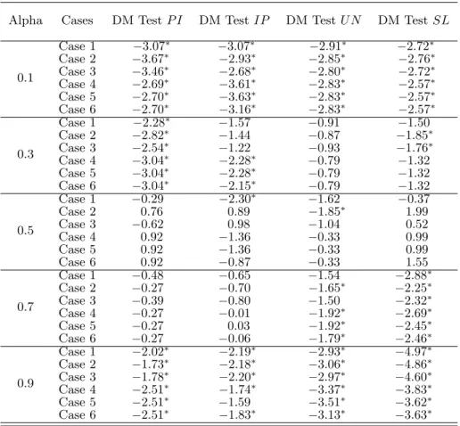
We additionally compared theOLS−ALandALforecasts with the help of the Diebold-Mariano [DM] test for predictive accuracy (Diebold and Mariano,1995). The null hypothesis is that the expected forecast loss is equal for both procedures of interest,y˜(1)t+h andy˜t(2)+h. The losses implied by these forecasts are L(˜vt(1)+h) and L(˜vt(2)+h). Under the null hypothesis, H0 : E
L(˜vt(1)+h) = EL(˜vt(2)+h) or H0 : E(dt) = 0 where dt = L(˜vt(1)+h)− L(˜vt(2)+h) is the loss differential, the DM
test statistic isS =d¯/(LRV[( ¯d)/T¯)0.5∼N(0,1)where T¯ is the number of forecast errors available
for comparison and LRV[ is an estimate of the asymptotic (long-run) variance of
√
¯
Td¯. Since we compute differences betweenALand OLS−AL, we may expect test statistics to be smaller than -1.645 at the 5%significance level whenOLS−AL is inferior.
Table 1.3. Tests of equal predictive accuracy of OLS and AL based forecasts
Alpha Cases DM TestP I DM TestIP DM TestU N DM TestSL
0.1 Case 1 −3.07∗ −3.07∗ −2.91∗ −2.72∗ Case 2 −3.67∗ −2.93∗ −2.85∗ −2.76∗ Case 3 −3.46∗ −2.68∗ −2.80∗ −2.72∗ Case 4 −2.69∗ −3.61∗ −2.83∗ −2.57∗ Case 5 −2.70∗ −3.63∗ −2.83∗ −2.57∗ Case 6 −2.70∗ −3.16∗ −2.83∗ −2.57∗ 0.3 Case 1 −2.28∗ −1.57 −0.91 −1.50 Case 2 −2.82∗ −1.44 −0.87 −1.85∗ Case 3 −2.54∗ −1.22 −0.93 −1.76∗ Case 4 −3.04∗ −2.28∗ −0.79 −1.32 Case 5 −3.04∗ −2.28∗ −0.79 −1.32 Case 6 −3.04∗ −2.15∗ −0.79 −1.32 0.5 Case 1 −0.29 −2.30∗ −1.62 −0.37 Case 2 0.76 0.89 −1.85∗ 1.99 Case 3 −0.62 0.98 −1.04 0.52 Case 4 0.92 −1.36 −0.33 0.99 Case 5 0.92 −1.36 −0.33 0.99 Case 6 0.92 −0.87 −0.33 1.55 0.7 Case 1 −0.48 −0.65 −1.54 −2.88∗ Case 2 −0.27 −0.70 −1.65∗ −2.25∗ Case 3 −0.39 −0.80 −1.50 −2.32∗ Case 4 −0.27 −0.01 −1.92∗ −2.69∗ Case 5 −0.27 0.03 −1.92∗ −2.45∗ Case 6 −0.27 −0.06 −1.79∗ −2.46∗ 0.9 Case 1 −2.02∗ −2.19∗ −2.93∗ −4.97∗ Case 2 −1.73∗ −2.18∗ −3.06∗ −4.86∗ Case 3 −1.78∗ −2.20∗ −2.97∗ −4.60∗ Case 4 −2.51∗ −1.74∗ −3.37∗ −3.83∗ Case 5 −2.51∗ −1.59 −3.51∗ −3.62∗ Case 6 −2.51∗ −1.83∗ −3.13∗ −3.63∗
Notes: The null hypothesis for the test isH0:E[dt] = 0wheredt=L(ˆvt+h)− L(˜vt+h)withˆvt+h the forecast errors from OLS based forecasts andv˜t+hthe asymmetric loss forecast errors. For the one sided test with the alternative hypothesisH0:E[dt]>0, the test statistic should be smaller than -1.645 for 5%significance. Significant outcomes are marked with an asterisk.
Table 1.3 reports the DM statistics of the comparison between the OLS based forecasts and Asymmetric Loss based forecasts. The test statistics confirm our expectations for α = 0.1
without any exceptions. Except forP I, test statistics are insignificant forα= 0.3. The forecasts are not significantly better or worse for α = 0.5 11 but remain insignificant for α = 0.7 except significant results for Sales. Forα being0.9the test gives significant results for all six cases and all variables.
1.5
Concluding remarks
The forecasting literature often focusses on MSE-optimal forecasts. Yet there is evidence em-phasising the relevance of more general loss functions in concrete situations. In this paper, we incorporate some aspects of forecasting under asymmetric loss functions in factor-based predic-tive regressions. First, we show that one may estimate predicpredic-tive regressions under the relevant loss by plugging in factors extracted from a data set by means of a first-step principal components analysis. The estimated optimal forecast from the feasible regression converges in probability to the theoretical optimal forecast. Second, we address the relevance of the estimated factors by assessing whether they are forecast-relevant under a given loss function. To this end, we employtailored information criteria and consider the factors with highest predictive powers for forecasting purposes. Moreover, we argue that principal component analysis does not always extract all relevant information: we analyze the variability of the predictor series and include corresponding additional information in the forecasting model, namely a factor extracted from the log-squared idiosyncratic components estimated in the first-step PCA.
We then illustrate the discussion by forecasting the Personal Income, Industrial Production, Unemployment Rate and Retail Sales series from the Stock and Watson data set. We resort to a recursive pseudo out-of-sample forecast evaluation scheme where the factors are extracted from a subset of the Stock and Watson data and used for forecasting one-year-ahead values ofP I,IP,
U N andSLunder several asymmetric power loss functions. We compare six forecasting models (Case 1: fifteen factors; Case 2: fifteen factors and the volatility factor; Case 3: fifteen factors, the volatility factor and squared volatility factor, Case 4: selection of forecast-relevant factors among fifteen, Case 5: selection of forecast-relevant factors among sixteen, Case 6: selection of forecast-relevant factors among seventeen) for different parameter values when the p = 2
is fixed. Expectedly, fitting the forecasting model under the relevant loss function leads to smaller averaged losses compared to the case when we use MSE in the majority of cases. Adding
11
The loss differential should be zero when α= 0.5 and p= 2 as OLS−ALand ALare identical for this particular case. TheOLS−ALand theALestimators forα= 0.5are however computed in a different manner (via the QR decomposition for OLS and by numerical optimization for AL), hence some negligible numerical differences arise resulting in non-zero but insignificant DM statistics.
volatility information sometimes improves the forecasts. Model selection taking the relevant loss into account leads to overall best results.
Both our theoretical and empirical results underscore the importance of using forecast-relevant information by estimating factors from an auxiliary data set to exploit the additional information (i.e. the volatility factor in our case). Also relevant, if not even more so, is the issue of choosing the most relevant information for the particular loss function used to define optimality of the forecast.
Appendix 1
1.A
An information criterion
Following Akaike (1973), the definition of the information criterion in form of a penalized log-likelihood leads to
AIC(k) =−2 lnLˆ(k)+ 2k
withLˆ(k) denoting the maximum of the likelihood function for model complexity k.
Suppose now that the error term in the model of interest follows an asymmetric (exponential) power distribution as characterized by Ayebo and Kozubowski (2003) and Komunjer (2007)12 with density function
f(v) = δ 1 λ σΓ1 +λ1 e−δ 1 αλ∗I(v≤0)+ 1 (1−α∗)λI(v>0) |v σ| λ where δ = 2αλ∗(1−α∗)λ αλ
∗+(1−α∗)λ. Quasi-ML estimation of a regression model assuming vt ∼ f is then
easily shown to be equivalent to estimation under the loss function L with parameters p = λ
and α= (1−α∗)p
(1−α∗)p+αp∗.
After concentrating outσ, some algebra leads to
AICL(k) = 2 pln X L(ˆvt+h) +2k T
withvˆt the residuals from estimation of the predictive regression under the relevant lossL.
This reduces to the AIC whenL is the squared-error loss function. Note that AICL differs from the IC proposed by (Weiss, 1996, Section 5) in two important respects. First, Weiss focusses on comparing forecasts from models based on different loss functions, while we are interested in selecting the best forecasting model for a given loss function; second, the expression he arrives at is not scale invariant, whereas, for the loss function in (1.2), AICL is.
1.B
Proof of Proposition 1
Note first thatL is continuous and piecewise linear forp= 1, while, for p >1 it is smooth with continuous and piecewise linearp−1st order derivative.
12
They introduce asymmetry in the exponential power (also generalized power, or generalized error) distribution by using the method discussed inFernandez et al.(1995). An alternative way of “skewing” the exponential power distribution is based on the approach ofAzzalini(1985).
The target function is given by Qa∗j, b∗k, c∗, aj, b