Journal of Marketing Research
Vol. XLVIII (June 2011), 425 –443 *Zsolt Katona is Assistant Professor of Marketing, Haas School of
Busi-ness, University of California, Berkeley (e-mail: [email protected]. edu). Peter Pal Zubcsek is Assistant Professor of Marketing, University of Florida (e-mail: [email protected]). Miklos Sarvary is Professor of Marketing, INSEAD (email: [email protected]). Peter Pal Zub -csek’s work was supported by the Sasakawa Young Leaders Fellowship Fund. The authors acknowledge Hubert Gatignon; Andrew Stephen; Christophe Van den Bulte; Miguel Villas-Boas; and seminar participants at Marketing Science, Rotterdam School of Management, and INSEAD for their invaluable comments and suggestions. Wayne DeSarbo served as associate editor for this article.
ZSOLT KATONA, PETER PAL ZUBCSEK, and MIKLOS SARVARY*
This article discusses the diffusion process in an online social network given the individual connections between members. The authors model the adoption decision of individuals as a binary choice affected by three factors: (1) the local network structure formed by already adopted neighbors, (2) the average characteristics of adopted neighbors (influencers), and (3) the characteristics of the potential adopters. Focusing on the first factor, the authors find two marked effects. First, an individual who is connected to many adopters has a greater adoption probability (degree effect). Second, the density of connections in a group of already adopted consumers has a strong positive effect on the adoption of individuals connected to this group (clustering effect). The article also records significant effects for influencer and adopter characteristics. For adopters, specifically, the authors find that position in the entire network and some demographic variables are good predictors of adoption. Similarly, in the case of already adopted individuals, average demographics and global network position can predict their influential power on their neighbors. An interesting counterintuitive finding is that the average influential power of individuals decreaseswith the total number of their contacts. These results have practical implications for viral marketing, a context in which a variety of technology platforms are increasingly considering leveraging their consumers’ revealed connection patterns. The model performs particularly well in predicting the next set of adopters.
Keywords: diffusion, social networks, network marketing
Network Effects and Personal Influences:
The Diffusion of an Online Social Network
© 2011, American Marketing Association
ISSN: 0022-2437 (print), 1547-7193 (electronic) 425 Although marketers have long recognized the importance of word of mouth (WOM) in influencing consumer deci-sions, it has been difficult to measure the impact of WOM and to use it efficiently for commercial purposes until recently. Modern technology, however, has gradually trans-formed social interactions among people. On average, people spend more time communicating with the help of technology
platforms (e.g., phone, VoIP [voice over Internet protocol], e-mail, chat), and their frequent contacts are readily avail-able to the owners of these communication platforms. With the emergence of Web 2.0 technologies, media such as blogs, instant messaging (e.g., msn.com), and social net-working websites (e.g., Facebook.com) are becoming ubiq-uitous, and they all provide a “map” of communication paths among their users. Social networking sites such as MySpace and Facebook are particularly interesting exam-ples. They represent rich and popular communication inter-faces for hundreds of millions of users. On these sites, users exhibit their demographics as well as their preferences by carefully editing (decorating) their profiles. More important, they explicitly link to their friends and, in doing so, reveal their likely communication patterns. In the past five years, social networks have populated the world, often attracting a critical proportion of a country’s population. Cyworld, for example, claims to count more than 40% of Koreans among Reprinted with permission from the Journal of Marketing Research, published by the American Marketing Association.
its membership base, whereas Facebook has more than 400 million members worldwide, recently surpassing Google in becoming the most visited website in the United States.
The increased importance of technology platforms for social interactions has raised the interest of product marketers who want to explore them as new advertising/promotion media. Indeed, social networks’ revenue models are based primarily on advertising, though so far, the use of (mostly) banner-type advertising has produced disappointing results (e.g., BusinessWeek2008; The Economist2007). Marketers increasingly believe that the efficient way of using social net-works for marketing relies on harnessing WOM by analyzing the network of members’ connections. For example, Google recently filed a patent for an algorithm that identifies so-called influencers on social networks. Several other firms (e.g., Idiro, Xtract) provide network analysis for the telecom-munications sector and for various Web 2.0 platforms to assist in viral marketing campaigns. Indeed, social networks represent but one area in which network analysis might be used for WOM marketing. Other technologies (e.g., blogs, telecommunications, virtual worlds) that record consumers’ communication patterns are also adapted to such techniques. In all these cases, the essential idea is that understanding the network structure of individual consumers can help imple-ment effective viral marketing strategies.
The assumption that underlies all these “network-marketing” techniques is that network information can help identify influencers and predict consumers’ adoption probabilities. The goal of this article is to verify this assumption and iden-tify how the network structure drives adoption. To be spe-cific, we develop and empirically test an individual-level diffusion model that explicitly takes into account the microstructure of interpersonal connections among poten-tial adopters. Our empirical application studies the growth of a country-specific social network site for which member-ship can be acquired only by receiving an invitation from an existing member. In this context, we study the adoption process of network memberships at an early stage of the site’s development. We assume that the social network site gradually replicates people’s real-life social connection pat-terns. Thus, by recording the site’s membership network at a much later point in time, we can assume that it reflects people’s real-life social networks accurately. Then, we can retroactively observe a diffusion process of membership on this “ultimate” or “final” network.1
Our primary research objective is to uncover the effects of differences in individuals’ connection patterns on the dif-fusion process. Motivated by both conceptual and practical considerations, we distinguish three factors that may affect a potential adopter’s adoption decision. The first factor, which we call “network effects,” relates to the influence of the structure of connection patterns of the potential adopter’s already adopted neighbors. The second factor, which we call “influencer effects,” refers to the (average) individual characteristics of already adopted network
mem-bers on their not-yet-adopted neighbors. In contrast to the previous factor, which concentrates on the impact of the structure, for influencer effects we essentially measure the (average) influential power of every adopter. The average characteristics that describe influencers may be demograph-ics, such as age, but they also may include measures that describe the global network position of the influencers— that is, their position in the final social network observed. The third factor, called “adopter effects,” captures the effects of the adopter’s individual characteristics. For influ-encers, these characteristics include both demographics and characteristics that describe the adopter’s global network position. Depending on data availability and legislative con-straints, marketers can use each of these categories of vari-ables to identify potential marketing targets to influence the adoption process. They can target members of the network who have already adopted the promoted product or poten-tial adopters who have yet to adopt. In both cases, potenpoten-tial marketing targets can be selected on the basis of their indi-vidual characteristics or, alternatively, of the local network structure that surrounds them. Our model helps identify potential adopters by predicting the next set of adopters sub-stantially better than models based solely on demographic variables.
In our choice of network variables, we rely on diffusion theory and previous research in sociology. In particular, indi-viduals who are related to many already adopted members may have greater adoption probability because their related partners can provide more information about the service or innovation in question and ultimately exercise greater joint influential power. We call this the “degree effect,” after the number of connections (degree) an individual has. In addi-tion to the number of connecaddi-tions, the density of connecaddi-tions in a group of already adopted users may also affect the adop-tion of individuals being linked to the members of this group. A more tightly connected group should have a stronger influ-ence on its members; we call this the “clustering effect.” We find strong empirical evidence to support the presence of both the degree and clustering effects, as well as a positive interaction between them.
Beyond network effects, we also find strong influencer and adopter effects on the adoption probability of potential network members. For example, some demographic charac-teristics (e.g., age, gender) can predict adopters’ influential power on their neighbors. In a similar way, demographic variables can also predict potential adopters’ propensity to adopt. More interesting is that variables that describe indi-viduals’ position in the social network (e.g., the number of their contacts, how connected these neighbors are, the extent to which they are interconnecting parts of the net-work) are also good predictors of both influential power and adoption propensity. From both theoretical and practical perspectives, a particularly interesting empirical result is that the average influential power of individuals is lower the larger their social network is. This result suggests that hav-ing a high number of friends dilutes the influential power that an individual has on each of his or her friends. We also find some evidence to indicate that the same influential power is greater the more the actors occupy a “brokering” position among their contacts.
We organize the rest of the article as follows. Next, we place our work in the context of the extant literature and 1It is important to realize that we do not study a network growth or
net-work formation process but rather a diffusion process on an already exist-ing network of potential adopters; the results depend on the validity of the assumption that we have indeed captured the relevant social network by observing the membership network at a late stage. In our empirical appli-cation, we test this assumption in various ways (see the “Network Dynam-ics” subsection).
Network Effects and Personal Influences 427 highlight our points of departure. Then, we set up the
sto-chastic network-based diffusion model and introduce the network measures used. We then present our empirical analysis, including extensive validity tests. Finally, we dis-cuss the results, provide our conclusions, and highlight a few limitations.
RELATED LITERATURE
Our work draws on two broad research streams: (1) the marketing literature on new-product diffusion and (2) the sociology literature on social network analysis. The large body of quantitative research on new-product diffusion is based on models that, for the most part, ignore connection patterns among individuals. Like most of its generalizations, the Bass (1969) model implicitly assumes that every con-sumer is connected to every other concon-sumer and estimates a uniform interpersonal influence (interpreted as WOM) on this (assumed-to-be) complete network. This assumption typically also applies to diffusion models that take into account consumer heterogeneity.2Although these models
allow for heterogeneous WOM effects, they still ignore the network structure of the adopter population. Given the cen-tral role of WOM communication for the diffusion process, there has been a call in the literature to incorporate the fine-grained structure of interpersonal connections into diffusion models (see Mahajan 1993; Mahajan, Muller, and Bass 1990). Although various models have been developed to address this call (e.g., Goldenberg, Libai, and Muller 2001, 2002; Shaikh, Rangaswamy, and Balakrishnan 2005; for a review, see Valente 2005), these models could only be tested on aggregate data.3
In recent years, various technological innovations have made it possible to access network data on the interpersonal relationships between consumers. Empirical studies have developed and used models to assess the impact of network characteristics on the diffusion process. For example, Godes and Mayzlin (2004) study how WOM can be a driver of per-sonal preferences in an environment in which consumer communication via newsgroups is observed. Van den Bulte and Lilien (2001) analyze the Medical Innovation data set, which tracks the medical community’s understanding of a new drug. To obtain the structure of WOM, they combined data from two overlaid relationship networks (“discussion” and “advice”) to get a social-influence weight matrix over the doctors whose behavior was recorded. They then esti-mated an individual-level diffusion model to demonstrate that earlier findings on social contagion over the same net-work were confounded with the marketing efforts (pricing and promotion) of the manufacturer. Nair, Manchanda, and Bhatia (2010) study physician prescription behavior and find that opinion leaders in the physician’s reference group may
have a significant influence on the physician’s behavior. In another domain, Hill, Provost, and Volinsky (2006) use telecommunication data to provide evidence that customers who communicated with a customer of a particular service have an increased likelihood of adopting that service. Iyen-gar, Van den Bulte, and Valente (2008) investigate the rela-tionship between self-reported leadership and sociometric leadership, that is, when a person is nominated by others as someone to whom they turn for advice. They find that these two types of opinion leaderships are only weakly correlated and that there are significant differences in the adoption behaviors of different types of opinion leaders. Studying a different type of network, Stephen and Toubia (2010) exam-ine the role of the link structure in seller networks in which links facilitate customers’ navigation between stores. They find that the network had a positive overall effect on store performance and that the position of stores in the network had a significant effect on their profitability.
Our work directly follows this stream of research. Our primary goal is to understand how network characteristics (particular patterns of connections between already adopted network members) may influence the adoption probabilities of their not-yet-adopted peers. To establish this relationship, we estimate a discrete-time proportional hazards model. This approach is the same one that Bell and Song (2007) follow to estimate network effects on purchase behavior across regions in the United States. However, because our data set enables us to observe the individual network con-nections of participants, we are able to use the same approach to study the impact of personal network structure on adoption.
Sociology researchers have extensively studied how net-work structure affects social influence, though only in small social networks.4Krackhardt’s (1998) influential study
sug-gests that when assessing the influence that individuals’ con-tacts have over them, researchers should not only count the number of related actors but also examine how those relation-ships are embedded in the entire network of relationrelation-ships. Coleman (1988) and Burt (2005) establish two important social phenomena, which may be tied to structural properties of the network. When two related individuals are connected to the same third parties, the network becomes more effective at transmitting information, and the affected relationships ultimately become stronger. Burt (2005) labels this “network closure.” He argues that the shared third parties create redun-dant paths for information flow, leading to increased trust between the two related actors. As a consequence, friends of individuals in social networks are typically densely connected to one another compared with the average connectivity in the network (Watts and Strogatz 1998). This result is consistent with those of Granovetter (1973) and Rogers (2003), who state that social networks in general consist of clusters of densely connected individuals with strong ties among them and sparse weak ties connecting such clusters to each other. Burt (2005) highlights another phenomenon related to the structural properties of social networks—namely, that individuals interconnecting these clusters may have greater influence on their peers because they have control over infor-mation that originates from other groups. This phenomenon 2For early papers, see, for example, Oren and Schwartz (1988); Urban
and Hauser (1993); for more recent applications, see, for example, Golden-berg, Libai, and Muller (2002); Van den Bulte and Joshi (2007).
3Goldenberg, Libai, and Muller (2001, 2002) generate adoption data by applying stochastic cellular automata models to simulate the diffusion process on a two-dimensional grid. Goldenberg, Libai, and Muller (2002) compare the results of their simulations with consumer electronics sales data to explain double-peaked diffusion curves, observed in many product categories. Shaikh, Rangaswamy, and Balakrishnan (2005) develop a diffu-sion model that takes into account local network characteristics. They demonstrate how it may be used to infer structural properties of the con-sumer network from aggregate sales data.
4See also relevant early studies in marketing by Reingen and Kernan (1986) and Reingen et al. (1984).
is termed “brokerage,” and the argument is often cited as structural hole theory (Burt 2005). These arguments provide critical input for our network measures.
Our model is based partly on the approaches that Holtz (2004) and Shaikh, Rangaswamy, and Balakrishnan (2005) propose. However, these studies do not estimate the adop-tion process at the individual level. The former author attempts to disaggregate the Bass (1969) model to the net-work level and uses simulations to confirm the results, whereas the latter authors compare the fit of a small-world-based diffusion model with the traditional models using aggregate-level data. In contrast, in the current study, we develop and estimate an individual-level diffusion model in which each individual is described by both his or her local network characteristics and demographic information. At any point during the adoption process and for each potential adopter, we compute the network spanned by his or her already adopted peers. We then estimate how the structure of the network of his or her adopted peers affects the adop-tion probability of the potential adopters. In addiadop-tion, we also show empirically how network characteristics of already adopted individuals may predict their influential power on others. The estimates also provide insights into some of the common sociological theories in network analysis. In the next section, we present our model.
MODEL The Adoption Process
To examine the process of diffusion over a social net-work, we use a hazard-rate model. We assume that all mem-bers of the network are potential adopters of a certain prod-uct or service. The relationships among network members serve as paths for WOM communication, through which network members may influence each others’ adoption. We denote such a social network by G(V, E), where V is the set of potential adopters and E is the set of symmetric binary relationships among members of V.
By neighbors of a potential adopter v, denoted as N(v), we refer to those network members (actors) who are con-nected to v. That is, N(v) = {w | w V and {v, w} E}. The degree of a node, d(v), then the number of its neighbors: d(v) = |N(v)|. For notational convenience, we further define an indicator function of the relationships in the network. For every v1, v2 V, we let
We assume that at the start of the diffusion process, a small set of actors, A0 V, have already adopted the
inno-vation in question. We then model time in a discrete way. In every time step, some actors adopt the innovation, resulting in the series A0 A1 ... AT, where Atdenotes the set of
actors in the network who have adopted the innovation dur-ing the first t steps. For the individuals in the network, let Tv
denote the adoption time of actor v, yielding
It is important to make the distinction between the overall social network and the subnetworks induced by At. The
net-work G(V, E) defined on the entire set of individuals V (the
e(v , v ) if v , v E otherwise. 1 2 = 1 2 1 ( ) 0 ∈ A = vt { ∈V T| v≤t}.
potential adopters) remains unchanged throughout the process. However, as the number of adopters increases over time, Atcovers an increasingly larger subset of V. The
net-work induced by Atconsists of the nodes of Atand links of
the original network G(V, E) leading between two already adopted members (of At). If we were to plot the network
induced by Atfor every t < T, with the overall network in the
background, we could see how the innovation diffused across the network over time.
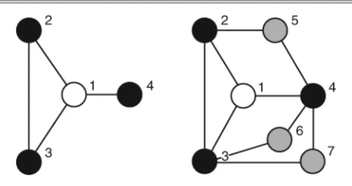
In our model, the adoption likelihood of potential adopters depends on their individual propensity to adopt and on the influence of their neighbors who have already adopted. As explained previously, we distinguish conceptually among three types of influences. First, (local) network effects refer to the impact of the structure of connection patterns among the potential adopter’s already adopted neighbors. Thus, in this case we consider only the networks that are induced by Atfor a given time t. Figure 1 illustrates this phenomenon:
The network among the black nodes 1, 2, and 3 may influ-ence the adoption likelihood of later adopter 8. It is impor-tant to emphasize that these network effects do not distin-guish individuals in the personal networks of potential adopters; only the local network structure drives such effects. Over time, this local network changes as more and more neighbors of the potential adopter adopt themselves. As such, network variables are time-varying covariates.
Second, influencer effects refer to the impact of average individual characteristics of already adopted network mem-bers on their not-yet-adopted friends. These average charac-teristics may be demographics (e.g., age), but they also may include measures that describe the global network position of the influencers—that is, their position in the final friend-ship network, G. Although these measures do not change over time for a single influencer, because we measure the average effect of influencers, these variables also become time-varying covariates as additional influencers adopt the innovation. Influencer effects may affect multiple potential adopters. Figure 2 illustrates this point: The already adopted actor 8 may affect the adoption likelihood of later adopters 9, 10, 12, and 13, indicated by black nodes. We assume that such personal influences are the same on all of the influ-encer’s later-adopting neighbors.
Figure 1
“NETWORK EFFECTS”: ThE SET OF ADOPTED NEIghBORS S = {1, 2, 3} INFLUENCES ThE ADOPTION LIKELIhOOD OF
Network Effects and Personal Influences 429
Finally, we consider adopter effects, which refer to the impact of the adopters’ individual characteristics on their adoption propensity. These are constant variables over time. Again, some of these measures are demographic variables, but we also include the overall network characteristics of a certain adopter, for example, the total number of connec-tions an individual has in the final network, G. (By consid-ering the number of real-life friends an individual has, we control for differences in individuals’ propensity to make friends.) To capture the effects just described, let f denote the influence function f:2vV [0, 1], which we interpret
as follows. If an actor v V has not yet adopted by time t, the probability that it adopts at time (t + 1) is f[N(v) At, v],
that is, a function of the set consisting of the neighbors of the actor who have already adopted and the actor itself. For-mally,
(1)
Thus, the function f(S, v) captures both the propensity of actor v to adopt the innovation in question and the strength of influence the set of adopted neighbors S V has on actor v. (Note that our model formulation also allows for individual characteristics of members of S to influence the adoption likelihood of v.) To estimate the effect of certain structural properties of the network on adoption probabilities, we interpret the daily adoption decisions as binary choices of actors between adoption and nonadoption. There are a num-ber of different link functions that can be used to model such binary decisions as dependent variables, including the
most frequently used logit and probit. We use the comple-mentary log–log link function formulating the equation (2)
where X(S) is a set of variables that describe the local net-work structure, W(S) is a set of variables that describe the average characteristics of the members of S (the influencers), and Z(v) is a set of node-specific (i.e., adopter-specific) covariates. The choice of the complementary log–log trans-formation has two important advantages over the logit and
Pr(T = t + 1|Tv v >t) = f N(v[ )∩A , vt ]. f(S, v xp{ exp[ X(S) + W(S) + Z( ) ≡ 1− − + × × × e α β ϕ γ vv)]},
probit functions. First, the so-derived discrete-time parameter estimates are also the estimates of an underlying continuous-time proportional hazards model (Prentice and Gloeckler 1978). In addition, the complementary log–log link also enables us to directly relate our model to hazard-rate models with utility-maximizing consumers (Bell and Song 2007).
We also note that the complementary log–log and logit formulations yield similar results for small probabilities. However, in addition to enabling a direct interpretation of the results as hazard ratios, the complementary log-log method also provides a slightly better fit in such cases.
Measures
Network effect measures. We begin by discussing the effects that the local structure of already adopted friends has on the adoption likelihood of an individual. We keep the notation S = N(v) Atfor convenience. The first network
effect measure is degree. The most natural question to ask regarding the influence of an actor’s adopted neighbors is how their number affects the likelihood of the actor’s adop-tion. Granovetter (1973) and Valente (2005) suggest that one friend may have a greater impact on an actor’s behavior when the actor has, in total, fewer friends. Thus, we choose our first local network variable to be the proportion of already adopted friends5:
It is intuitive that if a person has more friends already using a certain service or product, he or she will adopt with a greater probability. Thus, we expect degree to have a posi-tive effect on adoption probability.
Our second local network variable is the clustering coef-ficient, which measures the extent to which a set of mem-bers are interconnected. It is clear that this measure might be relevant in a context in which these members exert an influence on another member. The definition of the cluster-ing coefficient is as follows:
where the numerator counts the number of links among the already adopted neighbors of v and the denominator is the maximum number of relationships possible among them. Network closure theory (Burt 2005; Coleman 1988) pro-poses that if two actors related to the same individual are also related to each other, they have greater power over that individual than if they were unrelated. In our context, we could expect that if a potential adopter hears about the social network service from two friends, the attractiveness of the service is greater when these two friends also know each other. Thus, the density of relationships among adopted friends of potential adopters may affect their adop-tion likelihood. On the basis of this stream of research in sociology, we expect that clusteredness has a positive effect on adoption probability. X (S) = |S| |N(v)| 1 . X (S) = (S) = e(s,t) 2 s, t S s, t S ρ ∈ ∈
∑
∑
1 , Figure 2“INFLUENCER EFFECTS”: ChARACTERISTICS OF ACTOR v = 8 AFFECT ThE ADOPTION LIKELIhOOD
OF ALL LATER ADOPTERS w = 9, w = 10, w = 12, w = 131 2 3 4
5Subsequently, we explore an alternative formulation in which we use the number of adopted friends an individual has.
As we already discussed, on average, a higher clustering coefficient indicates stronger relationships. However, keep-ing the density of one’s personal network constant, the num-ber of relationships in the network increases quadratically with the number of related actors. In other words, a larger personal network with the same clustering coefficient requires more ties per neighbor between its members. Therefore, we expect that larger personal networks with the same clustering coefficient indicate a stronger network clo-sure. In other words, we expect a positive interaction effect between the degree and clustering variables. To this end, our third variable becomes the degree–clustering interaction:
Influencer measures. For influencer measures, we focus on the variables that describe the characteristics of the indi-viduals who may influence a potential adopter. The first variable is “influencer total degree.” Opinion leaders have always been a focus for marketers. They are considered important targets for marketing communication. Nair, Man-chanda, and Bhatia (2010) empirically show that in referral networks of physicians, opinion leaders significantly alter the behavior of other individuals in the networks. Studying the aggregate impact of influencers on diffusion, Watts and Dodds (2007) ran a series of computer simulations. They show that the structure of social influence may decrease the relative importance of highly connected individuals over a critical mass of easily influenced individuals. Goldenberg et al. (2009) examine this issue in an empirical study and find that members of a social network with large network degrees (hubs) actually had a larger-than-average overall impact on adoption. In our model, we revisit this question, but we focus strictly on the microlevel effects of high net-work degree. We analyze how the average influence of adopted network members on their later-adopting friends depends on the total number of friends these adopted actors have. That is, our first influencer variable is the average number of connections that potential adopters’ friends have:
Lin (1999) argues that in social networks, the larger the per-sonal network of actors becomes, the easier it is for these actors get access to more diverse social resources. Goldenberg et al. (2006) also find support for this argument: Surveying consumers’ opinion-seeking habits, they identify conditions in which social connectivity is more important for opinion lead-ership than product expertise. In the context of our analysis, however, social status alone is insignificant to influence the behavior of not-yet-adopted individuals: New adopters had to be actively informed about this novel type of service. Personal communication (at least one of the adopted friends sending an invitation, plus perhaps other, potentially offline conversa-tions) had to precede every adoption, and many of the instru-mental actions Lin (1999) mentions were not supported by the medium. For this reason, we argue that the average intensity of friendships of an actor likely diminishes with the number of friends the actor has. This is also consistent with the findings of Stephen, Dover, and Goldenberg’s (2010) recent marketing study and with early sociological work by French and Raven
X (S) = X (S)3 1 ×X (S)2 . W (S) = d(w) S 1 w∈S
∑
| | .(1960), who suggest that people only have a limited amount of influential power. In other words, although it is likely that highly connected individuals have a high degree of influence on their closest ties, it is also likely that they could not spend much time communicating with all of their friends. In sum-mary, we expect that the average influential power of actors (on average over all actors) decreases with the total number of friends the actors has.
The second variable is “betweenness.” Freeman (1977, 1979) defines the “betweenness centrality” of v so that for every pair (s, t) of the other nodes in the network, if v lies on the shortest path between s and t, then that pair of nodes contributes to the betweenness centrality of v. The intuition behind such a definition is that if a message traveling from s to t must pass through v, then the structure of connections indeed increases the influence of v over t (and, in an undi-rected network, over s, because the roles of source and des-tination are interchangeable).
Although such influence may be present in general (e.g., organizational) social networks, we argue that in our net-work of real-life friendships, the influence is irrelevant if s and t are not actually neighbors (friends) of v; that is, we argue that influence depletes rapidly with additional inter-mediaries. Therefore, we propose a definition for local betweenness to focus on structural holes at v by examining only pairs of neighbors of v:
(3)
For every unrelated pair of actors (s, t) among the neighbors of v, the contribution of the pair (s, t) to the betweenness of v is inversely proportional to the number of two-step paths between s and t. For simplicity, hereinafter, we refer to the local betweenness measure as “betweenness.”
Figure 3 illustrates the concept. In the network on the left, actor 1 interconnects the pairs of not-related actors (2, 4) and (3, 4) but not (2, 3), because actors 2 and 3 are related in that network. Because actor 1 is the intermediary of the only two-step path between actors (2, 4) and (3, 4), B(v) in Equa-tion 3 becomes actor 2. In the same figure, on the right-hand side, actor 1 interconnects the same two pairs of not-related actors. However, actors (2, 4) are also connected through actor 5, whereas actors (3, 4) are also connected through
B(v) = e(s, v) e(v, t) [1 e(s, t) e( s t V w V ≠ ∈ ∈
∑
∑
× × − ] ss, w) × e(w, t) . Figure 3SAMPLE NETWORKS TO ILLUSTRATE LOCAL BETWEENNESS
Notes: In the network on the left, the local betweenness of actor 1 is 2, whereas in the network on the right, actor 1’s local betweenness is 5/6.
Network Effects and Personal Influences 431 both actors 6 and 7. In this way, B(v) becomes 1/2 + 1/3 =
5/6.
To account for the effect of local betweenness on the adoption likelihood of v, we take the average betweenness of v’s neighbors at the time of the adoption decision. Thus, our second influencer variable becomes
(4)
How does this variable affect adoption probabilities? Besides network closure, Burt (2005) details another struc-tural pattern of network connections that may alter the influ-ential power of network members involved. When an actor is interconnecting two otherwise not well-communicating parts of a network, we talk about a structural hole in the network. The interconnecting actor may be able to broker information between the two sides. It is clear that such brokers may have greater influence over related actors on both sides of the net-work. Thus, the literature on structural holes would suggest that structural holes increase the influential power of bro-kers. However, when the personal network of an actor has two parts that otherwise do not communicate, the influence of the actor in the middle of the structural hole is governed by two opposing effects. It may increase with the sizes of the corresponding parts because of the greater social status that brokerage gives, but as we pointed out previously, as the per-sonal network grows larger, on average, these relationships become weaker, and the influence of the brokering actor on his or her potential adopter friends may decrease.
Control variables. In addition to the variables outlined previously, we use a number of control variables in our esti-mations. Because of the lack of theory, we do not have explicit predictions on the effect of these measures. How-ever, from a practical perspective, including them in the estimation may be interesting, because they can help predict adoption probabilities and identify influential consumers.
One of our control variables is the influencer’s clustering coefficient in the final friendship network. As we discussed previously, this variable is a proxy for how dense the influ-encer’s network is. Furthermore, we examine the effect of two demographic variables. In particular, we examine how an influencer’s age and gender affect his or her influential power. As in the case of the network variables, we take an average over the neighborhood of the individual. For exam-ple, in the case of age, the variable is as follows:
For gender, we simply include the proportion of females within S.
Adopter measures. This group of variables measures how the characteristics of potential adopters affect their likeli-hood of adoption in each time period. Again, these variables are of two types. The first set describes the adopter’s final network characteristics (total degree, betweenness, and clusteredness), as in the case of influencers. For the lack of theory, we do not have explicit predictions concerning these variables. Rather, they should be considered control vari-ables. The second set of (control) variables is demographics.
W (S) B(w) S 2 = w S | | . ∈
∑
W (S) AGE S 3 w S w = | | . ∈∑
Beyond age and gender, we can also include an additional variable: population density of the city of residence.
EMPIRICAL ANALYSIS Data Description
Our data originate from a major European social net-working site. The goal of this web-based netnet-working serv-ice is to build an online community of people who then may use the tools provided by the website to interact (e.g., to send messages to their friends, to share their pictures, to maintain a profile page with personal information). People can represent their “friendship network” graphically and can search the membership base by various criteria. An impor-tant feature of the site is that proposed friendships need to be confirmed by the other party and can be severed as well. As a result, the network contains information on mutual relationships only.
Today, the portal we study has more than 4 million regis-tered users and more than 100 million friendship links between them. In this article, we analyze adoption data from the first 3.5 years (1247 days) of the service. We consider this early time frame for two reasons: First, during this period, the service was not advertised and its media appear-ance was minimal, which means that membership growth was entirely due to WOM effects; second, during the period studied, the service was the only of its kind in the country. At the end of the examined time period, the website began experiencing technical difficulties providing the service, and its administrators limited the number of new members who could join. Soon after the alleviation of the technical problems, social networking received national media expo-sure, resulting in both the launch of competing portals and a sudden growth of membership.
To register to the site, potential users had to receive an invitation from a member. During the time period we study, a member had unlimited invitations to send; thus, the avail-ability of invitations did not limit the growth of the network. During the period analyzed, 138,964 users registered on the website. To minimize the potential bias caused by including only users who adopted during the studied time frame, we also include some of the next adopters in the data set. Because of computational limitations, we set the size of the analyzed sample at 250,000 users (of whom the latter 111,036 members signed up during the first month after the last day we examine).
When analyzing the diffusion process, we investigate the adoption of the portal (the social network site) over time by members of the real-life friendship network of potential adopters. We consider all the relationships confirmed in the system 36 weeks after the end of the studied period as this real-life friendship network. By doing so, we implicitly assume two things: (1) The network recorded on the site 36 weeks after our study period contains all the “real-life” rela-tionships between potential adopters, and (2) the relation-ships indicated in the network were not “formed on the net-work” (i.e., not even partly resulting from individuals’ adoption behavior). The validity of these assumptions may be critical to our findings. In the subsection “Robustness and Validity Tests,” we conduct several tests to conclude that neither assumption weakens our empirical results.
The friendship data (sampled as described previously) contain 13,152,323 links among the 250,000 registered
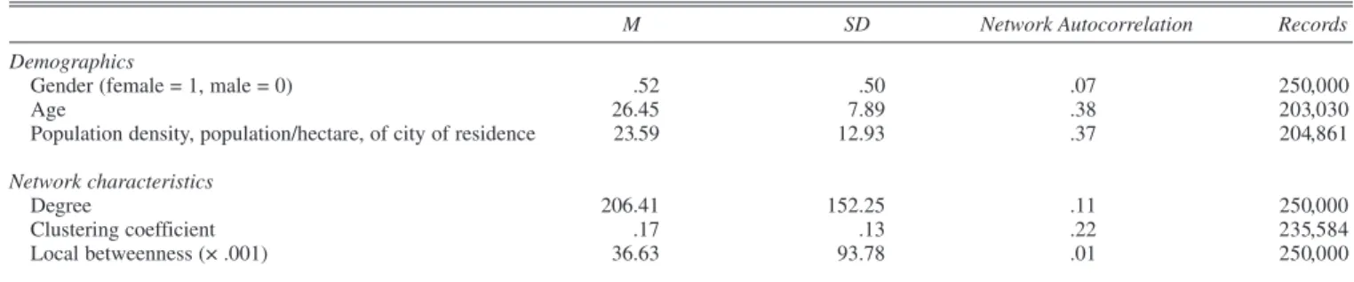
users, corresponding to a friendship density of. Table 1 sum-marizes the distributions of the demographic variables and network characteristics defined in the “Model” section.
In Table 1, we also report the correlations of demograph-ics and network characteristdemograph-ics between related actors in the network. Whereas the network characteristics of neighbors are indeed positively correlated, these weak correlations are unlikely to be the drivers of the results of our estimations. Finally, Table 2 reports correlations of the independent vari-ables used in our estimations. These correlations, together with the network autocorrelation information in Table 1, suggest that age, gender, and population density are good control variables. We note that the network autocorrelation is higher for the age and population-density variables, which suggests that we should consider group effects within age clusters and within cities. We address these estimation issues in the “Individual and Group Effects” subsection.
In the outline of the stochastic model, we defined a dis-tinguished group of people who are already using the serv-ice at the start of the analyzed period. In our empirical analysis, we include the first 2121 members in this initial group because these members received their membership directly from the creators of the social network. Finally, because the database contains registration dates for every member, we choose days to be the unit of time (thus esti-mating daily adoption probabilities in our model). Next, we present the details of the estimation.
Estimation
The estimation is based on the network-based influence model described in Equations 1 and 2. We apply the com-plementary log–log regression using the maximum likeli-hood method to obtain parameter estimates. The observa-tions we use are based on daily adoption decisions. Every day, we record the decision of each individual who has not yet adopted along with the variables described in the previ-ous section. Some of these variables are constant over time, and some of them change as the adoption process moves forward. Because we have 250,000 individuals in the data set that we analyze throughout a period of 1247 days, we obtain close to 200 million such observations. Just storing the values of our variables for all of these observations would exceed our computational capacities. To overcome this problem, we discretize some of our variables so that we could store the observations in a grouped table. For the vari-ables we discretize, we split the range of the variable into 100 equal intervals. For each interval, we only store the average value of the variable over observations that lie in the interval. In this way, we are able to reduce the space
required to store our observations (which can be represented by integer coordinates of points in a multidimensional grid) and run the maximum likelihood estimation. To examine in detail how the number of intervals chosen affects the results, we build the multidimensional grid several times, each time with randomly selected dimensions that contain only 50 equal intervals (keeping 99 ticks at the others). We find that the 95% confidence intervals overlap for the vast majority of the coefficients, which confirms the validity of this approach. Because of space limitations, we omit the exact results from this article.
Because our primary focus is on investigating how observed network characteristics can predict adoption prob-abilities, we first estimate a model (Model 1) with network effects only. Beyond these effects, Model 2 also includes influencer effects and adopter effects that are still network related, that is, have been calculated from the ultimate friendship network of the population. In Model 3 (the full model), in addition to the predictors considered in Models 1 and 2, we also include all the demographic variables. Results
Table 3 summarizes the results of the complementary log–log regressions. Across Models 1, 2, and 3, we find con-sistent support for the positive effect of degree and cluster-ing. Specifically, following the general intuition expressed in the “Measures” subsection, we observe a clear degree effect: Having more adopted neighbors increases the likeli-hood of a potential adopter to adopt, and while holding the number of adopted friends constant, having a higher total number of friends decreases adoption likelihood. More interesting is the strong support for the clustering effect. Consistent with network closure theory, a set of highly con-nected individuals has a stronger influence on a potential adopter than an identical number of sparsely connected ones. It is interesting to observe how strong the clustering effect is. When an individual has 100 friends and 6 of them have already adopted, then one extra adopted friend has the same effect on his or her adoption probability as one extra friendship between the 6 adopted friends. Finally, the inter-action of degree and clustering is also significant and posi-tive in the richer models, which provides partial support for the general intuition that the marginal effect of an additional influencer is larger for highly connected networks.
For influencer variables, we do not find significant effects for betweenness, indicating that structural hole theory may not apply to significantly large social networks in a straight-forward way. Another interesting finding is that total degree has a relatively weak but significant, negative effect, Table 1
SUMMARY STATISTICS FOR ThE STUDIED POPULATION OF NETWORK MEMBERS
M SD Network Autocorrelation Records
Demographics
Gender (female = 1, male = 0) .52 .50 .07 250,000
Age 26.45 7.89 .38 203,030
Population density, population/hectare, of city of residence 23.59 12.93 .37 204,861
Network characteristics
Degree 206.41 152.25 .11 250,000
Clustering coefficient .17 .13 .22 235,584
N e tw o rk E ffe c ts a n d P e rs o n a l I n flu e n c e s 4 3 3 Table 2
CORRELATION COEFFICIENTS OF ADOPTION DETERMINANTS
Adoption Determinant Variables
Variable X1 X2 X3 W1 W2 W3 W4 W5 Z1 Z2 Z3 Z4 Z5 Z6
Degree (X1)
Clustering (X2) –.03
Degree × clustering (X3) .67 .40
Influencer total degree (W1) –.08 .10 –.01
Influencer betweenness (W2) –.08 .00 –.04 .73
Influencer clustering (W3) .02 .16 .15 –.19 –.10
Influencer age (W4) .03 –.04 –.02 –.13 –.09 –.29
Influencer gender (W5) .08 –.03 .04 –.10 –.06 .11 –.11
Adopter total degree (Z1) –.06 –.15 –.17 .25 .03 .03 –.29 –.05
Adopter betweenness (Z2) .00 –.03 –.03 .04 .01 –.02 –.01 –.01 .38 Adopter clustering (Z3) .03 .39 .44 .01 .00 .35 –.09 .06 –.37 –.08 Age (Z4) .20 –.06 .09 –.15 –.04 –.28 .32 –.05 –.19 .00 –.13 Gender (Z5) –.02 –.02 –.03 .01 .01 .00 –.02 .19 –.01 –.02 –.01 –.08 Population density (Z6) .24 –.06 .12 .01 –.02 –.16 .05 .03 –.06 .00 –.09 .11 .03 Network size (T1) .50 –.07 .26 –.19 –.05 .30 –.11 .18 –.11 –.02 .12 –.07 .00 –.11
suggesting that individuals with many connections have less influential power on a particular neighbor.
The remaining influencer variables are all significant. The significance of the demographic variables shows that, in a practical setting, these are useful predictors for influen-tial power. For this social network site, we find that younger people and female network members have a greater influ-ence. This result is somewhat surprising because many researchers in sociology have acknowledged that men have a greater social power (Dépret, Fiske, and Taylor 1993). However, influencing adoption likelihood to a social net-work portal may be substantially different from the general notion of social power. To further examine the effects of age and gender, we estimate Model 3 separately for different genders and age groups. Besides confirming the direction and strength of the effects listed herein, we generally find greater influencer effects for similar individuals and a sig-nificantly greater influence of females among younger indi-viduals. We do not report the results of these estimations here, but in the “Individual and Group Effects” section, we
test whether such unobserved heterogeneity in the relation-ships affects the validity of our findings.
Regarding adopter effects, we also find significant results. In general, these results are consistent across mod-els except for adopter betweenness, which changes sign between Models 2 and 3. The total degree of an individual, for example, has a positive effect on his or her adoption probability; this is not surprising considering that we also included the proportion of already adopted friends in the equation, through which the total number of friends relates to the dependent variable negatively. However, an alterna-tive cause may be endogeneity, whereby the “more enthusi-astic” network users gather more friends online, which could invalidate our assumption on the exogeneity of the final network. To verify that this is not the case, we conduct several tests, which we present in the “Network Dynamics” subsection.
With respect to demographics, we find that age and popu-lation density of the town of residence both have small but significant effects, whereas gender does not. It is interesting Table 3
PARAMETER ESTIMATES OF DIFFERENT MODEL SPECIFICATIONS
Model 1: Model 2: Model 3: Model 2b: Model 3b:
Probability of Adoption M (z-Value) M (z-Value) M (z-Value) M (z-Value) M (z-Value) Network Effects Degree 4.476** 4.383** 4.476** 4.401** 4.483** (215.95) (183.41) (114.27) (182.90) (114.21) Clustering .361** .689** .704** .703** .713** (18.02) (32.48) (24.89) (33.06) (25.16) Degree × clustering –1.916** .552** 1.305** .492** 1.274** (–43.31) (7.33) (10.00) (6.50) (9.76) Influencer Effects
Average total degree –.00075** –.00090** –.00079** –.00092**
(–17.50) (–15.64) (–18.18) (–15.91)
Average (total degree)² (× .001) .000020 .000027*
(1.86) (2.27) Average betweenness (× .001) –.0067 .000025 –.000075 –.0000013 (–1.88) (.59) (–1.89) (–.03) Average clustering 3.867** 4.269** 3.777** 4.197** (28.48) (21.22) (27.70) (20.82) Average age –.0082** –.0082** (–7.24) (–7.24)
Gender (fraction of females) .076** .077**
(3.57) (3.62) Adopter Effects Total degree .0010** .0011** .0012** .0013** (39.02) (34.78) (33.57) (27.63) (Total degree)² (× .001) –.00027** –.00020** (–6.95) (–3.98) Betweenness (× .001) –.00022** –.00020** .000066 –.000016 (–7.02) (–5.44) (1.77) (–.33) Clustering –2.614** –3.322** –2.548** –3.266** (–40.86) (–34.38) (–39.52) (–33.59) Age .0029** .0030** (5.89) (6.11)
Gender (male = 0, female = 1) .0068 .0070
(.96) (.98) Population density .0012** .0012** (city of residence) (3.97) (4.06) Network size (× .001) .013** .012** .012** .012** .012** (134.39) (118.44) (92.28) (118.08) (92.18) Constant –8.830** –8.896** –8.903** –8.922** –8.925** (–1029.77) (–455.45) (–183.19) (–450.13) (–182.36) Observations 188,631,660 188,628,849 136,829,184 188,628,849 136,829,184 Pseudo-R² .0455 .0487 .0496 .0487 .0496 *p< .05. **p< .001.
Network Effects and Personal Influences 435 that age has a positive effect, which generally contradicts
empirical findings in the diffusion literature, because younger people have been shown to be generally more likely to adopt early. However, we already control for network-related variables that may cause younger users to sign up sooner if the network density is greater among them. In addition to age, we find that population density of adopters’ home city has a marginal positive effect. Note that we find this latter effect in addition to the already discussed network effects, which already capture the potentially greater density of social connections in highly populated areas.
We also conclude that adopters’ propensity to join the network increased with the overall network size, which may indicate the presence of some offline buzz about the site. However, because network size and time are almost per-fectly correlated, it is also possible that this positive coeffi-cient indicates that later network members became more accustomed to Internet technologies (in particular, the con-cept of a web-based online social network) over time and, thus, adopted with larger probability.
Comparing the fit of models, the Akaike information cri-terion (AIC), the Bayesian information cricri-terion (BIC), and McFadden’s pseudo-R-square measure all rank the models in the same order. The AIC and BIC measures require the same number of observations across estimations; therefore, we compute them over the 136,829,184 full observations included in Model 3. We list the actual values of these met-rics in Table 4. However, because we believe that consider-ing broader samples for the simpler models is more useful for interpreting the results, in most of the tables (including Table 3) we only report the pseudo-R-square values. Although Model 3 provides the best fit on the basis of all of the three measures, the corresponding pseudo-R-square value is still only .0496. The explanation for such low values is that, because the mean of our dependent variable is less than
.001, the null model makes many good predictions (by always predicting nonadoption). Thus, low fit measures do not necessarily weaken our findings. However, because the independent variables are weakly positively correlated for network neighbors (see Column 4 in Table 1), it is possible that even characteristics of the real-life friendship network are driven by unobserved similarities among network neigh-bors (Manski 1993). The finding that the coefficients of Models 2 and 3 are similar while the explanatory power of Model 3 is greater indicates that this is not the case, thus providing support for the results. Because we are not inter-ested in the formation of the final friendship network per se but rather in the diffusion on an existing network of friend-ships, we leave all further discussion of this issue to the “Robustness and Validity Tests” subsection.
Predictive Power
The results of the previous section demonstrate how local network characteristics may influence adoption likelihoods. Here, we demonstrate how our models can help predict which individuals will adopt in the near future.6Existing
models such as the Bass (1969) model perform well in fore-casting the overall number of adopters but do not provide any prediction on which individuals are more or less likely to adopt. Our methodology enables us to predict the adop-tion probabilities of individuals who have not adopted up to a certain point in time. However, it is not straightforward to measure the predictive power of our model if the outputs are probabilities, especially if these probabilities are as low as our daily adoption rates (less than .001). In real applica-tions, it is often required to predict who the next adopters will be and not only provide probability predictions. There-fore, to test the predictive power of our models, we rank-order
Table 4
COMPARINg MODEL FIT OVER ThE SAME SET OF OBSERVATIONS
Model 1: Model 2: Model 3:
Probability of Adoption M (z-Value) M (z-Value) M (z-Value)
Network Effects
Degree 4.929* (154.49) 4.535* (120.68) 4.476* (114.27)
Clustering .363* (13.51) .690* (24.47) .704* (24.89)
Degree × clustering –2.144* (–22.88) 1.312* (10.06) 1.305* (10.00)
Influencer Effects
Average total degree –.00087* (–15.57) –.00090* (–15.64)
Average betweenness (× .001) .000022 (.52) .000025 (.59)
Average clustering 4.516* (24.20) 4.269* (21.22)
Average age –.0082* (–7.24)
Gender (fraction of females) .076* (3.57)
Adopter Effects
Total degree .0011* (34.66) .0011* (34.78)
Betweenness (× .001) –.00018* (–5.22) –.00020* (–5.44)
Clustering –3.354* (–34.86) –3.322* (–34.38)
Age .0029* (5.89)
Gender (male = 0, female = 1) .0068 (.96)
Population density (city of residence) .0012* (3.97)
Network size (× .001) .013* (106.69) .012* (94.59) .012* (92.28) Constant –8.830* (–845.80) –8.981* (–367.65) –8.903* (–183.19) Observations 136,829,184 136,829,184 136,829,184 Pseudo-R² .0461 .0495 .0496 AIC 1,368,561.20 1,363,723.66 1,363,624.20 BIC 1,368,644.87 1,363,907.74 1,363,891.95 *p< .001.
the individuals in decreasing adoption likelihood and com-pare the top m individuals of this list with the set of the next m individuals who adopted in reality. We do this for differ-ent values of m; to determine the number m to be used in the context of a real application, one could, for example, use an aggregate-level model to predict the number of individuals adopting in the next period under consideration.
Because our adoption data are distorted after the studied period for previously mentioned reasons, we make predictions for the last ten days before the cutoff point, day 1247.7
There-fore, we first estimate our models on the first 1237 days of the adoption data. Next, using the resulting coefficients and the total network data, we calculate the predicted probability of adoption for each individual on day 1238. Then, we rank these predicted probabilities and list the nodes to which the m high-est probabilities belong as a prediction for the next m adopters. Let M denote the set of these individuals with |M| = m.
We test the predictive power of four models. The first three are the same three main models we used in the “Esti-mation” subsection. Model 4 is a benchmark in which we ignore the network variables and include only demographics and network size. We drop all observations for which any of the variables used in any of the models are missing. To test predictive power, we calculate what percentage of individu-als in M really adopted during the ten-day period. Table 5 shows the results for different values of m.
The highest value we use, m = 9944, is the actual number of adopters during this period, which constitutes 11.66% of the potential adopters in our sample. Thus, a random set of size 9944 would have a hit rate of 11.66%. We use this as a benchmark, in addition to the prediction based on only the available demographic variables (Model 4), which success-fully predicts 13.25% of the adopters. Using any of our three main models, we can almost double the hit rate from the ran-dom benchmark to approximately 21%, substantially improving the predictive power over that of Model 4. Dis-playing the success rates for Models 3 and 4 as a function of m, Figure 4 shows this pattern. As Table 5 shows, Models 1 and 2 yield results similar to those of Model 3. If the appli-cation only requires the identifiappli-cation of a lower number of adopters than the total expected number of adopters, then the hit rate becomes even higher. For values around m = 500, Models 1, 2, and 3 predict adoption successfully with an approximate 30% probability. That is, for applications for which not only successful predictions are of interest but also
the cost of “false-positive” predictions is somewhat larger, it may be best to focus on only approximately 5%–10% of future adopters. In such scenarios, our model performs much better than the random selection (11.66% success rate) and the model based solely on demographic variables (13.60% success).
Robustness and Validity Tests
In this section, we address several limitations of our model, data, and estimation procedure. We begin by allowing for latent individual heterogeneity in the propensity to adopt. Because of the computational limitations discussed in the “Estimation” subsection, we are only able to estimate such models on a smaller (random) sample of individuals. In a dif-ferent approach, we implode the friendship network into net-work layers containing only relationships within the same city of residence to examine whether our results still hold within these networks to garner further support for our sub-stantive findings. We continue by considering alternative model formulations. We change the link function, and we test an alternative definition of our main independent variable. Third, we discuss a number of issues related to network dynamics. By eliminating certain individuals, links, and deci-sions from our data set, we challenge our assumption on the exogeneity of the real-life friendship network and explore the potential effects of heterogeneous link strength on our results.
Figure 4
PROPORTION OF ADOPTERS AMONg PREDICTED OUT-OF-CALIBRATION SAMPLE ADOPTERS AS A FUNCTION OF ThE SIZE OF ThE PREDICTION LIST
Table 5
ADOPTION PERCENTAgE OF PREDICTED ADOPTERS
Successful Prediction Rate (%)
Number of Adopters Predicted (m) Model 1 Model 2 Model 3 Model 4 Random
500 30.60 29.60 28.80 13.60 11.66
1000 26.80 27.60 27.20 13.40 11.66
2000 24.45 24.45 24.40 12.35 11.66
4000 23.15 23.32 23.22 12.10 11.66
9944 20.71 21.19 21.19 13.25 11.66
7The prediction process does not depend on the number of days, and the predicted sets would be the same for different periods. However, the actual probabilities would be small for one day, and it is more realistic to consider a longer period.
Network Effects and Personal Influences 437 Individual and group effects. In this section, we carry out
tests to verify the validity of the assumption on the inde-pendence of the error terms in our main models. First, we estimate our model including random effects:
(5)
where we assume that uv~N(0, s2). Because the random
effects vary according to individual, we have to break with our estimation method of discretizing the independent vari-ables, which assumes homogeneity within each cell in the grid (which may contain observations from different individ-uals). Thus, to run the random-effects model on the whole adoption data set, we would have to deal with well over 100 million observations. Because this is clearly infeasible, we randomly select 5000 individuals from the 250,000 network members and run the random-effects estimation on the data comprised of observations concerning only these individu-als. (However, we compute the independent variables from the network spanning over all the individuals in the data.) We present the results of this process in Table 6. The large value of r confirms that the low model fit measures reported in Table 3 may indicate unobserved heterogeneity in the rela-tionships. Nevertheless, although the coefficients cannot be directly compared with those in Table 3, we find that most of the effects identified by our main estimation are sup-ported by the results herein as well. The finding that some of the demographic variables become insignificant suggests that demographics may be correlated with the unobserved propensity of adoption, which we capture here by individ-ual random coefficients. Finally, our choice of restricting the structure of individual effects to the normal distribution is a result of computational limitations: The data sample that
f(S, v) = 1 X (S) + W(S) Z(v) + v − − + × × + × exp{ exp[α β γ ϕ uv]},
we consider contains several million observations per regression, which makes estimating 5000 fixed-effect dum-mies infeasible.
Next, we return to our original model formulation (with-out individual effects), but we allow the error terms to be correlated for homogeneous age or gender groups to arrive at more robust standard-error estimates. In general, we find that the network effects we examine remain significant. In Table 7, we present a specific example leading to the largest decrease in the strength of the effects that we obtain this way. For this estimation, we divide the population into five age clusters (21, 22–23, 24–26, 27–29, and 30). The parame-ter significances corresponding to the robust standard error estimates provide further support for the degree and cluster-ing effects and also for the negative effect of influencer total degree. However, the degree–clustering interaction and betweenness do not have significant effects under these cir-cumstances.
Finally, to explore the validity of some of our substantive findings, we refine the personal networks by dedicating spe-cial attention to friendships within the same city of resi-dence. We split all network variables except clustering. We jointly estimate the impact of the number of friends from the same city and the impact of the number of friends from other towns. In a similar way, the average betweenness of network neighbors from the same city and the average of those from other towns become two independent variables. (In the case of the clustering variable, we do not have a straightforward way to do the same, because across-town friendships in one’s personal network may be present. Thus, clustering may not arise as a sum of within-city and across-cities components.) For the degree–clustering interaction, we have two choices: In Model 5, we include the degree variable as before (referring to the proportion of adopted friends), and in Model 6, we include the within-city degree Table 6
PARAMETER ESTIMATES: RANDOM-EFFECTS COMPLEMENTARY LOg–LOg REgRESSION
Model 1: Model 2: Model 3:
Probability of Adoption M (z-Value) M (z-Value) M (z-Value)
Network Effects
Degree 31.144** (59.23) 36.963** (36.60) 35.655** (28.82)
Clustering 1.275* (3.41) 3.013* (3.47) 1.400* (2.84)
Degree × clustering –13.635** (–10.90) 24.959** (4.23) 25.448** (5.46)
Influencer Effects
Average total degree –.012** (–9.67) –.011** (–7.38)
Average betweenness (× .001) .0054** (7.35) .0040** (6.81)
Average clustering 31.374** (6.33) 23.383** (4.69)
Average age .012 (.59)
Gender (fraction of females) .145 (.34)
Adopter Effects
Total degree .0088** (4.48) .0081** (4.91)
Betweenness (× .001) .0034 (.52) .0064 (1.66)
Clustering –32.318** (–13.60) –33.609** (–12.46)
Age .027 (.96)
Gender (male = 0, female = 1) .067 (.27)
Population density (city of residence) .0054 (.52)
Network size (× .001) .079** (45.93) .067** (39.30) .088** (28.52) Constant –21.543** (–99.44) –22.411** (–36.41) –24.331** (–17.02) Observations 3,780,234 3,772,389 2,730,623 Individuals 4594 4552 3208 r .9741 .9653 .9825 *p< .01. **p< .001.
(proportion of adopted friends considering only within-city friendships).
In Table 8, we show the coefficient estimates of Models 5 and 6. We find support for the degree and clustering effects as well as the negative effect of influencer total degree. The degree–clustering interaction is only supported in Model 6, and we cannot detect the positive effect of betweenness (that structural hole theory would predict). An interesting phenomenon is the effect of network size: Despite all the within-city network variables being more significant than their across-cities pairs, the opposite is true for network size, and the coefficient of within-city network size is nega-tive. This suggests that the positive coefficient of network size in Models 1–3 indicates the evolution of users’ affinity for technology rather than the presence of offline buzz.
Alternative model formulations. In this section, we dis-cuss the most straightforward alternatives to some of our modeling choices. We begin by including two quadratic terms in our models to determine if the negative effect of influencer total degree is driven by actors with signifi-cantly large personal networks. As the results (see Columns 5 and 6 of Table 3) indicate, the square of influ-encer total degree is not or is only marginally significant, and it has a positive coefficient. This result suggests that our main results are not driven by highly connected indi-viduals and that they hold for actors with smaller personal networks as well.
Next, we change our main independent variable from the proportion of already adopted friends within all friends of adopters to their number. Table 9 lists the estimates of the model. Although we find that all major results are consis-tent with those presented in Table 3, we also note that the model fit values are lower for this alternative specification. In summary, the proportion, not the sheer number, of
already adopted friends explains more about the adoption decisions studied.8
Finally, we replace the complementary log–log link func-tion (Equafunc-tion 2) with the logit funcfunc-tion and reestimate our original models. Because all coefficients and z-values are similar to the results of the complementary log–log regres-sion, we do not report the results herein.
Network dynamics. Throughout this work, we have relied on the assumption that the observed network at the time of the study is final and static in the sense that we can observe all the real-life friendships among individuals in the network; this is inaccurate for two related reasons. On the one hand, numerous friendships appearing in the data could have been made during the 3.5 years we analyze. On the other hand, there were probably some existing real-life friendships not confirmed in the network before the friendship data were col-lected. If the observed final network data are not a good proxy for the structure existing in real-life friendships, our results may be biased. In that case, it could be argued that individu-als who had spent less time as users (i.e., people joining the network later) might not have enough time to map out all their friends present in the network. Then, the independent variables for these people (i.e., their network characteristics) might be erroneous. Similarly, being a member of the service to make more friends might be a typical user behavior. In such a case, members with many friends would have a greater propensity to make new friends. In this case, the rate of the 8An interesting difference between the estimates of the two models is the coefficient of Adopter Total Degree. Goldenberg et al. (2009) propose that social hubs tend to adopt earlier because of more exposure to the prod-uct in question. In Table 9, the number of (possible) exposures is directly captured in the Network Degree variable. Because the coefficient of Adopter Total Degree is negative in this estimation, we indeed find empiri-cal support for the explanation of hubs’ early adoption.
Table 7
PARAMETER ESTIMATES: CORRECTINg FOR UNOBSERVED hETEROgENEITY
Model 1: Model 2: Model 3:
Probability of Adoption M (z-Value) M (z-Value) M (z-Value)
Network Effects
Degree 4.476*** (10.01) 4.383*** (11.54) 4.476*** (12.53)
Clustering .361*** (7.43) .689*** (25.18) .704*** (70.19)
Degree × clustering –1.916*** (–5.06) .552** (2.68) 1.305 (1.69)
Influencer Effects
Average total degree –.00075** (–3.40) –.00090*** (–5.53)
Average betweenness (× .001) –.0067 (–1.86) .000025 (.66)
Average clustering 3.867*** (11.31) 4.269*** (9.04)
Average age –.0082* (–2.39)
Gender (fraction of females) .076 (1.91)
Adopter Effects
Total degree .0010*** (10.35) .0011*** (20.11)
Betweenness (× .001) –.00022*** (–8.89) –.00020*** (–3.72)
Clustering –2.614*** (–13.30) –3.322*** (–6.28)
Age .0029 (.76)
Gender (male = 0, female = 1) .0068 (.26)
Population density (city of residence) .0012** (3.28)
Network size (× .001) .013*** (4.19) .012*** (4.20) .012*** (4.91) Constant –8.830*** (–27.25) –8.896*** (–31.45) –8.903*** (–25.46) Observations 188,631,660 188,628,849 136,829,184 Pseudo-R² .0455 .0487 .0496 *p< .05. **p< .01. ***p< .001.