A novel semi-supervised convolutional neural network method for synthetic aperture radar image recognition

*Corresponding Author, E-mail: [email protected], Tel: +86-010-82317240, Fax: +86-010-82317240 1 _{School of Electronic Information Engineering, Beihang University, Beijing 100191, China}

2 _{Strathclyde Space Institute, Department of Design, Manufacture and Engineering Management, University of}

A Semi-Supervised CNN Method for SAR Image Recognition

Zhenyu Yue1_{, Fei Gao}1*_{, Qingxu Xiong}1_{, Jun Wang}1_{, Teng Huang}1_{, Erfu Yang}2_{, Huiyu Zhou}3

Abstract

Background / introduction: SAR image automatic target recognition technology (SAR-ATR) is one of the research hotspots in the field of image cognitive learning. Inspired by the human

cognitive process, experts have designed convolutional neural networks (CNN) based methods

and successfully applied the methods to SAR-ATR. However, the performance of CNNs

significantly deteriorates when the labelled samples are insufficient.

Methods: To effectively utilize the unlabelled samples, a semi-supervised CNN method is proposed in this paper. First, CNN is used to extract the features of the samples, and subsequently

the class probabilities of the unlabelled samples are computed using the softmax function. To

improve the effectiveness of the unlabelled samples, we remove possible noise performing

thresholding on the class probabilities. Afterwards, based on the remaining class probabilities, the

information contained in the unlabelled samples is integrated with the scatter matrices of the standard linear discriminant analysis (LDA) method. The loss function of CNN consists of a

supervised component and an unsupervised component, where the supervised component is

created using the cross-entropy function and the unsupervised component is created using the

scatter matrices. The class probabilities are utilized to control the impact of the unlabelled samples

in the training process, and the reliability of the unlabelled samples is further improved.

Results: We choose ten types of targets from the Moving and Stationary Target Acquisition and Recognition (MSTAR) dataset. The experimental results show that the recognition accuracy of

our method is significantly higher than that of the supervised CNN method.

Conclusions: It proves that our method can effectively improve the SAR-ATR accuracy despite the deficiency of the labelled samples.

Key words:

1.

Introduction

Synthetic Aperture Radar (SAR) has been widely used due to its high resolution and

penetrating ability [1-3]. SAR image automatic target recognition technology (SAR-ATR) is one

of the research hotspots in the field of image cognitive learning [4,5]. Based on the cognitive system, humans are able to recognize targets quickly and accurately. Inspired by this, various

methods that imitate the human cognitive system have been proposed to improve the SAR-ATR

accuracy.

The image cognitive system of humans is based on neural networks [6]. Image signals

acquired by the retina first go through the primary visual cortex for extracting edge and orientation features, followed by the generation of shape and contour features. In this way, image signals pass

through the higher level visual cortex and we can obtain the more abstract features. Hence, human

image cognition is a process of obtaining abstract features through layer-by-layer visual cortex

[7,8]. Inspired by this process, people have established various neural network models. By

simulating the whole process of the human vision system from the retina to the visual cortex, an

effective SAR image feature extraction method was proposed in [9]. Using the hierarchical perceptual inference process embedded in the cortex, Spratling et al proposed a hierarchical neural

3

network (CNN) based on the human visual system (HVS) [11]. CNN simulates the visual cortex

using convolution layers and each convolution layer contains several convolution kernels for

extracting abstract features of the image data. Compared with the other neural network models,

CNN has been successfully applied to SAR-ATR due to its powerful feature extraction capability [12-14].

Chen et al. designed a CNN model with a single layer to automatically extract features for

SAR target recognition [15]. SAR images are transformed into a set of feature maps after certain

convolution and pooling operation. Subsequently, the feature maps are used to train the softmax

classifier. Gao et al. proposed a new SAR-ATR method by combining CNN and Support Vector Machine (SVM) [16]. The experimental results prove that the proposed method can achieve an

average accuracy of 99% on ten types of targets. However, the CNN model needs a large number

of labelled samples in the training process. When the labelled samples are insufficient, the

recognition accuracy of the CNN decreases significantly [17]. Because of the imaging nature,

speckle noise and clutters exist in SAR images and the outline of the targets is weak, which increases the difficulty of the sample annotation. As a result, the number of the labelled samples is

insufficient, which restricts the application of CNN in SAR-ATR. In recent years, researches have

focused on improving the SAR-ATR’s accuracy with a small labelled dataset. In [18], the center

loss is adopted and combined with the softmax loss to train the deep CNN. However, compared

with labelled samples, unlabelled samples are easy to acquire. Besides, unlabelled samples also

contain a wealth of information which helps to improve the SAR-ATR’s accuracy.

Human cognition does not need a large number of labelled samples, Inspired by this

accuracy when the labelled samples are insufficient [22,23]. The commonly used semi-supervised

learning methods include self-training, co-training, graph-based methods, and semi-supervised

support vector machines [24-26]. Lv et al. proposed a semi-supervised predictive sparse

decomposition method for feature learning [27]. To solve the online semi-supervised learning problems, Ding et al. proposed a novel manifold regularized model in a reproducing kernel Hilbert

space [28].

Recently, researchers are focusing on combining semi-supervised learning methods with

neural network models. To effectively utilize the unlabelled samples, a semi-supervised deep

learning model based on ladder networks was proposed in [29]. Consisting of a corrupted encoder, a clean encoder and a decoder, the proposed model is trained to minimize the sum of the

supervised loss function and the unsupervised loss function. Samuli and Timo proposed two

simple and efficient semi-supervised CNN models, i.e. the Pi and the temporal ensembling models

[30]. The two models are based on the self-ensembling method, where the predicted labels of the

unlabelled samples are generated using the output of CNN at different epochs. According to the predicted labels, the unlabelled components of the loss function are obtained. The experimental

results show that the two models improve the image recognition accuracy greatly when the

labelled samples are insufficient. Although the above semi-supervised methods are proved to be

effective, it is found that semi-supervised methods cannot always improve the image recognition

accuracy because of the noise and interference in the unlabelled samples [31,32]. For example, the

Pi and the temporal ensembling models use CNN to predict the labels of the unlabelled samples. However, the reliability of the unlabelled samples is significantly reduced if the predicted labels

5

unlabelled samples restricts the application of semi-supervised methods in image recognition.

In this paper, a new semi-supervised CNN method is proposed to improve the SAR-ATR

accuracy when the labelled samples are insufficient. First, CNN is used to extract the features of

the samples, and the class probabilities of the unlabelled samples are obtained using the softmax function. In order to improve the reliability of the unlabelled samples, we perform thresholding

processing on the class probabilities. Afterwards, based on the class probabilities, the information

contained in the unlabelled samples is integrated with the scatter matrices of the standard LDA

method. The loss function of CNN consists of a supervised and an unsupervised component. The

supervised component is created by the cross-entropy function and the unsupervised component is created using the scatter matrices. The class probabilities are utilized to control the impact of the

unlabelled samples in the training process, and the reliability of the unlabelled samples can be

further improved.

The rest of this paper is arranged as follows. In section 2, CNN and the LDA methods are

briefly introduced. Section 3 describes the principle of our proposed method in detail. The experiments based on the MSTAR database are performed in Section 4. Finally, we summarize our

contribution in section 5.

2.

Preliminary

2.1 Convolutional Neural Network

CNN is mainly composed of convolution, pooling and fully connected layers. The

convolution layers are used to extract image features. The pooling layers decrease the risk of overfitting by reducing the number of features, and the fully connected layers are used to integrate

[33,34].

In the forward propagation process, the current layer of CNN receives the output of the

previous layer, which is expressed as follows: 1 ( ) l l l l l l z w a b a  z  _  _{ }   _ （1） where l denotes the lth layer. zl, wl and bl represent the weighted input of the lth layer,

the weight matrix and the bias matrix, respectively.



andalrepresents the actual output value of the lth layer. If l1, a0 represents the pixel value of the input image.

In the backpropagation process, the parameters wl and bl of CNN are updated using the

back propagation (BP) algorithm. In detail, the BP algorithm firstly constructs a loss function

based on the actual and the expected output of CNN. Afterwards, the gradient descent method is

utilized to update the parameters wl and bl along the gradient decent direction of the loss

function. Suppose that E₀ is the loss function and L denotes the number of the layers of CNN,

the error vector of the output layer is expressed as follows: 0 L L E z    （2） The error vector of the (l1)th layer can be calculated from the error vector of the _lth _layer.

Therefore, the error vector l of each layer can be calculated by the Chain Rule:

1 1 ' ( ) l l l l w z







where the symbolicorepresents the element-wise product of the two vectors. The partial

derivative of E0 to l

7 1 0 0 0 0 l l l l l l l l l l l E E z a w z w E E z b z b                 _  _       o o o （4）

Then, the change values of wl and bl are calculated:

0 0 l l l l E w w E b b        _    _    _   （5）

Where  denotes the learning rate.

2.2 Linear Discriminant Analysis (LDA)

LDA is used to search a subspace where the samples of different classes are distant from each

other while the samples of the same class are close to each other [35,36]. In case of binary

classification, given the training dataset









1

, m

i i _i

D x y _ , wherex_idenotes the training samples

and yi

 

training dataset. Suppose that _i and C_i represent the mean vector and covariance matrices of

the ith class respectively, and w denotes the projection vector. In order to make the samples of

the same class as close as possible in the subspace, 0 1

T T

w C w w C w should be small. While 2

0 1 ₂

T T

w  w  should be large to make the samples of different classes as distant as possible. Thus, taking these into consideration, we get the optimization objective function as follows.











Then we define the within-class scatter matrix S_wC₀C₁ and the between-class scatter matrix







T b

S      . Then the objective function Eq. (6) can be rewritten as Eq. (7), which is

called the “generalized Rayleigh quotient” of S_w and S_b.

T b T w w S w J w S w  （7）

Next, the LDA algorithm is extended to the field of multi-classification. Suppose that there are N

classes and the number of the samples of the ith class is m_i. First, the total-class scatter matrix

is defined as follows,









where m denotes the total number of the samples and  represents the mean vector of all the

samples. The within-class scatter matrix is defined as the sum of the covariance matrices for each class: 1 N w i i S C  



According to Eqs. (8) and (9), the between-class scatter matrix is obtained:









There are various ways to construct the optimization objective function of LDA for

multi-classification, and one of the common ways is expressed in Eq. (7).

3.

The proposed method

First, we define the system parameters. The training dataset consists of two parts:

[ , ] d N

X L U R  , where [ ,1 2, , ]

d l l

L x x L x R  represents the labelled dataset and

1 2

[ l , l , , l u] d u

U  x_ x_ L x_ R  represents the unlabelled dataset. d denotes the dimension of the

9

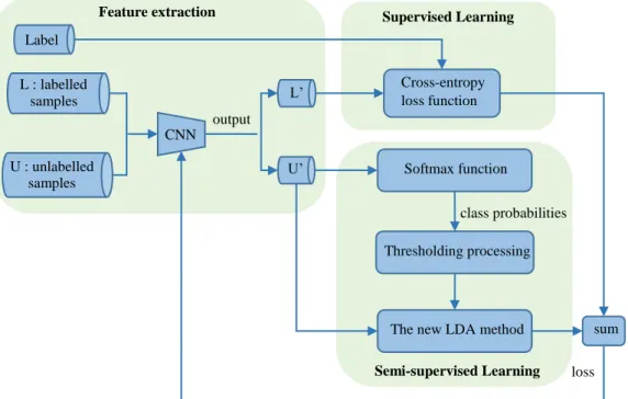
Figure 1: The flowchart of the training process

As shown in Figure 1, the training process of our method is composed of three parts: feature

extraction, supervised learning and semi-supervised learning. In the feature extraction, we use CNN to extract the features of the samples. L' and U' represent the feature vector of the

labelled and unlabelled datasets respectively. In the process of supervised learning, the labelled

samples are utilized to obtain the supervised component of the loss function for CNN. The

semi-supervised learning process which consists of two steps is the core of our method. First, we

calculate the class probabilities of the unlabelled samples using the softmax function. To improve

the reliability of the unlabelled samples, we perform thresholding processing on the class probabilities. Afterwards, based on the class probabilities, the information contained in the

unlabelled samples is integrated to the scatter matrices of the standard LDA method, and the

unsupervised component of the loss function is constructed using the scatter matrices. Next, the

two steps of the semi-supervised learning process are analyzed in detail.

3.1 Class probabilities of unlabelled samples

Softmax function L’ U’ CNN Feature extraction Semi-supervised Learning Cross-entropy loss function Supervised Learning L : labelled samples U : unlabelled samples Label Thresholding processing

The new LDA method class probabilities

sum loss output

To effectively utilize the unlabelled samples, we calculate the class probabilities at first.

Since the samples in L and U are high-dimensional, we use CNN to extract the features so as

to obtain the class probabilities. Compared with optical images, the signal to noise ratio (SNR)

and resolutions of SAR images are relatively low. Therefore, CNN models such as AlexNet and VGGNet for optical images are not suitable for SAR images. As shown in Figure 2, we designed

the CNN model for SAR images based on comprehensive experiments. The size of the input

images is 64*64. Conv1, Conv2 and Conv3 represent the convolution layers. The number of the

convolution kernels in Conv1 is 20, and the kernel size is 3*3. The number of the convolution

kernels in Conv2 is 40, and the kernel size is 4*4. The number of the convolution kernels in Conv3 is 80, and the kernel size is 3*3. We adopt the Relu activation function in the convolution

layers. Maxpool denotes the maximum pooling operation, and the pool size is 2*2. The Flatten

layer stretches the output of Conv3 to create a 2880 dimensional column vector. Linear1, Linear2

and Linear3 represent the fully connected layers. The output dimensions of each layer are 2880,

2880 and 10 respectively. The Relu activation function is also adopted in the fully connected layers.

11

Figure 2: The CNN model employed in the proposed method.

Suppose that the number of the neurons in the output layer is K, that is, the CNN eventually

divides the input images into K classes. As expressed in Eq. (11), we utilize the softmax function

to normalize the output of CNN, and the class probabilities of the unlabelled samples are obtained.

1 k j a k K a j e p e  



th

k class. The larger the value of pk, the greater the probability that the sample belongs to the

th k class. 1 1 K k k p  



The reliability of a sample is related to the probability that belongs to the class corresponding

to its true label. We define the reliability factor (RF) to measure the reliability of samples. As

expressed in equation Eq. (12), p_true denotes the probability of a sample belonging to the class

Input image 64*64

Conv1(20*3*3 /Relu /Maxpool 2*2)

Conv2(40*4*4 /Relu /Maxpool 2*2)

Conv3(80*3*3 /Relu /Maxpool 2*2) Flatten(2880)

Linear1(2880 /Relu) Linear2(2880 /Relu)

that corresponding to its true label. The larger the value of RF, the more reliable of a sample. In

general, a sample with the RF value greater than 0.9 can be regarded as a reliable sample.

1 true K k k p RF p  



Suppose that piR1N denotes the class probabilities of all the unlabelled samples belonging to the ith class. To improve the reliability of the unlabelled samples, we apply

thresholding processing to pi:









p represents the jth element of pi and t is the threshold. The greater the value of

t, the higher the reliability requirement for the unlabelled samples. If the maximum class

probability of a sample is less than t, all the class probabilities of the sample will be set to 0. We

utilize the unlabelled samples based on the class probabilities and the new LDA method. Thus, the

unlabelled samples whose class probabilities are all set to 0 will not be utilized in the training

process.

3.2 The new LDA method

After obtaining the class probabilities, how to effectively utilize the unlabelled samples is the

key to improving the recognition accuracy of the CNN model. Most of the semi-supervised CNN

methods extend the labelled dataset by using CNN to label the unlabelled samples. And the CNN

is retrained using the extended dataset subsequently. However, when the initial labelled samples are insufficient, the generalization ability of the CNN model is weak. As a result, the “pseudo labels” for the unlabelled samples are not credible, which restricts the improvement of the recognition accuracy. In contrast, the LDA method constructs an optimization function based on

13

the within-class and between-class distance of the samples. Using the projection vector, the

samples of different classes are distant from each other while the samples of the same class are

close to each other. Here, we design a new LDA method to exploit the unlabelled samples. In our

method, the information contained in the unlabelled samples is integrated to the scatter matrices of the standard LDA method based on the class probabilities. Then the unsupervised component of

the loss function is calculated using the scatter matrices.

In the standard LDA method, if we map the samples to a space and assume that the density of

each sample is 1. Then the mean vectors is used to denote the center of each class. We redefine the

within-class mean vector u_i and the total mean vector u in the new LDA method:

± ° 1 1 1 1 1 1 1 1 1 1 / / N i j j _N j i i i i N j j i j j j K N i j j _{K K N} i j i i j K N i i i j j i j p x u X p p X p p p x u X p p X p p               _     _                  









 



Compared with the standard LDA method, we use the class probabilities as the density of the unlabelled samples. The larger the probability of a sample belonging to a class, the greater the

impact on the class center. Since the information contained in the unlabelled samples is effectively

utilized, the mean vectors are more reliable.

Afterwards, we define the new scatter matrices:

± ° ± ° 1 1 ( )( ) [ ( )( ) ] K T b i i i i K i i T T i i T b S m u u u u X m p p p p X X S X         







± ± 1 1 1 1 ( )( ) [ ( )( ) ] k N i T w j j i j i i j k N i i i i i T T j j j i j T w S p x u x u X p h p h p X X S X           









between-class scatter matrix. In addition, the class probability pi_j is added as the weight

coefficient in the within-class and total-class scatter matrices. The greater the class probabilities of the unlabelled samples, the greater the impact on the scatter matrices. The new LDA method

controls the impact of the unlabelled samples through the class probabilities. Thus, the reliability

of the unlabelled samples is improved.

When constructing the “generalized Rayleigh quotient” optimization function, we can use

any two scatter matrices, and one of the common ways is expressed in Eq. (19). T w T b W S W J W S W  （19）

where W (w w₁, ₂,L,w_K) denotes the projection matrix. Since both the numerator and denominator of Eq. (19) are matrices, the optimization function cannot be optimized as a scalar function. Therefore, an alternative optimization function is adopted:

T K i b i T w S w J w S w _



15

According to the nature of the “generalized Rayleigh quotient”, the minimum value of J is the

minimum eigenvalue of S S_w1 _b. Afterwards, the unsupervised component of the loss function for

CNN is obtained, as shown in Eq. (21).

1 min(J ) min[eig S S( w b)]

 _ 

（21） Because of the simplicity and convergence rate of the cross-entropy function, we utilize it to

construct the supervised component of the loss function for CNN, as shown in Eq. (22).

0 1 ln (1 ) ln(1 ) k k k k x K E y a y a N  



Where ( ,y y_{1 2},L,yK) represents the expected output of CNN and ( ,a a1 2,L,aK) denotes the actual output. Based on Eqs. (21) and (22), the loss function of CNN is the sum of the two components: 1 1 [ _kln _k (1 _k) ln(1 _k)] min[ ( _{w b})] x K E y a y a eig S S N   



After the training process has been achieved, the test samples are the input of the CNN model,

and the predicted labels are obtained.

4.

Experiments

The experiments consist of two parts. First, we discuss the effectiveness of the relevant steps

in our method. Then we compare the performance of our method with that of the other

semi-supervised methods. The experiments are performed on the Moving and Stationary Target

Acquisition and Recognition (MSTAR) dataset which contains multiple types of targets. In our

experiments, we choose ten types of targets, namely, 2S1, ZSU234, BRDM2, BTR60, BMP2,

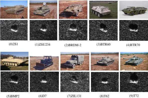
BTR70, D7, ZIL131, T62 and T72. Figure 3 shows the SAR and optical images of each type. Although the optical images are distinct from each other, the corresponding SAR images are

the training and testing datasets. The detailed information is listed in Table 1.

Figure 3: The SAR and optical images of ten types of targets in the MSTAR dataset. Table 1: The training and testing datasets of our experiment.

Type Tops Model

Training set Testing set

Depression Number Depression Number

2S1 Artillery B_01 17° 299 15° 274 ZSU234 D_08 17° 299 15° 274 BRDM2 Truck E_71 17° 298 15° 274 BTR60 K10YT_7532 17° 256 15° 195 BMP2 SN_9563 17° 233 15° 195 BTR70 C_71 17° 233 15° 196 D7 92V_13015 17° 299 15° 274 ZIL131 E_12 17° 299 15° 274 T62 Tank A_51 17° 299 15° 273 T72 #A64 17° 232 15° 196 Sum:2747 Sum:2425

4.1 Evaluation of our method

4.1.1 Evaluation of the new LDA method

In our method, a new LDA method is designed to utilize the unlabelled samples. First, in (0)2S1

(5)BMP2

(2)BRDM-2 (3)BTR60 (4)BTR70

(6)D7 (7)ZIL131 (8)T62 (9)T72

17

and the Kappa coefficients of our method with those of the supervised CNN method which only

utilizes the labelled samples. The overall accuracy refers to the ratio of the number of correctly

recognized samples to the number of all the samples. The calculation of Kappa coefficient is based

on the confusion matrix, which can well represent the recognition accuracy of each class. The definition of Kappa coefficient is shown in Eq. (24), where p_o is the relative observed

agreement between the recognition results for the test data and the real labels, and p_e represents

the hypothetical probability of the chance agreement.

1 o e e p p k p    (24) In the experiments, the training dataset is divided into a labelled dataset L and an

unlabelled dataset U. During the partition, we randomly select the same number of the samples

from each class in the training dataset, and L consists of the selected samples. U consists of the remaining samples in the training dataset. We design six different partitions and the

corresponding numbers of the samples in L and U are shown in Table 2. The Adam optimizer

is adopted when we train the CNN, and the parameters are set experimentally as follows: 0.001

 , ₁0.9, ₂0.99. When performing the thresholding processing on the class

probabilities, the value of t is set to 0.2. We repeated the experiments under different partitions

for ten times and the average results are shown in Table 3.

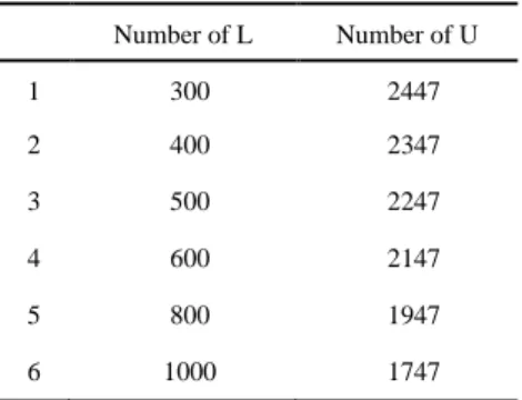
Table 2: Six different partitions of the training dataset and the corresponding numbers of samples in L and U.

Number of L Number of U 1 300 2447 2 400 2347 3 500 2247 4 600 2147 5 800 1947 6 1000 1747

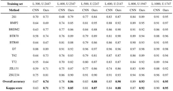
Table 3: The performance of the supervised CNN method and our method under different partitions of the training dataset. The supervised CNN method only utilizes the labelled samples while our method utilize both the labelled and unlabelled samples.

Training set L:300, U:2447 L:400, U:2347 L:500, U:2247 L:600, U:2147 L:800, U:1947 L:1000, U:1747

Method CNN Ours CNN Ours CNN Ours CNN Ours CNN Ours CNN Ours

2S1 0.70 0.73 0.68 0.79 0.77 0.84 0.83 0.87 0.84 0.89 0.91 0.95 BMP2 0.64 0.69 0.74 0.85 0.81 0.95 0.88 0.92 0.89 0.95 0.91 0.97 BRDM2 0.63 0.77 0.77 0.86 0.84 0.88 0.86 0.90 0.91 0.92 0.86 0.95 BTR70 0.58 0.74 0.76 0.89 0.79 0.89 0.81 0.90 0.89 0.94 0.88 0.96 BTR60 0.64 0.67 0.81 0.88 0.79 0.86 0.86 0.87 0.90 0.93 0.91 0.95 D7 0.88 0.89 0.91 0.92 0.96 0.97 0.96 0.96 0.97 0.98 0.99 0.98 T62 0.64 0.73 0.76 0.83 0.79 0.81 0.87 0.87 0.86 0.89 0.91 0.94 T72 0.55 0.64 0.70 0.82 0.80 0.87 0.83 0.87 0.84 0.92 0.89 0.94 ZIL131 0.59 0.71 0.75 0.87 0.77 0.86 0.74 0.86 0.83 0.90 0.88 0.92 ZSU234 0.75 0.81 0.86 0.90 0.91 0.90 0.91 0.93 0.94 0.96 0.96 0.97 Overall accuracy 0.67 0.74 0.78 0.86 0.83 0.88 0.85 0.90 0.89 0.93 0.91 0.95 Kappa score 0.63 0.71 0.75 0.85 0.81 0.87 0.84 0.88 0.87 0.92 0.90 0.95 As can be seen, the overall accuracy and the Kappa coefficients of our method outperforms

those of the supervised CNN method. The fewer the labelled samples, the more significant the

difference of the performance. And the difference gradually decreases as the number of the

labelled samples increases. The reason is that, compared with the supervised CNN method, our method utilizes the unlabelled samples effectively. As a result, the generalization ability of our

method is enhanced and the overall accuracy and the Kappa coefficients are improved. With the

increasing labelled samples, the generalization ability of the CNN model is gradually augmented,

hence the performance difference between the two methods decreases.

Next, we illustrate the effectiveness of the new LDA method. We extract the 1×10 feature

vectors of the testing samples from the output of our method and the supervised CNN method.

19

training dataset shown in Table 2 to train the two methods. The supervised CNN method only

utilizes the labelled samples while our method utilize both the labelled and unlabelled samples.

The distribution of the feature vectors from the output of our method and the supervised CNN

method are shown in Figure 4. Different colors represent different classes. As can be seen, compared with the supervised CNN method, our method can effectively reduce the distance

between the samples of the same class and increase the distance between the samples of different

classes. Hence, the recognition accuracy of our method is improved, which is consistent with the

experimental results shown in Table 3.

(Ⅰ) CNN:

(1) L:400 (2) L:600 (3) L:800 (4) L:1000

(Ⅱ) Ours:

(5) L:400, U:2347 (6) L:600, U:2147 (7) L:800, U:1947 (8) L:1000, U:1747

Figure 4: The distribution of the feature vectors from the output of our method and the supervised CNN method. The first row represents the supervised CNN method’s outcome and the second row represents our method’s outcome. Different colors represent different classes.

4.1.2 Evaluation of the thresholding processing

improving the reliability of the unlabelled samples. Next, the effectiveness of the thresholding

processing is discussed. We select two partitions of the training dataset shown in Table 2 to train

our method, and the number of the samples in U is 2347 and 1947, respectively. In the

experiment, we utilize the softmax function to calculate the class probabilities of the unlabelled samples. Then the reliability factors (RF) of the unlabelled samples are obtained based on the class

probabilities and the true labels. We regard the samples with a RF value greater than 0.9 as reliable

samples, and the remaining samples are regarded as unreliable samples. In the thresholding

processing, we set the threshold t as 0, 0.2, 0.7 and 1, respectively. During the experiment, we

record the number of the reliable samples, unreliable samples and available samples in U with

different thresholds. The experimental results are shown in Table 4.

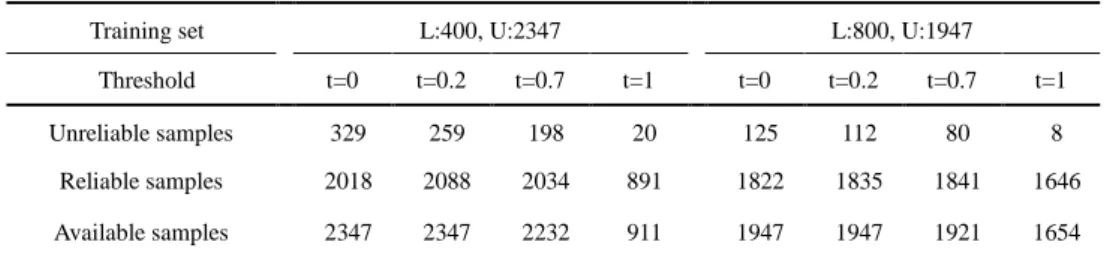
Table 4: The number of the reliable samples, unreliable samples and available samples in the unlabelled dataset with different thresholds.

Training set L:400, U:2347 L:800, U:1947

Threshold t=0 t=0.2 t=0.7 t=1 t=0 t=0.2 t=0.7 t=1

Unreliable samples 329 259 198 20 125 112 80 8

Reliable samples 2018 2088 2034 891 1822 1835 1841 1646

Available samples 2347 2347 2232 911 1947 1947 1921 1654

As can be seen, if the threshold is set to 0, there will be more unreliable samples. As the

threshold increases, the reliability of the unlabelled samples is improved. Compared with the case

of

t



0

t



0.2

reliable samples is increased. Hence, the thresholding processing can effectively improve the

reliability of the unlabelled samples. However, if the threshold continues to increase, the number

of the available samples is gradually reduced. The reason is that, if the maximum probability of a

21

Figure 1, we utilize the unlabelled samples based on the class probabilities and the new LDA

method. The unlabelled samples, whose class probabilities are all set to 0, will not be utilized in

the training process. Therefore, as the threshold increases, the number of the available unlabelled

samples drops.

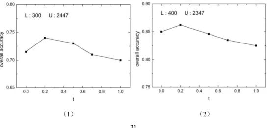
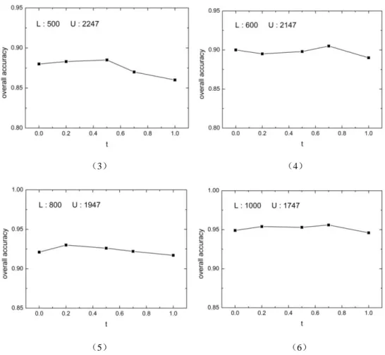
Next, we analyze the performance of our method with different thresholds. The experimental

results are shown in Figure 5. When the number of the labelled samples is less than 500, the

performance of our method is better whilst the threshold is set to be 0.2. As the number of the

labelled samples increases, the recognition accuracy is almost the same at different thresholds, in

other words, the impact of the thresholding processing becomes weak. This is because the generalization ability of the CNN model is weak when the labelled samples are insufficient.

Compared with the case of

t



0

t



0.2

increase the threshold, the number of the available unlabelled samples drops and the recognition

accuracy become worse. As the number of the labelled samples increases, the generalization ability of the CNN model is improved. As a result, the reliability of the unlabelled samples is

improved, and the impact of thresholding processing is weaker. Thus, in order to achieve the best

recognition performance, the threshold should be set to 0.2.

（3） （4）

（5） （6）

Figure 5: The recognition accuracy of our method at different thresholds and different training dataset partitions.

4.2 Comparison with other semi-supervised methods

In this section, we compare the performance of our method with that of the semi-supervised ladder network model [25], Pi model and temporal ensembling model [26]. The semi-supervised

ladder network model combines the semi-supervised learning and deep learning methods. Based

on the self-ensembling method, the Pi and temporal ensembling models are both semi-supervised

CNN methods.

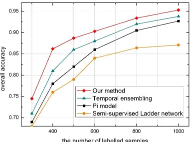
4.2.1 Recognition accuracy

First, we compare the overall accuracy of these methods. As shown in Figure 6, our method outperforms the semi-supervised ladder network. The reason is that the ladder network is

23

CNN model used in our method. Furthermore, our method is superior to the other two models.

This because the Pi and temporal ensembling models utilize the CNN to predict the labels of the

unlabelled samples. According to the predicted labels, the unlabelled component of the loss

function is obtained. However, if the initial labelled samples are insufficient, the generalization ability of the CNN is weak. Therefore, the reliability of the predicted labels is low and the

unlabelled samples are not contributing to the augmentation of the system performance. In

contrast, our method can accurately estimate the class probabilities of the unlabelled samples.

Based on the class probabilities, the impact of the unlabelled samples is well controlled in the

training process. As a result, the reliability of the unlabelled samples is improved and the recognition accuracy is increased.

Figure 6: The recognition accuracy of our method, temporal method, Pi model and semi-supervised ladder network with different partitions of the training dataset.

4.2.2 Training time

To evaluate the computation complexity of our method and the other three semi-supervised

methods, we calculate the average training time for each epoch. During the training process, the

set to 400. The experiments are implemented in the Pytorch 0.3.1 framework. And the main

configurations of the computer are: GPU: Tesla K20c; video memory: 4G; operating system:

Ubuntu 16.04.

Table 5: The running time of each epoch of our method, temporal method, Pi model and semi-supervised ladder metwork trained. All the four methods are trained by 600 labelled samples and 2147 unlabelled samples.

Methods Training time (sec/epoch )

Our method 2.53

Temporal ensembling 1.56

Pi model 2.45

semi-supervised ladder network 5.08

As shown in Table 5, the average training time of our method is 2.53sec/epoch, much less

than that of the semi-supervised ladder network. The reason is that the structure of the ladder

network is complex than that of the CNN used in our method. Thus there are more parameters that need to be trained in the ladder network, resulting in longer training time. Besides, the average

training time of the Pi model and temporal ensembling model is less than that of our method. This

is because the Pi and temporal ensembling models utilize the CNN to predict the labels of the

unlabelled samples. Afterwards, the unlabelled component of the loss function is obtained based

on the predicted labels. Thus, the computation complexity of the two methods is less than our method. However, our method can effectively maintain the reliability of the unlabelled samples.

Although the computation complexity of our method is increased, the recognition accuracy is also

improved.

5.

Conclusion

25

method has been presented in this paper. In the training process, the class probabilities are utilized

to control the impact of the unlabelled samples. As a result, the reliability of the unlabelled

samples is enhanced and the SAR-ATR accuracy of our method is improved. The contributions of

this paper are summarized as follows.

(1) We utilized the CNN to extract the features of the samples, and then the class probabilities of

unlabelled samples were obtained by the softmax function.

(2) To improve the reliability of unlabelled samples, we performed thresholding processing on the

class probabilities.

(3) Based on the class probabilities, a new LDA method was designed to utilize the unlabelled samples. As a result, the recognition accuracy was improved.

We performed the experiments on the MSTAR dataset. First, we verified the effectiveness of

the relevant steps used in our method. Then we compared the performance of our method with that

of the other semi-supervised methods. From the experimental results, we conclude that our

method can effectively improve the SAR-ATR accuracy despite the lack of the labelled samples.

Acknowledgements

This research was funded by the National Natural Science Foundation of China (No.61771027, No.61071139, No.61471019, No.61501011, and No.61171122). E. Yang is supported in part under the RSE-NNSFC Joint Project (2017-2019) (No.6161101383) with China University of Petroleum (Huadong).

H. Zhou was supported by UK EPSRC under Grant EP/N011074/1, Royal Society-Newton Advanced Fellowship under Grant NA160342, and European Union’s Horizon 2020 research and innovation program under

the Marie-Sklodowska-Curie grant agreement No 720325.

Compliance with Ethical Standards

Conflict of Interest

The authors declare that they have no conflict of interest.

Ethical Approval

This article does not contain any studies with human participants performed by any of the authors.

References

1. Moreira A, Prats-Iraola P, Younis M, Krieger G. A tutorial on synthetic aperture radar. IEEE Geosci Remote Sens Mag 2013;1(1):6-43.

2. Wang G, Tan S, Guan C, Wang N, Liu Z. Multiple model particle flter track-before-detect for range ambiguous radar. Chin J Aeronaut 2013;26:1477-87.

3. Gong M, Su L, Jia M, Chen W. Fuzzy clustering with a modified MRF energy function for change detection in synthetic aperture radar images. IEEE Trans Fuzzy Syst 2014;22:98-109.

4. Chen H, Zhang F, Tang B, Yin Q, Sun X. Slim and efficienct neural network design for resource-constrained SAR target recognition. Remote Sens 2018;10(10):1-15.

5. Zhang F, Hu C, Yin Q, Li W, Li H, Hong W. Multi-aspect-aware bidirectional LSTM networks for synthetic aperture radar target recognition. IEEE Access 2017;5:26880–91.

6. Zhang S, He B, Rui N, Wang J, Han B, Lendasse A. Fast image recognition based on independent component analysis and extreme learning machine. Cogn Comput 2014;6(3):405-22.

7. Garagnani M, Wennekers T, Pulvermüller F. Recruitment and consolidation of cell assemblies for words by way of hebbian learning and competition in a multi-layer neural network. Cogn Comput 2009;1(2):160-76. 8. Yan X. Dissociated emergent-response system and fine-processing system in human neural network and a

heuristic neural architecture for autonomous humanoid robots. Comput Intell Neurosci 2011;3(2):367-73. 9. Gao F, Ma F, Zhang Y, Wang J, Sun J, Yang E, Hussain A. Biologically inspired progressive enhancement

27

10. Spratling M. A hierarchical predictive coding model of object recognition in natural images. Cogn Comput 2017;9(2):151-67.

11. Ren P, Sun W, Luo C, Hussain A. Clustering-oriented multiple convolutional neural networks for single image super-resolution. Cogn Comput 2018;10(1):165-78.

12. Chen Y, Jiang H, Li C, Jia X, Ghamisi P. Deep feature extraction and classification of hyperspectral images based on convolutional neural networks. IEEE Trans on Geosci Remote Sensing 2016;54(10):6232-51. 13. Amrani M, Jiang F. Deep feature extraction and combination for synthetic aperture radar target classification. J

Appl Remote Sens 2017;11(4):1.

14. Zhao J, Guo W, Cui S, Zhang Z, Yu W. Convolutional neural network for SAR image classification at patch level. Geoscience and Remote Sensing Symposium IEEE 2016;945-8.

15. Chen S, Wang H. SAR target recognition based on deep learning. International Conference on Data Science and Advanced Analytics IEEE 2015;541-7.

16. Gao F, Huang T, Sun J, Wang J, Hussain A, Yang E. A new algorithm of SAR image target recognition based on improved deep convolutional neural network. Cogn Comput 2018;1-16.

17. Liu B, Yu X, Zhang P, Tan X, Yu A, Xue Z. A semi-supervised convolutional neural network for hyperspectral image classification. Remote Sens Lett 2017;8(9):839-48.

18. Fu Z, Zhang F, Yin Q, Li R, Hu W, Li W. Small sample learning optimization for resnet based sar target recognition. International Geoscience and Remote Sensing Symposium IEEE 2018;2330-3.

19. Zhu X, Rogers T, Qian R, Kalish C. Humans perform semi-supervised classification too. National Conference on Artificial Intelligence AAAI Press 2007;864-9.

20. Haeusser P, Mordvintsev A, Cremers D. Learning by association — a versatile semi-supervised training method for neural networks. In Proceedings of IEEE conference on computer vision and pattern recognition 2017;626-35.

21. Gibson B, Rogers T, Zhu X. Human semi-supervised learning. Top Cogn Sci 2013;5(1):132-72.

22. Hänsch R, Hellwich O. Semi-supervised learning for classification of polarimetric SAR-data. Geoscience and Remote Sensing Symposium IEEE 2010;987-90.

23. Uhlmann S, Kiranyaz S, Gabbouj M. Semi-supervised learning for ill-posed polarimetric SAR classification. Remote Sens 2014;6(6):4801-30.

24. Basu S. Semi-supervised learning. Pacific-Asia Conference on Advances in Knowledge Discovery and Data Mining 2010;588-95.

25. Leng Y, Xu X, Qi G. Combining active learning and semi-supervised learning to construct SVM classifier. Knowledge-Based Syst 2013;44:121-31.

26. Zhang X, Song Q, Liu R,Wang W, Jiao L. Modified co-training with spectral and spatial views for semisupervised hyperspectral image classification. IEEE J. Sel. Top. Appl. Earth Observ. Remote Sens 2014; 7(6):2044-55.

27. Lv L, Zhao D, Deng Q. A semi-supervised predictive sparse decomposition based on task-driven dictionary learning. Cogn Comput 2016;9(1):1-10.

28. Ding S, Xi X, Liu Z, Qiao H, Zhang B. A novel manifold regularized online semi-supervised learning model. Cogn Comput 2018;10(1):49-61.

29. Rasmus A, Valpola H, Honkala M, Berglund M, Raiko T. Semi-supervised learning with ladder networks. Compu Sci 2015;9 Suppl 1(1):1-9.

29

30. Laine S, Aila T. Temporal ensembling for semi-supervised learning. International Conference on Learning Representations 2017.

31. Le T, Kim S. A hybrid selection method of helpful unlabeled data applicable for semi-supervised learning algorithms. The IEEE International Symposium on Consumer Electronics 2014;1-2.

32. Li Y, Zhou Z. Towards making unlabeled data never hurt. IEEE Trans Pattern Anal Mach Intell 2015; 37(1):175–88.

33. Szegedy C, Liu W, Jia Y, Sermanet P, Reed S, Anguelov D. Going deeper with convolutions. IEEE Conference on Computer Vision and Pattern Recognition 2015;1-9.

34. Lawrence S, Giles C, Tsoi C, Back A. Face recognition: a convolutional neural-network approach. IEEE Trans on Neural Netw 1997;8(1):98-113.

35. Moskowitz L. The LDA - an integrated diagnostics tool. IEEE Aerosp Electron Syst Mag 1986;1(7):22-6. 36. Huan R, Liang R, Pan Y. SAR target recognition with the fusion of LDA and ICA. International Conference on