System G Data Store: Big, Rich Graph Data Analytics in the Cloud

(1)

System G Data Store: Big, Rich Graph Data Analytics in the Cloud

Mustafa Canim and Yuan-Chi Chang

IBM Thomas J. Watson Research Center P. O. Box 218, Yorktown Heights, New York, U.S.A.

{mustafa, yuanchi}@us.ibm.com

Abstract—Big, rich graph data is increasingly captured through the interactions among people (email, messaging, social media), objects (location/map, server/network, product/catalog) and their relations. Graph data analytics, however, poses several intrinsic challenges that are ill fitted to the popular MapReduce programming model. This paper presents System G, a graph data management system that supports rich graph data, accepts online updates, complies with Hadoop, and runs efficiently by minimizing redundant data shuffling. These desirable capabilities are built on top of Apache HBase for scalability, updatability and compatibility. This paper introduces several exemplary target graph queries and global feature algorithms implemented using the newly available HBase Coprocessors. These graph algorithmic coprocessors execute on the server side directly on graph data stored locally and only communicates with remote servers for the dynamic algorithmic state, which is typically a small fraction of the raw data. Performance evaluation on real-world rich graph datasets demonstrated significant improvement over traditional Hadoop implementation, as prior works observed in their no-graph-shuffling solutions. Our work stands out at achieving the same or better performance without introducing incompatibility or scalability limitations.

Keywords-graph data management, graph analytics, HBase, Coprocessor

I. INTRODUCTION

An ACM Computing Surveys article in 1984 began its introduction in the following words:Graph theory is widely applied to problems in science and engineering. Practical graph problems often require large amounts of computer time[1]. In today’s graph applications, not only did the graph size grow, the data characterizing vertex and edges becomes richer and more dynamic, which enables new hybrid content and graph analysis.

This paper proposes a big graph data management system named System G as an add-on to, as opposed to replac-ing, the popular big data processing framework Apache Hadoop [2]. Years of effort from the open source community and the industry invested in analytical libraries can be leveraged if System G remains compatible and its data serves multiple purposes of graph processing, text mining and machine learning. For System G on Hadoop to be practical, however, it must address two challenges. First, it must accept incremental updates to the data, including deletes and inserts that change graph topology as well as the associated metadata and rich content. This is because a read-only

system significantly restricts its usefulness to many practical applications. Second, it must alleviate redundant graph data shuffling in the MapReduce programming framework, as identified in [3][4][5]. The overhead in network and storage I/O appears in iterative graph algorithms like connected components as well as targeted queries such as nearest neighbors.

Our proposed System G overcomes the above challenges by building on top of Apache HBase and its new Copro-cessor feature [6]. Our system stores graph data, including metadata and unstructured content, in the tables managed by HBase. We leverage the fact that HBase is closely integrated with Hadoop Distributed File System (HDFS) and thus achieves compatibility with ”legacy” Hadoop jobs by simply sourcing data locally from HBase to Hadoop data nodes. The system further leverages HBase record transaction support to insert, update and delete graph data. Incremental changes remain transparent to Hadoop jobs, which can read records in HBase by fixed versions or timestamps.

The main contribution presented in this paper focuses on how our graph algorithms can minimize data shuffling by applying server side processing, i.e. HBase Coprocessors, extensively. As pointed out in [3], the MapReduce frame-work does not directly support iterations and there is no program state retained between successive iterations. In the context of graph data processing, this means the entire graph data repeatedly gets partitioned, joined, merged and sorted across distributed computing nodes, incurring unnecessary network and disk I/O. Besides our proposed system, we are unaware of other graph processing framework to simulta-neously address Hadoop compatibility, update functionality and query efficiency. Additional benefit comes from our algorithms implemented through pluggable HBase Copro-cessors, their forward compatibility continues to benefit from future releases of Hadoop and HBase.

The rest of the paper is structured as follows. Section II gives an overview of the proposed graph data management system, including a brief introduction to Apache HBase and its new Coprocessor feature. Section III describes the K-neighborhood and the K-(s,t) shortest path algorithms as examples of target graph queries implemented on server side processing. Section IV illustrates PageRank and connected components as examples of global queries on server side processing. Section V presents performance benchmarking

(2)

Region Server HRegion HRegion HFile HFile Region Server HRegion HRegion HFile HFile Region Server HRegion HRegion HFile HFile HBase Client

Hadoop Distributed File System

Master Server(s)

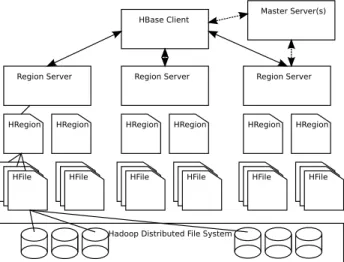
Figure 1. HBase cluster consists of one or multiple master servers and many region servers, each of which manages data rows partitioned into HRegions. HRegion persists data in HFile stored in HDFS.

results on three social network data sets. In Section VI we discuss related work. Finally, we conclude the paper with the lessons learned and future directions.

II. SYSTEMOVERVIEW

We model interactions between pairs ofobjects, including structured metadata and rich, unstructured textual content, in the graph representation materialized as adjacency list known as edge table. An edge table is stored and managed as an ordered collection of row records in an HTable by Apache HBase [6]. Since Apache HBase is fairly new to the research community compared to Hadoop, we first describe its architectural foundation briefly to lay the context of its latest feature known as Coprocessor, which our algorithms make use of for graph query processing.

A. HBase Basics

Apache HBase is a non-relational, distributed data man-agement system modeled after Google’s BigTable [7]. Writ-ten in Java, HBase is developed as a part of the Apache Hadoop project and runs on top of Hadoop Distributed File System (HDFS). Unlike conventional Hadoop whose saved data becomes read-only, HBase supports random, fast insert, update and delete (IUD) access at the granularity of row records, mimicking transactional databases. Prominent HBase partitioners include Facebook [8] and many oth-ers [9].

Fig. 1 depicts a simplified architectural diagram of HBase with several key components relevant to this paper. An HBase cluster consists of master servers, which maintain HBase metadata, and region servers, which perform data operations. When an HBase client calls to create an HTable, a master server assigns one or more of the table’s HRegions to the region servers. A client directly communicates with region servers via remote procedure call.

HBase region server, similar to data node in Hadoop, manages HRegions assigned to it. IUD operations of row records as well as HRegion splitting and compaction are executed by the region servers. An HRegion may be further divided into one or multiple HFiles stored in HDFS for availability. One can create arbitrary number of columns since a column and its value is stored as a column name-value pair.

Row records in HBase may be viewed as a sorted key-value map, which starts with a row key, followed by column families and their column values. Row key is equivalent to the notion of primary key in RDBMS tables. Unlike parallel databases, HBase organizes rows with their keys sorted in alphanumeric order. Rows in sorted order are then partitioned into HRegions, which keep track of start (the lowest) and end (the highest) keys within the region. HBase client connects directly to the region holding a record by checking the region map. Our algorithms extensively take advantage of range partitioning to minimize the amount of data shuffling.

Unlike RDBMS, there is no in-place update in HBase to overwrite an existing row. Instead, HBase appends updated row records, due to either updated values or brand new columns, at the end with a version number and timestamp. HBase merges the appended data to respond to row requests. One benefit of the ’write append’ is versioning. Our PageR-ank implementation took advantage of HBase versioning to compute differences of the PageRank vector between current and previous iterations.

B. HBase Coprocessors

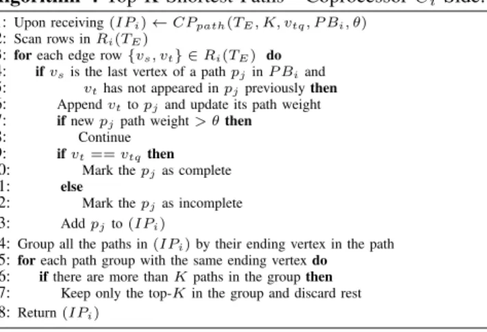
HBase’s Coprocessor feature was first introduced in ver-sion 0.92, released in January 2012 [10]. Like HBase itself, the idea of Coprocessors was inspired by Google’s BigTable coprocessors. It was recognized that pushing the computa-tion to the server where user deployed code can operate on the data directly without communication overheads can give further performance benefit. Endpoint CP, one of the two programming hooks, can be invoked by an HBase client to execute at the target region. Results from the remote executions can be returned directly to the client, in the example of counting rows, or inserted into other HTables in HBase, as exemplified in our algorithms.

Fig. 2 depicts the runtime scenario of an Endpoint CP processing data in an HRegion locally in the region server host. A CP may scan every row from the start to the end keys in the HRegion or it may impose filters to retrieve a subset in selected rows and/or selected columns. Note the row keys are sorted alphanumerically in ascending order in the HRegion and the scan results preserve the order of sorted keys. In addition to reading local data, a CP may be implemented to behave like an HBase client. Through the Scan, Get and Put methods and their bulk processing variants. a CP can access other HTables hosted in the HBase cluster. For example,

(3)

Region Server HRegion A10B13, .... A10B25, .... A10B34, .... A10B61, .... A21B41, .... A41B51, .... B14C21, .... B14D12, .... B14F13, .... B61A10, .... B61A21, .... C41C42, .... G12B12, .... G12C31, .... G12C41, .... H41H20, .... H42K41, .... L12K40, .... L23B41, .... Scan Filter Scan Coprocessor Scan Get Get Put Put Put Put Process local data

Read data from other tables in bulk or lookups Write data to other tables in bulk inserts or updates

Figure 2. Endpoint Coprocessors read data from local HRegion and can optionally read from and write to other HTables in bulk or lookups.

a CP can request to scan another table, at the expense of remote procedure calls (RPC). Similarly a CP can insert rows into another table through RPC. The latter scenario usually applies when the results of CP processing are too large to be returned to the client.

The flexibility of CP introduced many possibilities to process local data in a targeted way. On the other hand, spreading the reads and writes across the cluster and incur-ring RPC penalty must be carefully worked into algorithm design as presented in the following sections.

C. Graph Processing on HBase

We define a rich graph representation G =

{V, E, M[V, E], C[V, E]}, where V is the set of vertex, E

is the set of directional edges, M[V, E] is the structured metadata associated with a vertex or an edge, andC[V, E]

is the unstructured context respectively. To map the graph representation to an HTable, we first format the vertex identifier v ∈ V into a fixed length string pad(v). Extra bytes are padded to make up for identifiers whose length is shorter than the fixed length format. The padding aims to preserve the natural representation of the id’s for other applications and avoids id remapping.

The row key of a vertex v is its padded id pad(v). The row key of an edge e = {vs, vt} ∈ E is encoded as the concatenation of the fixed length formatted strings of the source vertex pad(vs), and the target vertex pad(vt). The encoded row key thus will also be a fixed length string

pad(vs) +pad(vt). This encoding convention guarantees a vertex’s row always immediately proceeds the rows of its outbound edges in an HTable. Our graph algorithms exploit the strict ordering to join ranges of two tables. Respective metadata M[V, E] and content C[V, E] are stored in the

column families, which expand as needed. Fig. 2 included a simple example of encoded graph table, whose partitioned HRegion is shown on the left. In this table, a vertex is encoded as a string of three characters such as ’A10’, ’B13’, ’B25’, ’A21’, etc. A row key encoded like ’A10B13’ represents a graph edge from vertex ’A10’ to ’B13’. The current layout retains minimal clustering, only a vertex and its immediate outbound edges are stored consecutively, although System G can adopt partitioning techniques such as [11].

We conclude this section with a list of HBase properties our algorithms exploit in order to achieve scalability while maintaining compatibility and updatability, namely,

• Server side processing, i.e. HBase Coprocessors, that can access multiple tables in bulk and lookups • Range partitioning based on row keys that enables more

sequential reads of rows in a key range as opposed to more expensive random reads

• Schema-less, expandable rows to add new columns as needed

• Versioning of rows to inspect change between versions • Rich metadata and content managed within the graph layout for joint graph structural and content analysis III. PARALLELPROCESSING OFTARGETQUERIES

HBase is particularly suited for target graph queries, i.e. computation that only involves small portions of the graph data but not the entire graph. For brevity, this section illus-trates algorithms for two target queries using CP. Interested readers can infer other target query processing using CP. Table I summarizes the notations.

Table I NOTATIONS

TA(CF1:CX, CF2:CY) Table A created on HBase

with column familyCF1, columnCX and column familyCF2, columnCY

Ci ithCP running on Regioni

CPf(TA) CP function running on tableTA

(X, TB)←CPf(TA, S) CP functionftakes parameterS and returns valueXto client outputs bulk results into tableTB

{u, v_} Graph edge from vertexuto vertexv Ri(TA) Region ofTAprocessed byCi

A. K-Neighborhood

By K-Neighborhood, we mean finding the neighboring vertices that are within K hops from the queried vertex

vq. K-Neighborhood may be processed by purely graph topology alone or context/content dependent based on the metadata carried by the edges. As defined in Section II-C, the row key of an edge e = {vs, vt} ∈ E is encoded as the concatenation of the fixed length formatted strings of the source vertex pad(vs), and the target vertex pad(vt). Because of this encoding, an HBase client can efficiently find edges that originates from vertexvq. It is thus trivial to find all the vertices one hop away fromvq.

(4)

One can simply repeat the one-hop lookup stepK times or take advantage of CP for more server side processing. Details of the CP implementation are given in Algorithm 1 (Client side) and Algorithm 2 (Server side). Given a query vertexVq, the query client first initializes a vertex setV S= {Vq}. The client then invokes CP function(V Si)←CPscan

(TE, V S) on the graph edge table TE. The client-side

invocations target specifically to the regions holding theV S. After receiving the client invocation, each invoked CP scans its own region Ri(TE). For each edge {vs, vt},Ci checks if the source vertexvsis in the vertex setV S. Newly found target vertices that can be reached by vertices in V S are put into the result set V Si. CPs then return their setsV Si to the client. Client merges the vertex sets received from CPs to updateV Swith new found neighbors. The iterations continue until all neighbors withinK hops are identified.

In this fairly simple application of CP in server side processing, processing efficiency mainly comes from: first, CPs, knowing vertices already found in V S, only return the new vertices; second, CP can take additional input parameters to match metadata and content of the edges and process the matching or scoring on the server side. For example, find friends of friends interested in classical music. Algorithm 1 K-Neighborhood - Client Side:

1: Given vertexVq

2: AddVqinto vertex setV S

3: fori= 1 toKdo

4: CP request to regions holdingvsinV S:(V Si)←CPscan(TE, V S)

5: whereV Siis the vertex set returned to client fromCPi

6: Wait CPs to complete

7: Merge vertex sets returned from CPs

8: V S=∪iV Si

9: ReturnV S

Algorithm 2 K-Neighborhood - CoprocessorCi Side:

1: Upon receiving(V Si)←CPscan(TE, V S)

2: Scan rows inRi(TE)

3: foreach edge row{vs, vt} ∈Ri(TE) do

4: if vsis inV Sandvtis not inV Sthen

5: AddvtintoV Si

6: ReturnV Si

B. K-(s,t) Shortest Paths

Following the introduction of CP used in K-Neighborhood query, we now describe a more sophisticated use case of CP, using K-(s,t) simple shortest path as an example. The top-K simple shortest path problem is defined as finding the K shortest, loopless paths, each of which traverses across a sequence of vertices connected by edges from the source vertex to the target vertex. By loopless, we mean a vertex does not appear more than one time in a valid path. By shortest, we mean the number of hops or aggregated measure of edge weights is the smallest numerically. For a connected graph, by definition the single shortest path between any pair of vertices can always be found. However, note the K-th loopless shortest paK-ths may not exist. While in-memory

algorithms exist for this problem [12], what is described here is the only solution we are aware of aimed at distributed, server side processing. For cleanliness of the description, we present the algorithm without including context or content matching, knowing in practice a K-(s,t) shortest path query is often casted in context. For example, what are the ways that a breaking news reaches an individual?

Algorithm 3Top-K Shortest Paths - Client Side:

1:Given an (s,t) pair(vsq, vtq)andK

2:Initialize an empty path bucketP Bifor each RegioniinTE

3:Addvsqto its region path bucketP Bqas the first path

4:Initialize an empty top-K path listT OP Kand set the maximal thresholdθto infinity

5:whileanyP Bihas incomplete paths pendingdo

6: foreach Regionido

7: ifCP for the region is not busythen

8: CP request to extend the incomplete paths

9: (IPi)←CPpath(TE, K, vtq, P Bi, θ)

10: foreach Regionido

11: ifCP for the region completed and returned(IPi)then

12: UpdateT OP Kandθ

13: for paths in(IPi)that reachedvtq

14: Add the remaining incomplete paths to respectiveP Bi

15: Remove incomplete paths inP Bi

16: whose path weight is greater thanθ

17:ReturnT OP K

The essence of our new algorithm may be summarized as follows. Incomplete paths originated from the queried source vertexvsqare managed at the client, which dispatches batches of these incomplete paths to respective CPs to work on their HRegions locally. The client maintains globally a top-K list of completed paths connecting the queried (s,t) pairvsqandvtq, with the maximal path threshold at the K-th shortest path. CPs append additional hops to the incomplete paths, update their path weights and only return those, either complete or incomplete paths, that beat the current path threshold. Incomplete paths returned by the CPs to the client are added to the batches waiting to be evaluated. The search process continues until there are no more incomplete paths for CPs to evaluate.

One might view our algorithm as breadth first search (BSP)asynchronously executed across CPs with batches of incomplete paths and the current path threshold exchanged only to the HRegions holding the next hop. Depending on the temporary load of respective servers, a CP may complete its processing faster or slower than the other CPs. The client-side controller, however, does not wait to hear from all the CPs but continues to dispatch work to CPs that have finished their previous batch. Such asynchronous processing, by design is to accelerate the finding of the first K completed paths, even if they are not the final results. Finding the first K shortest paths establishes the maximal path threshold, which is used by subsequent CP processing to prune out non-result paths.

Details of the CP implementation are given in Algorithm 3 (Client side) and Algorithm 4 (Server side). Given (s,t) pair (vsq, vtq) and K, the query client dispatches

(5)

non-Algorithm 4 Top-K Shortest Paths - CoprocessorCi Side:

1: Upon receiving(IPi)←CPpath(TE, K, vtq, P Bi, θ)

3: foreach edge row{vs, vt} ∈Ri(TE) do

4: ifvsis the last vertex of a pathpjinP Biand

5: vthas not appeared inpjpreviouslythen

6: Appendvttopjand update its path weight

7: ifnewpjpath weight> θthen

8: Continue

9: ifvt==vtqthen

10: Mark thepjas complete

11: else

12: Mark thepjas incomplete

13: Addpjto(IPi)

14: Group all the paths in(IPi)by their ending vertex in the path

15: foreach path group with the same ending vertexdo

16: ifthere are more thanKpaths in the groupthen

17: Keep only the top-Kin the group and discard rest

18: Return(IPi)

empty path buckets P Bi to respective table regions. A CP is invoked with four parameters: K, the target vertex

vtq, a batch of incomplete paths P Bi and the maximal thresholdθ for an eligible path in the top-K. There are two ‘for’ loops at the client side described in Algorithm 3 to illustrate the asynchronous processing aspect. The first ‘for’ loop dispatches new work when a CP becomes available to receive the next batch. The second ‘for’ loop adds results

(IPi)returned by CPCito the path buckets and updates the top-K path list T OP K for paths reachingvtq. In practice, we implemented the two ‘for’ loops as threads to dispatch work and receive results from CP calls.

On the server side, the CP scans its region to append vertices to the path bucket received P Bi. It prunes out paths whose weights exceeded the current threshold θ. It further optimizes by pruning extra paths ending at the same vertex when there are more than K of them. Due to the required ”loopless” property, a CP must check the path before appending a new vertex that it has not appeared in the path downstream fromvsq. This is unlike single shortest path where only the path weight needs to be retained, since any loop is automatically eliminated.

It is worthy pointing out that our algorithm does not conform to the Bulk Synchronous Parallel model nor does its asynchronous processing impact the correctness of the results. This and the connected component algorithm de-scribed in Section IV-B are likely to converge much faster at runtime by removing the synchronization barrier.

IV. PARALLELPROCESSING OFGLOBALQUERIES

Global graph queries identify properties or compute fea-tures for the entire graph. In many cases, algorithms taking advantage of CP exceed the performance of vanilla MapRe-duce implementation. Due to page limits, we illustrated two algorithms to inspire further work.

A. PageRank

PageRank is well known and we follow the definition in [5]. Our algorithm implementation applied four CPs to

Client Coprocessor Ci Populate TPR Scan TE Populate TPR Create TPR Populate TPR Summary Drop & Recreate TPR Summary Aggregate TPR Summary Scan TE and TPR Populate TPR Summary Scan TPR Summary Update TPR

Get Absolute Diff on TPR Summary

Scan TPR Return diff Repeat Iterations Terminate if difference is low

Figure 3. Client-Coprocessor call graph to compute PageRank

avoid as much graph data shuffling as possible. The first CP initializes an HBase table where the PageRank values of vertices are held. The second CP scans the edges and outputs partial results into a temporary HBase table. The third CP aggregates these partial results and updates the PageRank table. The fourth CP compares changes in the PageRank values of vertices to decide as to whether stop or continue the iteration. The call graph to invoke the CPs at different phases of the algorithm is illustrated in Figure 3 and the details of the client side and server side implementations are given in Algorithm 5 and Algorithm 6 respectively.

Initialization:

The client first creates an HBase table called TP R(CF :

CoutEdges, CF : CpageRank). This table keeps the PageR-ank of each vertex in the graph and is updated in each iteration as new PageRank values are computed. TP R has one row for every vertex in the graph. The table has two columns:CoutEdges keeps the fanout andCpageRank keeps the initial value equal to 1/|V| . The client calls a CP function(TP R)←CPpopulateP Rtable(TE,|V|)on the graph edges table TE. Upon receiving this function call, each CP

Ci scans its own region of the tableRi(TE)and inserts the discovered vertex IDs into TP R. For each vertex a new row is created where the key of the row is the vertex ID. Since the edges are sorted based on source IDs of edges, the fanout counts are easily computed and inserted intoTP R.

Iterations:

WithTP Rpopulated by CPs, the client then starts PageR-ank iterations. At the end of each iteration updated PR values are written back to this table. An iteration con-sists of three phases. In the first phase a summary table

TP RSummary(CF : CRi) is populated and in the second

phase this summary table is used to update PageRank values of the vertices inTP R. In the third phase the CPs calculate the delta in the PageRank vector to meet convergence crite-rion.TP RSummary is a temporary table and is recreated for every iteration. It stores partial PageRank results submitted

(6)

Algorithm 5 PageRank on HBase - Client Side:

1: CreateTP R(CF:CoutEdges, CF:CpageRank)

2: (TP Rwill have the final output)

3: CP requestR1:(TP R)←CPpopulateP Rtable(TE,|V|)

4: where|V|is the number of vertices in the graph

6: DropTP RSummaryif exists

7: CreateTP RSummary(CF:CRi)

8: CP requestR2:

9: (TP RSummary)←CPpopulateSummaryT able(TE)

11: CP req.R3:(TP R)←CPprAggregate(TP RSummary)

13: CP requestR4:(δi)←CPgetP RAbsoluteDif f(TP R)

14: whereδiis the total error rate forRi(TP R)

15: Compute total error rateγ=∑n_i₌₁δi

16: if γ¡ total acceptable error rate then

17: Terminate

18: else

19: Go to Line 6 to continue iterations

from each region. The partial results are then aggregated and weighted for PageRank update.

The client first calls a CP function called

(TP RSummary) ← CPpopulateSummaryT able(TE) on the graph edges table TE. After receiving this function call each coprocessor Ci scans its own region of the table

Ri(TE). For each source ID of the edges the PageRank value tableTP Ris probed to get the vertex’s latest PageRank value and fanout. The PageRank value is divided by fanout and the edge weight is calculated. For each destination ID this edge weight is inserted into TP RSummary table as a new column. CPpopulateSummaryT able can also subtotal all the edge weights destined to the same vertex ID.

The CP function(TP R)←CPprAggregate

(TP RSummary) is launched next to all the regions of

TP RSummary. After receiving this function call each co-processorCi scans its own region of the tableRi(TE). For every row, its column values are added to compute the next update to the PageRank value, which is then inserted back intoTP R.

Finally the client gets help from CPs to compute the delta between the current and previous PageRank vectors.(δi)←

CPgetP RAbsoluteDif f(TP R)is called on the PageRank table

TP R. The CPs then scan their regions in parallel, read the latest two versions of the rows ut1 and ut2 and compute their differences. Iterations continue if the delta exceeded the convergence criterion.

Between our PageRank algorithm designed around CP and the popular MapReduce implementation, the most notable difference is that the graph data table TE stays local and does not get reshuffled across network. In an MapReduce implementation, TE must be emitted by the mappers such that the graph topology can be joined with the PageRank vector in the reducer phase. Mapper emitted records will be shipped to another server where their reducer propagates value along the edges. The record shipping incurs unnec-essary network and disk I/O. In contrast, in our algorithm, CPs can work on the table regions locally by bringing the

Algorithm 6PageRank on HBase - CoprocessorCi Side:

1:if R1==(TP R)←CPpopulateP Rtable(TE,|V|) then

3: foreach edge row{u, v} ∈Ri(TE) do

4: Count outgoing edges ofu

5: PUT new rowru

6: ru= (numOf OutEdges(u),1/|V|)intoTP R

7: where row key isu

8: PUT new rowrv

9: rv= (null,1/|V|)intoTP R

10: where row key isv

11: Return

12:if R2==

13: (TP RSummary)←CPpopulateSummaryT able(TE) then

16: GETP R(u)fromTP R

17: GETnumOf OutEdges(u)fromTP R

18: PUT new row r intoTP RSummary

19: wherer= (P R(u)/numOf OutEdges(u))

20: and row key isv

21: Return

22:if R3==(TP R)←CPprAggregate(TP RSummary) then

23: Scan rows inRi(TP RSummary)

24: foreach edge rowr∈Ri(TP RSummary) do

25: ReadedgeP Rvaluefrom each column and add up

26: Compute PageRank ofvwherevis the key ofr

27: P R(v) = (1−d)/|V|+d∗edgeP Rvalue

28: PUT new rowr= (P R(v))intoTP R

29: where row key isv

30: Return

31:if R4==(δi)←CPgetP RAbsoluteDif f(TP R) then

32: Setδito 0

33: Scan latest two versions of rows inRi(TP R)

34: for each row versionut1,ut2∈Ri(TP R) do

35: Add difference|ut1−ut2|intoδi

36: Returnδi

much smaller PageRank vector to the region. It is thus not surprising our approach is more suited to query big, rich graphs.

B. Connected Components

Connected components (CC) is also a well known graph problem that identifies groups of vertices linked by edges. Our CC algorithm not only takes advantage of no shuffling but also leverages HBase random access to gain significant speedup. Our algorithm is founded in the idea of label propagation, where each vertex has its own label in the be-ginning and the labels are merged as two labelled ’bubbles’ meet on the graph edges. In total, we applied three CPs for parallel processing and one client-side connected component merging routine. The first CP initializes an HBase table where labels of vertices are held. The second CP scans local graph data and outputs partial results into a temporary HBase table. The third CP counts the number of rows in the temporary table to decide if the iteration should terminate. If not, the client reads the temporary table, merges its partial results and updates the label table. The call graph to invoke CPs at different phases of the algorithm is illustrated in Figure 4 with details of the client side and server side implementations given in Algorithm 7 and Algorithm 8 respectively.

(7)

Initialization:

The client first creates an HBase table calledTLabel(CF :

ClabelString, CF : ClabelSize). This table keeps the label of each vertex in the graph and is updated throughout the iterations as new labels assigned to the vertices. The table has one row for every vertex and thus has a size |V|. Its two columns keep a label and an estimated number of vertices having that same label. We refer to the group of connected vertices with the same label as a ’bubble’ as visually depicted in Figure 5. The more vertices a bubble contains, the bigger it is.TLabel is created by client calling a CP(TLabel)←CPpopulateLabelT able(TE, ω)on the graph edges table TE whereω is the minimum bubble size. The CP scans its own region ofTE and counts a vertex’s fanout. If the fanout is greater thanω, the vertex ID is inserted into

TLabel. When two bubbles merge, vertices in the smaller bubble take the label of the bigger bubble to minimize updates. Client Coprocessor Ci Populate TLabel Scan TE Populate TLabel Create TLabel Populate TBubble Drop & Recreate TBubble

Count rows on TBubble

Scan TE and TLabel Populate TBubble Scan TBubble Count rows Repeat Iterations Number of rows Terminate if TBubble is empty Scan TBubble Merge buckets Update TLabel

Figure 4. Client-Coprocessor call graph to identify connected components

Iterations:

With TLabel populated by CPs, the client then kicks off iterations to identify connected subgraphs. At the end of each iteration updated labels are written back to this table. An iteration consists of three phases. First, a bubble table

TBubbleis created on the connections among bubbles. Next, a simple row count of the tableTBubbletells how many more bubbles to merge. Last, a client side algorithm readsTBubble progressively to merge bubbles and update the vertices with new labels inTLabel.TBubbleis recreated for every iteration. The client first calls a CP function called (TBubble) ←

CPupdateBubbleT able(TE)on the graph edges tableTE. After receiving this function call each CP scans its own region of

Ri(TE). For every edge,TLabel is probed to get the label of vertex IDs. If the vertices have different labels a new row is inserted into TBubble to record their labeled bubbles are in fact connected and thus should be merged.

The second phase starts after CPupdateBubbleT able is

done. The client calls a CP function called (λ) ←

A

B C

E

Figure 5. Our algorithm merges bubbles beyond their immediate neighbors in one step

CPgetRowCount(TBubble)on the tableTBubblewhereλis the number of rows inRi(TBubble). Each CP reports the number of rows in its region to the client, which aggregates the subtotals to estimate how many bubbles wait to be merged. The client uses the row count information to decide if all the rows inTBubblecan be read and merged in memory or it may elect to first merge those bubbles which are most connected. We skip the detailed description of this in-memory bubble merging process but wish to point out that random access in HBase enables our algorithm to merge bubbles beyond their immediate neighbors.

Algorithm 7CC on HBase - Client Side:

1:CreateTLabel(CF:ClabelString, CF :ClabelSize)

2: (TLabelwill have the final output)

3:CP requestR1:(TLabel)←CPpopulateLabelT able(TE, ω)

4: whereωis the minimum bubble size

5:Wait CPs to complete

6:DropTBubbleif exists

7:CreateTBubble(CF:CRi)

8:CP requestR2:(TBubble)←CPupdateBubbleT able(TE)

9:Wait CPs to complete

10:CP requestR3:(λ)←CPgetRowCount(TBubble)

11: whereλis the number of rows inRi(TE)

12:if λ== 0 then 13: Terminate 14:Wait CPs to complete 15:ScanTBubble 16:Merge buckets 17:UpdateTLabel

Figure 5 illustrates an example where five bubbles are interconnected by edges (A,C), (B,C), (C,D) and (B,E). Distributed connected component algorithms and their im-plementation through MapReduce takes two iterations to first merge (A, B, C, D) and then propagates to E through B. Our algorithm takes advantage of random access and can merge all five bubbles in a single iteration by reading the connectivity rows in TBubble into memory. The speedup is most significant when a graph has a large diameter, i.e. it takes many iterations to propagate bubble labels but our algorithm can accomplish in fewer iterations.

After client-side merging, the labels for vertices are up-dated inTLabel. Our algorithm performs further optimization to keep labels of the larger bubbles as they were and assign those to the smaller bubbles to minimize updates.

(8)

Algorithm 8 CC on HBase - CoprocessorCi Side:

1: if R1==(TLabel)←CPpopulateLabelT able(TE, ω)then

4: α= Count outgoing edges ofu

5: if α≥ω then

6: PUT new rowru

7: ru= (u, α)intoTLabel

8: where row key isu

9: Return

10: if R2==(TBubble)←CPupdateBubbleT able(TE) then

12: foreach edge row_{u, v_{} ∈}Ri(TE) do

13: GETLabel(u)andLabel(v)fromTLabel

14: ifLabel(u)!=Label(v)then

15: PUT new row r intoTBubble

16: wherer=Label(u)and row key isv

17: Return

18: if R3==(λ)←CPgetRowCount(TBubble) then

19: Scan rows inRi(TBubble)

20: λ= Count rows inRi(TBubble)

21: Returnλ

V. EVALUATION

We report performance evaluation results comparing global graph queries implemented via HBase coprocessors versus Hadoop MapReduce implementation. We do not compare target queries since there is no equivalent M-R job that can have a fair advantage against our algorithms, which are able to selectively access a small percentage of the data. In addition, functionality such as continuous updates while queries are being evaluated concurrently is beyond the scope of this paper, since there is also no equivalence in the base M-R framework.

We conducted experiments on one master server and twelve slave servers, each of which is a virtual machine (VM) in a computing cloud. Each VM has 4 CPU cores, 6 GB main memory and 72GB storage, all dedicatedly provisioned. On the networking side, the VMs use shared virtual and physical switches, which do make our workloads susceptible to other hosted workloads. We use vanilla HBase environment running Hadoop 1.0.1 and HBase 0.92.1 with data nodes and region servers co-located on the slave servers. There was no other significant software activity to contend with system resources.

The datasets we used in the experiments were made available by Milove et al. [13] and the Stanford Network Analysis Project [14]. We appreciate their generous offer to make the data openly available for research. For details, please see the references and we only briefly recap the key characteristics of the data in Table II. To emulate real-world content rich graph edges, the datasets were prepared with a random text string of 1 KB length attached to each edge. Some of our experiments also included keyword matching to the content column in the query processing. Table II thus listed the size of the enriched edge files on HDFS and in the HBase table. Note since column names are stored along with their values in an HTable, the on-disk size of an HTable

is usually bigger. Given a total of 72 GB main memory and 600 GB HDFS space on the entire cluster, these datasets’ sizes are commensurable to the cluster’s capacity without constantly running the Hadoop rebalancer.

Table II

KEY CHARACTERISTICS OF DATASETS IN THE EXPERIMENTS

Name Vertex Edge HDFS size HTable size Ref

YouTube 1.1 M 4.9 M 5.1 GB 5.7 GB [13]

Flickr 1.8 M 22 M 25.7 GB 28.3 GB [13]

LiveJournal 5.2 M 72 M 69.4 GB 77.5 GB [14]

A. Experiments With Target Queries

K-Neighborhood: To show the benefits of server side processing as opposed to client only processing we imple-mented both client based and CP based version of the K-Neighborhood algorithm and conducted experiments. Client based implementation scans the edges table and constructs the set of neighbors of a given vertex for each hop. A naive implementation of this approach would bring all rows from the region servers to the client side and do filtering in the client side. Instead, we used predicate filtering feature of HBase to prefilter unnecessary rows on region servers and then transfer qualifying rows to the client side. Even with this improved approach we observed significant improve-ment of moving all computation and scan operations to the CPs running on server side. The experiment results are given in Figure 6-c. They axis on the chart shows the total time spent for finding two hops away neighbors of a randomly selected vertex in different datasets. The results show that server side processing can yield 13.8X improvement in the best case and 4.3X improvement in the worst case.

K-(s,t) Shortest Paths:We conducted two sets of exper-iments. The first set of experiments studied the processing time increase as K went from 1 to 50 on a pair of vertices in the YouTube dataset, as shown in Figure 6-b. A query keyword must be matched in the content column of an edge in order for the edge to participate in a valid path. As pointed out in Section III-B, the K-th shortest path may not always exist so in our other experiments, we have seen the program self terminates after the number of temporary paths grew into millions.

The second set of experiments shows the asynchronous runs due to different execution speeds by CPs. Figure 6-a plotted four different runs of the s6-ame K-(s,t) query. Its vertical axis, in log scale, marks the number of buffered incomplete paths waiting to be evaluated at the time tick shown on the horizontal axis. Eventually, all four runs returned the same results but they followed different routes to the answer. From the plots, one would notice several sharp drops in the number of pending paths to be evaluated. These sharp drops reflect when a new top-K path threshold is found, which is then used to disqualify a large number of incomplete paths immediately. In contrast, if the algorithm

(9)

1 10 100 1000 10000 100000 1e+006 0 10 20 30 40 50 60 70 80

Number of buffered paths

Time ticks K Shortest Paths on System G

0 5 10 15 20 25 30 35 40 45 0 10 20 30 40 50

Execution time in seconds

K K Shortest Paths on System G

0 200 400 600 800 1000 1200 1400 1600 1800 2000 2200

YouTube Flickr Livejournal

K-Neighborhood on System G

6.6X 4.3X

13.8X Local Processing

Server Side Processing

Figure 6. a) Top-K Simple Shortest Paths Buffered Paths b) Example of execution runtime as K increases in the K-(s,t) shortest path c) Local vs. Server Side Processing of K-Neighborhood Algorithm

follows bulk synchronous parallel model, we would have only observed one execution path where faster CPs wait for slower CPs to finish.

B. Experiments With Global Queries

PageRank: Our experiments used Pegasus [15], an open source M-R implementation, for comparison. As shown in Figure 7, System G showed 1.2X to 2.8X speedup across the three datasets. We expect the speedup to increase further as the data balancing issue among HRegions is resolved. HBase automatically splits a large table into multiple HRegions, which could end up in sharply different sizes, leading to uneven workload. This caused the cluster to be unbalanced since even if the same number of HRegions were assigned to each region server, some servers had more data to process. We identified such uneven data distribution on range parti-tioned HTable as a main cause for the extra running time. Through our own workload specific optimization and general HBase improvement, we expect to improve load balancing in our next release.

0 500 1000 1500 2000 2500 3000

Page Rank on System G

1.5X

1.2X

2.8X Map Reduce

System G

Figure 7. PageRank per iteration on System G vs. MapReduce

Connected Components:As shown in Figure 8, System G had a more significant speedup, ranging from 9.2 to 16.7X, over comparable M-R implementation. While the cluster was still challenged by load balancing, the significant gain is amplified from the CC algorithm improvement.

Instead of traditional label propagation to advance one hop per iteration, System G is able to make use of the bubble tableTBubbleto accelerate the label propagation by multiple hops. While we observed during the experiments that the MapReduce job spent multiple iterations to tackle the last hundred vertices, System G would take one iteration to label them all. 0 5000 10000 15000 20000 25000 30000 35000 40000

Connected Components on System G

9.2X

15.1X

16.7X Map Reduce

System G

Figure 8. CC total runtime on System G vs. MapReduce

VI. RELATEDWORK

The large body of research literature on graph theory and its parallel algorithms spanned over four decades but until recently, those early work mainly focused on static data partitioned to distributed memory on parallel comput-ers [16] [1]. More recently, the desire to study Internet scale social interactions reignited much interest in large-scale, distributed graph data management. The growing popularity of MapReduce framework [17] and its open source implementation Apache Hadoop [2] prompted several studies to implement graph algorithms directly on top of MapReduce to achieve scalability [18] [4]. By formulating common graph algorithms as iterations of matrix-vector multiplications, coupled with compression, [15] and [19] demonstrated significant speedup and storage savings, al-though such formulation would prevent the inclusion of metadata and content as part of the analysis. The iterative

(10)

nature of graph algorithms soon prompted many to realize that static data is needlessly shuffled between MapReduce tasks [3] [4] [20]. Pregel [5] and GraphLab [21] are thus proposed as a new parallel graph programming framework targeting this deficiency of MR based graph models. Pregel follows the bulk synchronous parallel (BSP) model whereas GraphLab is an asynchronous parallel framework. In Pregel, vertices are assigned to distributed machines and only mes-sages about their states are passed back and forth. In our work, we achieved the same objective through coprocessors. Pregel did not elaborate, however, how to manage temporary data, if it is large, with a main memory implementation nor did it state if updates are allowed in its partitioned graph. Furthermore, by introducing a new framework, compatibil-ity with MapReduce-based analytics is lost. Two Apache incubator projects Giraph [22] and Hama [23], inspired by Pregel, are looking to implement BSP with degrees of Hadoop compatibility. Another issue is that neither Pregel nor GraphLab supports real time analytics where edges are deleted, inserted and updated. In addition to the above systems focusing mostly on global graph queries, plenty of needs exist for target queries and explorations, especially in intelligence and law enforcement communities. Systems such as InfiniteGraph [24] and Trinity [25] scale horizontally in memory and support parallel target queries well.

VII. CONCLUSIONS

In this paper we introduce a rich graph data management and processing system calledSystem Gin the cloud comput-ing environment. To our knowledge, there is no other graph processing system proposed in the literature that supports all functionalities System G provides. Some of these features are Hadoop MR compatibility, continuous query processing while allowing updates on graph data, run time updates on graph schema, fast vertex look ups, time stamp based query processing and server side query processing functionality. The proposed system also leverages various capabilities such as high scalability and availability of the underlying column family store HBase. We described how to implement various target and global queries which takes advantage of server side processing feature of System G. Experiments conducted on real world datasets prove that System G can yield up to 16X improvement over its MR based implementations for some algorithms. Also we show that server side processing yields 13.8X improvement over local side processing for some datasets.

System G has by no means satisfied all the conceivable applications of graph data. Examples include managing a very large number of relatively small graphs, approximate subgraph matching or graph and semantic based clustering. The target and global queries described in the paper are meant to inspire future work to perform graph processing by leveraging HBase coprocessors in scale.

ACKNOWLEDGMENT

This research was sponsored by DARPA under agree-ments no. W911NF-11-C-0200 and W911NF-11-C-0088. The authors would like to thank the anonymous reviewers for their helpful comments.

REFERENCES

[1] M. J. Quinn and N. Deo, “Parallel graph algorithms,” ACM Comput. Surv., vol. 16, no. 3, pp. 319–348, Sep. 1984. [Online]. Available: http://doi.acm.org/10.1145/2514.2515

[2] hadoop.apache.org.

[3] Y. Bu, B. Howe, M. Balazinska, and M. D. Ernst, “Haloop: efficient iterative data processing on large clusters,”Proc. VLDB Endow., vol. 3, no. 1-2, pp. 285–296, Sep. 2010. [Online]. Available: http://dl.acm.org/citation.cfm?id= 1920841.1920881

[4] J. Lin and M. Schatz, “Design patterns for efficient graph algorithms in mapreduce,” inProceedings of the Eighth Workshop on Mining and Learning with Graphs, ser. MLG ’10. New York, NY, USA: ACM, 2010, pp. 78–85. [Online]. Available: http://doi.acm.org/10.1145/1830252.1830263

[5] G. Malewicz, M. H. Austern, A. J. Bik, J. C. Dehnert, I. Horn, N. Leiser, and G. Czajkowski, “Pregel: a system for large-scale graph processing,” in

Proceedings of the 2010 international conference on Management of data, ser. SIGMOD ’10. New York, NY, USA: ACM, 2010, pp. 135–146. [Online]. Available: http://doi.acm.org/10.1145/1807167.1807184

[6] hbase.apache.org.

[7] F. Chang, J. Dean, S. Ghemawat, W. C. Hsieh, D. A. Wallach, M. Burrows, T. Chandra, A. Fikes, and R. E. Gruber, “Bigtable: A distributed storage system for structured data,”ACM Trans. Comput. Syst., vol. 26, no. 2, pp. 4:1–4:26, Jun. 2008. [Online]. Available: http://doi.acm.org/10.1145/1365815.1365816 [8] D. Borthakur, J. Gray, J. S. Sarma, K. Muthukkaruppan, N. Spiegelberg,

H. Kuang, K. Ranganathan, D. Molkov, A. Menon, S. Rash, R. Schmidt, and A. Aiyer, “Apache hadoop goes realtime at facebook,” inProceedings of the 2011 international conference on Management of data, ser. SIGMOD ’11. New York, NY, USA: ACM, 2011, pp. 1071–1080. [Online]. Available: http://doi.acm.org/10.1145/1989323.1989438

[9] wiki.apache.org/hadoop/Hbase/PoweredBy. [10] blogs.apache.org/hbase/entry/coprocessor_...

[11] J. Mondal and A. Deshpande, “Managing large dynamic graphs efficiently,” in

Proceedings of the 2012 international conference on Management of data, ser. SIGMOD ’12. ACM, 2012.

[12] J. Gao, H. Qiu, X. Jiang, T. Wang, and D. Yang, “Fast top-k simple shortest paths discovery in graphs,” inProceedings of the 19th ACM international conference on Information and knowledge management, ser. CIKM ’10. New York, NY, USA: ACM, 2010, pp. 509–518. [Online]. Available: http://doi.acm.org/10.1145/1871437.1871504

[13] A. Mislove, M. Marcon, K. P. Gummadi, P. Druschel, and B. Bhattacharjee, “Measurement and Analysis of Online Social Networks,” inProceedings of the 5th ACM/Usenix Internet Measurement Conference (IMC’07), San Diego, CA, October 2007.

[14] snap.stanford.edu/.

[15] U. Kang, C. E. Tsourakakis, and C. Faloutsos, “Pegasus: mining peta-scale graphs,”Knowl. Inf. Syst., vol. 27, no. 2, pp. 303–325, May 2011. [Online]. Available: http://dx.doi.org/10.1007/s10115-010-0305-0

[16] J. Greiner, “A comparison of parallel algorithms for connected components,” inProceedings of the sixth annual ACM symposium on Parallel algorithms and architectures, ser. SPAA ’94. New York, NY, USA: ACM, 1994, pp. 16–25. [Online]. Available: http://doi.acm.org/10.1145/181014.181021 [17] J. Dean and S. Ghemawat, “Mapreduce: simplified data processing on large

clusters,” Commun. ACM, vol. 51, no. 1, pp. 107–113, Jan. 2008. [Online]. Available: http://doi.acm.org/10.1145/1327452.1327492

[18] J. Cohen, “Graph twiddling in a mapreduce world,”Computing in Science Engineering, vol. 11, no. 4, pp. 29 –41, july-aug. 2009.

[19] U. Kang, H. Tong, J. Sun, C.-Y. Lin, and C. Faloutsos, “Gbase: a scalable and general graph management system,” in Proceedings of the 17th ACM SIGKDD international conference on Knowledge discovery and data mining, ser. KDD ’11. New York, NY, USA: ACM, 2011, pp. 1091–1099. [Online]. Available: http://doi.acm.org/10.1145/2020408.2020580

[20] J. Huang, D. J. Abadi, and K. Ren, “Scalable sparql querying of large rdf graphs,”Proc. VLDB Endow., vol. 4, no. 11, Sep. 2011.

[21] Y. Low, D. Bickson, J. Gonzalez, C. Guestrin, A. Kyrola, and J. M. Hellerstein, “Distributed graphlab: a framework for machine learning and data mining in the cloud,”Proc. VLDB Endow., vol. 5, no. 8, pp. 716–727, Apr. 2012. [Online]. Available: http://dl.acm.org/citation.cfm?id=2212351.2212354 [22] incubator.apache.org/giraph.

[23] incubator.apache.org/hama. [24] infinitegraph.com.