PacGAN: The power of two samples in generative adversarial networks

c

PACGAN: THE POWER OF TWO SAMPLES IN GENERATIVE ADVERSARIAL NETWORKS

BY

ASHISH KUMAR KHETAN

THESIS

Submitted in partial fulfillment of the requirements for the degree of Master of Science in Computer Science

in the Graduate College of the

University of Illinois at Urbana-Champaign, 2018

Urbana, Illinois Adviser:

Assistant Professor Sewoong Oh Assistant Professor Sanmi Koyejo

ABSTRACT

Generative adversarial networks (GANs) are innovative techniques for learning generative models of complex data distributions from samples. Despite remarkable recent improve-ments in generating realistic images, one of their major shortcomings is the fact that in practice, they tend to produce samples with little diversity, even when trained on diverse datasets. This phenomenon, known as mode collapse, has been the main focus of several recent advances in GANs. Yet there is little understanding of why mode collapse happens and why existing approaches are able to mitigate mode collapse. We propose a principled approach to handling mode collapse, which we call packing. The main idea is to modify the discriminator to make decisions based on multiple samples from the same class, either real or artificially generated. We borrow analysis tools from binary hypothesis testing—in particular the seminal result of Blackwell [1]—to prove a fundamental connection between packing and mode collapse. We show that packing naturally penalizes generators with mode collapse, thereby favoring generator distributions with less mode collapse during the train-ing process. Numerical experiments on benchmark datasets suggests that packtrain-ing provides significant improvements in practice as well.

ACKNOWLEDGMENTS

I wish to express my sincere appreciation and gratitude toward Professor Sewoong Oh for his invaluable guidance and motivation thoughout this thesis work. I also wish to thank my collaborators for this work, Professor Giulia Fanti and fellow graduate student Zinan Lin at CMU. In addition, I wish to thank Professor Sanmi Koyejo for agreeing to be my advisor in the CS department.

Most importantly, I would like to thank my beloved parents. This thesis would not have been complete without their support and patience.

TABLE OF CONTENTS

CHAPTER 1 INTRODUCTION . . . 1

CHAPTER 2 RELATED WORK . . . 5

CHAPTER 3 PACGAN: A NOVEL FRAMEWORK FOR MITIGATING MODE COLLAPSE . . . 11

CHAPTER 4 EXPERIMENTS . . . 14

4.1 Synthetic data experiments from VEEGAN [2] . . . 15

4.2 Stacked MNIST experiments . . . 17

CHAPTER 5 THEORETICAL ANALYSES OF PACGAN . . . 22

5.1 Mathematical definition of mode collapse as a two-dimensional region . . . . 24

5.2 Evolution of the region under product distributions . . . 26

CHAPTER 6 PROOFS OF THE MAIN RESULTS . . . 41

6.1 Proof of the Main Theorem . . . 41

CHAPTER 1: INTRODUCTION

Generative adversarial networks (GANs) are an innovative technique for training genera-tive models to produce realistic examples from a data distribution [3]. Suppose we are given

N i.i.d. samples X1, . . . , XN from an unknown probability distribution P over some high-dimensional space_Rp _{(e.g., images). The goal of generative modeling is to learn a model that} enables us to produce samples fromP that are not in the training data. Classical approaches to this problem typically search over a parametric family (e.g., a Gaussian mixture), and fit parameters to maximize the likelihood of the observed data. Such likelihood-based meth-ods suffer from the curse of dimensionality in real-world datasets, such as images. Deep neural network-based generative models were proposed to cope with this problem [4, 5, 3]. However, these modern generative models can be difficult to train, in large part because it is challenging to evaluate their likelihoods. Generative adversarial networks made a break-through in training such models, with an innovative training method that uses a minimax formulation whose solution is approximated by iteratively training two competing neural networks—hence the name “adversarial networks”.

GANs have attracted a great deal of interest recently. They are able togenerate realistic, crisp, and original examples of images [3, 6] and text [7]. This is useful in image and video processing (e.g. frame prediction [8], image super-resolution [9], and image-to-image transla-tion [10]), as well as dialogue systems or chatbots—applicatransla-tions where one may need realistic but artificially generated data. Further, they implicitly learn alatent, low-dimensional repre-sentation of arbitrary high-dimensional data. Such embeddings have been hugely successful in the area of natural language processing (e.g. word2vec [11]). GANs have the potential to provide such an unsupervised solution to learning representations that capture semantics of the domain to arbitrary data structures and applications.

Primer on GANs. Neural-network-based generative models are trained to map a (typi-cally lower dimensional) random variableZ _∈Rdfrom a standard distribution (e.g. spherical Gaussian) to a domain of interest, like images. In this context, a generator is a function

G : _Rd _{→ R}p, which is chosen from a rich class of parametric functions like deep neural networks. In unsupervised generative modeling, one of the goals is to train the parameters of such a generator from unlabelled training data drawn independently from some real world dataset (such as celebrity faces in CelebA [12] or natural images from CIFAR-100 [13]), in order to produce examples that are realistic but different from the training data.

GANs [3]. GANs train two neural networks: one for the generator G(Z) and the other for a discriminator D(X). These two neural networks play a dynamic minimax game against each other. An analogy provides the intuition behind this idea. The generator is acting as a forger trying to make fake coins (i.e., samples), and the discriminator is trying to detect which coins are fake and which are real. If these two parties are allowed to play against each other long enough, eventually both will become good. In particular, the generator will learn to produce coins that are indistinguishable from real coins (but preferably different from the training coins he was given).

Concretely, we search for (the parameters of) neural networksGand Dthat optimize the following type of minimax objective:

G∗ _∈ arg min

G maxD V(G, D) = arg min

G maxD EX∼P[log(D(X))] +EZ∼PZ[log(1−D(G(Z)))], (1.1) where P is the distribution of the real data, and PZ is the distribution of the input code vector Z. Here D is a function that tries to distinguish between real data and generated samples, whereas G is the mapping from the latent space to the data space. Critically, [3] shows that the global optimum of (1.1) is achieved if and only if P = Q, where Q is the generated distribution of G(Z). We refer to Chapter 5 for a detailed discussion of this minimax formulation. The solution to the minimax problem (1.1) can be approximated by iteratively training two “competing” neural networks, the generator G and discriminator

D. Each model can be updated individually by backpropagating the gradient of the loss function to each model’s parameters.

Mode Collapse in GANs. One major challenge in training GAN is a phenomenon known asmode collapse, which collectively refers to the lack of diversity in generated samples. One manifestation of mode collapse is the observation that GANs commonly miss some of the modes when trained on multimodal distributions. For instance, when trained on hand-written digits with ten modes, the generator might fail to produce some of the digits [14]. Similarly, in tasks that translate a caption into an image, generators have been shown to generate series of nearly-identical images [15]. Mode collapse is believed to be related to the training instability of GANs—another major challenge in GANs.

Several approaches have been proposed to fight mode collapse, e.g. [16, 17, 2, 14, 18, 19, 20, 21]. We discuss prior work on mode collapse in detail in Chapter 2. Proposed solu-tions rely on modified architectures [16, 17, 2, 14], loss funcsolu-tions [19, 22], and optimization algorithms [18]. Although each of these proposed methods is empirically shown to help

mitigate mode collapse, it is not well understood how the proposed changes relate to mode collapse. Previously-proposed heuristics fall short of providing rigorous explanations on why they achieve empirical gains, especially when those gains are sensitive to architecture hyperparameters.

Our Contributions. In this work, we examine GANs through the lens ofbinary hypothesis testing. By viewing the discriminator as performing a binary hypothesis test on samples (i.e., whether they were drawn from distribution P or Q), we can apply insights from classical hypothesis testing literature to the analysis of GANs. In particular, this hypothesis-testing viewpoint provides a fresh perspective and understanding of GANs that leads to the following contributions:

1. The first contribution is conceptual: we propose a formal mathematical definition of mode collapse that abstracts away the geometric properties of the underlying data distributions (see Chapter 5.1). This definition is closely related to the notions of false alarm and missed detection in binary hypothesis testing (see Chapter 5.2.1). Given this definition, we provide a new interpretation of the pair of distributions (P, Q) as a two-dimensional region called the mode collapse region, where P is the true data distribution andQ the generated one. The mode collapse region provides new insights on how to reason about the relationship between those two distributions (see Chapter 5.1).

2. The second contribution is analytical: through the lens of hypothesis testing and mode collapse regions, we show that if the discriminator is allowed to see samples from the

m-th order product distributionsPmandQm instead of the usual target distributionP

and generator distributionQ, then the corresponding loss when training the generator naturally penalizes generator distributions with strong mode collapse (see Chapter 5.2). Hence, a generator trained with this type of discriminator will be encouraged to choose a distribution that exhibits less mode collapse. The region interpretation of mode collapse and corresponding data processing inequalities provide the analysis tools that allows us to prove strong and sharp results with simple proofs (see Chapter 6). This follows a long tradition in information theory literature (e.g. [23, 24, 25, 26, 27, 28, 29, 30, 31]) where operational interpretations of mutual information and corresponding data processing inequalities have given rise to simple proofs of strong technical results.

3. The third contribution is algorithmic: based on the insights from the region interpre-tation of mode collapse, we propose a new GAN framework to mitigate mode collapse,

which we call PacGAN. PacGAN can be applied to any existing GAN, and it requires only a small modification to the discriminator architecture (see Chapter 3). The key idea is to pass m “packed” or concatenated samples to the discriminator, which are jointly classified as either real or generated. This allows the discriminator to do bi-nary hypothesis testing based on the product distributions (Pm_{, Q}m_{), which naturally} penalizes mode collapse (as we show in Chapter 5.2). We demonstrate on benchmark datasets that PacGAN significantly improves upon competing approaches in mitigat-ing mode collapse (see Chapter 4). Further, unlike existmitigat-ing approaches on jointly usmitigat-ing multiple samples, e.g. [14], PacGAN requires no hyper parameter tuning and incurs only a slight overhead in the architecture.

Outline. This work is structured as follows: first we describe in detail the related work on GANs in general and mode collapse in particular in Chapter 2. In Chapter 3, we present the PacGAN framework , and evaluate it empirically according to the metrics and experiments proposed in prior work (Chapter 4). In Chapter 5, we propose a new definition of mode collapse, and provide analyses showing that PacGAN mitigates mode collapse. The proofs of the main results are provided in Chapter 6.

CHAPTER 2: RELATED WORK

The literature on GANs has documented three primary, closely-related challenges: (i) they are unstable to train, (ii) they are challenging to evaluate, and (iii) they exhibit mode collapse (more broadly, they do not generalize). Much research has emerged in recent years addressing these challenges. Our work explicitly addresses the challenge (iii). We give a brief overview of the related work on each of these challenges, and its relation to our work. Training instability. GANs’ alternating generator and discriminator updates can lead to significant instability during training. This instability manifests itself as oscillating values of the loss function that exceed variations caused by minibatch processing [32]. Such variability makes it challenging to evaluate when training has converged, let alone which model one should choose among those obtained throughout the training process. This phenomenon is believed to arise because in practice, the learned distribution and the true distribution lie on disjoint manifolds in a high-dimensional space [22]. As such, the discriminator can often learn to perfectly distinguish generated and real samples. On real data, the discrimi-nator (correctly) learns to output ‘1’, and vice versa on generated data. This is believed in GAN literature to cause the generator loss function to have a negligible gradient, leading to unstable parameter updates.

Several papers have proposed methods for mitigating this instability, generally taking one of two approaches. The first relies on changing the optimized distance metric. Regular GANs optimize the Jensen-Shannon divergence between the true distribution and the learned one [3]. Jensen-Shannon divergence can behave poorly in regions where the two distributions have nonoverlapping support [22], so other works have proposed alternative distance metrics, including Wasserstein distance [22] and neural network distance [33].

Another approach is to propose architectural changes that empirically improve training stability. For example, Salimans et al. proposed a number of heuristic tricks for improving the training of GANs, including minibatch discrimination, reference batch normalization, and feature mapping [14]. Our work most closely resembles minibatch discrimination from [14], which also inputs multiple images to the discriminator. We provide a detailed compar-ison between this proposed minibatch discriminator and ours later in this Chapter.

Evaluation Techniques. Generative models (including GANs) are notoriously difficult to evaluate. Ideally, one would measure the distance between the true distribution and the learned one. However, typical generative models can only produce samples from a learned distribution, and on real datasets, the true distribution is often unknown. As such, prior

work on GANs has used a number of heuristic evaluation techniques.

The most common evaluation technique is visual inspection. Many papers produce a collection of generated images, and compare them to the underlying dataset [3, 34, 32], or ask annotators to evaluate the realism of generated images [14]. This approach can be augmented by interpolating between two points in the latent space and illustrating that the GAN produces a semantically meaningful interpolation between the generated images [17]. This approach is useful to the extent that some GANs produce visually unrealistic images, but it is expensive, unreliable, and it does not help identify generalization problems [35].

Another common approach involves estimating the likelihood of a holdout set of test data under the learned distributions. The learned distribution is estimated using a standard kernel density estimator (KDE)[36]. However, KDEs are known to have poor performance in high dimensions, and in practice, the error in KDE is often larger than the distance between real and learned distributions [36]. Hence, it is unclear how meaningful such estimates are. One proposed approach uses annealed importance sampling (AIS) instead of KDE to estimate log-likelihoods [36], with significantly increased accuracy levels.

An increasing number of papers are usingclassification-based evaluation metrics. Naively, GANs trained on labelled datasets can pass their outputs through a pre-trained classifier. The classifier outputs indicate which modes are represented in the generated samples [17, 14, 2]. This is useful for measuring the first type of mode collapse (missing modes), but it cannot reveal the second type (partial collapse within a mode). To provide a more nuanced view of the problem, [37] recently proposed a more general classification-based evaluation metric, in which they train a classifier on generated data and real data, and observe differences in classifier performance on a holdout set of test data. While this approach does not directly evaluate partial mode collapse, it is more likely to implicitly measure it by producing weaker classifiers when trained on generated data. On datasets that are not labelled, some papers have relied on human classification, asking human annotators to ‘discriminate’ whether an image is real or generated [6].

Mode Collapse/Generalization. Mode collapse collectively refer to the phenomenon of lack of divergence in the generated samples. This includes trained generators assigning low probability mass to significant subsets of the data distribution’s support, and hence losing some modes. This also includes the phenomenon of trained generators mapping two latent vectors that are far apart to the same or similar data samples. Mode collapse is a byproduct of poor generalization—i.e., the generator does not learn the true data distribution; this phenomenon is a topic of recent interest [33, 38]. Prior work has observed two types of mode collapse: entire modes from the input data are missing from the generated data (e.g., in a

dataset of animal pictures, lizards never appear), or the generator only creates images within a subset of a particular mode (e.g., lizards appear, but only lizards that are a particular shade of green) [32, 39, 38, 16, 18, 15]. These phenomena are not well-understood, but a number of explanatory hypotheses have been proposed:

1. The objective function is ill-suited to the problem [22], potentially causing distributions that exhibit mode collapse to be local minima in the optimization objective function. 2. Weak discriminators cannot detect mode collapse, either due to low capacity or a

poorly-chosen architecture [18, 14, 33, 40].

3. The maximin solution to the GAN game is not the same as the minimax solution [32]. The impact and interactions of these hypotheses are not well-understood, but we show in this work that a packed discriminator can significantly reduce mode collapse, both theoretically and in practice. In particular, the method of packing is simple, and leads to clean theoretical analyses. We compare the proposed approach of packing to three main approaches in the literature for mitigating mode collapse:

(1) Joint Architectures. The most common approach to address mode collapse involves an encoder-decoder architecture, in which the GAN learns an encoding G−1(X) from the data space to a lower-dimensional latent space, on top of the usual decoding G(Z) from the latent space to the data space. Examples include bidirectional GANs [17], adversarially learned inference (ALI) [16], and VEEGAN [2]. These joint architectures feed both the latent and the high-dimensional representation of each data point into the discriminator: {(Zi, G(Zi))} for the generated data and {(G−1(Xi), Xi)} for the real data. In contrast, classical GANs use only the decoder, and feed only high-dimensional representations into the discriminator. Empirically, training these components jointly seems to improve the GAN performance overall, while also producing useful feature vectors that can be fed into downstream tasks like classification. Nonetheless, we find experimentally that using the same generator architectures and discriminator architectures, packing captures more modes than these joint architectures, with significantly less overhead in the architecture and computation. (2) Augmented Discriminators. Several papers have observed that discriminators lose discriminative power by observing only one (unlabeled) data sample at a time [32, 14]. A natural solution for labelled datasets is to provide the discriminator with image labels. This has been found to work well in practice [19], though it does not generalize to unlabelled data. A more general technique isminibatch discrimination[14]. Like our proposed packing architecture, minibatch discrimination feeds an array of data samples to the discriminator.

However, unlike packing, minibatch discrimination proposed in [14] is complicated both com-putationally and conceptually, and highly sensitive to the delicate hyper-parameter choices. At a high level, the main idea in minibatch discrimination is to give the discriminator a side information coming from a minibatch, and use it together with each of the single example in the minibatch to classify each sample. The proposed complex architecture to achieve this goal is as follows.

Letf(Xi) denote a vector of (latent) features for input Xi produced by some intermediate layer in the discriminator. A tensor T is learned such that the tensor productT[_I,_I, f(Xi)] gives a latent matrix representationMi of the inputXi. The notationT[I,I, f(Xi)] indicates a tensor to matrix linear mapping, where you take the third dimension and apply a vector

f(Xi). The L1 distance across the rows of the Mi’s are computed for each pair of latent matrices in the minibatch to give a measure cb(Xi, Xj) = exp(−kMi,b −Mj,bkL1)). This

minibatch layer outputs o(Xi)b = Pn

j=1cb(Xi, Xj). This is concatenated with the original

latent featuref(Xi) to be passed through the upper layers of the discriminator architecture. While the two approaches start from a similar intuition that batching or packing multiple samples gives stronger discriminator, the proposed architectures are completely different. PacGAN is easier to implement, quantitatively shows strong performance in experiments, and is principled: our theoretical analysis rigorously shows that packing is a principled way to use multiple samples at the discriminator.

(3) Optimization-based solutions. Another potential source of mode collapse is imper-fect optimization algorithms. Exact optimization of the GAN minimax objective function is computationally intractable, so GANs typically use iterative parameter updates between the generator and discriminator: for instance, we update the generator parameters through

k1 gradient descent steps, followed by k2 discriminator parameter updates. Recent work

has studied the effects of this compromise, showing that iterative updates can lead to non-convergence in certain settings [40]—a worse problem than mode collapse. Unrolled GANs [18] propose a middle ground, in which the optimization takesk (usually five) gradient steps into account when computing gradients. These unrolled gradients affect the generator pa-rameter updates by better predicting how the discriminator will respond. This approach is conjectured to spread out the generated samples, making it harder for the discriminator to distinguish real and generated data. The primary drawback of this approach is com-putational cost; packing achieves better empirical performance with smaller comcom-putational overhead and training complexity.

Theoretical results on GANs. A breakthrough in theoretical analysis of GANs was achieved by Arora et al. in [33], where several theoretical contributions were made. Recall

that typical assumption in theoretical analyses is (a) infinite samples that allows one to work with population expectations, and (b) infinite expressive power at the discriminator. This seminal work addresses both of these assumptions in the following way. First, to show that existing losses (such as Wasserstein loss [22] and cross entropy loss [3]) do not generalize, [33] relaxes both (a) and (b). Under this quite general setting, a GAN is trained on these typical choices of losses with a target distribution of a spherical Gaussian. Then, with a discriminator with enough expressive power, the training loss will converge to its maximum, which is proven to be strictly bounded away from zero for this Gaussian example. The implication of this analysis is that a perfect generator with infinite expressive power still will not be able to generate the target Gaussian distribution, as it is penalize severely in the empirical loss defined by the training samples. This observation leads to the second contribution of the work, where a proper distance is defined, calledneural network divergence, that takes into account the finite expressive power of neural networks. It is proven that the neural network divergence has a much better generalization properties than Jensen-Shannon divergence or Wasserstein distance. This implies that this new neural network distance can better capture how the GAN performs for a specific choice of a loss. Based on this intuition, a new class of generators called, MIX+GAN, are proposed that are provably shown to fool a neural network discriminator with finite expressive power (i.e. finite number of parameters). Liu et al. study the effects of discriminator family with finite expressive power and the distributional convergence properties of various choices of the loss functions in [41]. It is shown that the restricted expressive power of the discriminator (including the popular neural network based discriminators) have the effect of encouraging moment-matching conditions to be satisfied. Further, it is shown that for a broad class of loss functions, convergence in the loss function implies distributional weak convergence, which generalizes known convergence results of [42, 22].

In [40], Li et al. take a first step towards understanding of GAN training dynamics. A particular training example of learning from a mixture of two Gaussians is carefully studied, which exhibit all all common failure cases: mode collapse and oscillatory behavior. This holds even with improve GAN training such as unrolled GANs [18]. However, it is both experimentally and theoretically shown that GAN with an optimal discriminator converges. This is first convergence proof of a non-trivial GAN dynamics, and shows a clear dichotomy between the GAN dynamics from an optimal discriminator and one from a more practical simultaneous updates. This analyses reveal the root cause, called discriminator collapse; when the generator is good at fooling the discriminator, the discriminator gradient updates are stuck in a local minimum.

case of learning a single Gaussian distribution in [43]. By connecting the loss function to supervised learning, the generalization performance of a simple LQG-GAN is analyzed where the generator is linear, the loss is quadratic, and the data is coming from a Gaussian dis-tribution. An interesting connection between principal component analysis and the optimal generator of this particular GAN is made. The sample complexity of this problem is shown to be linear in the dimension, if the discriminator is constrained to be quadratic, where as for general discriminators the sample complexity can be much larger.

CHAPTER 3: PACGAN: A NOVEL FRAMEWORK FOR MITIGATING MODE COLLAPSE

We propose a new framework for mitigating mode collapse in GANs. We start with an ar-bitrary existing GAN1_{, which is typically defined by a generator architecture, a discriminator}

architecture, and a loss function. Let us call this triplet the mother architecture.

The PacGAN framework maintains the same generator architecture and loss function as the mother architecture, and makes a slight change only to the discriminator. That is, instead of using a discriminator D(X) that maps a single (either from real data or from the generator) to a (soft) label, we use an augmented discriminatorD(X1, X2, . . . , Xm) that

mapsmsamples, jointly coming from either real data or the generator, to a single (soft) label. These m samples are drawn independently from the same distribution—either real (jointly labelled asY = 1) or generated (jointly labelled asY = 0). We refer to the concatenation of samples with the same label aspacking, the resulting concatenated discriminator as apacked discriminator, and the number m of concatenated samples as the degree of packing. We call this approach a framework instead of an architecture, because the proposed approach of packing can be applied to any existing GAN, using any architecture and any loss function, as long as it uses a discriminator of the form D(X) that classifies a single input sample.

We propose the nomenclature “Pac(X)(m)” where (X) is the name of the mother architec-ture, and (m) is an integer that refers to how many samples are packed together as an input to the discriminator. For example, if we take an original GAN and feed the discriminator three packed samples as input, we call this “PacGAN3”. If we take the celebrated DCGAN [34] and feed the discriminator four packed samples as input, we call this “PacDCGAN4”. When we refer to the generic principle of packing, we use PacGAN without an subsequent integer.

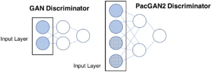
How to pack a discriminator. Note that there are many ways to change the discriminator architecture to accept packed input samples. We propose to keep all hidden layers of the discriminator exactly the same as the mother architecture, and only increase the number of nodes in the input layer by a factor ofm. For example, in Figure 3.1, suppose we start with a mother architecture in which the discriminator is a fully-connected feed-forward network. Here, each sample X lies in a space of dimension p = 2, so the input layer has two nodes. Now, under PacGAN2, we would multiply the size of the input layer by the packing degree (in this case, two), and the connections to the first hidden layer would be adjusted so that the first two layers remain fully-connected, as in the mother architecture. The grid-patterned

1_{For a list of some popular GANs, we refer to the GAN zoo:}

Figure 3.1: PacGAN(m) augments the input layer by a factor of m. The number of edges between the first two layers are increased accordingly to preserve the connectivity of the mother architecture (typically fully-connected). Packed samples are fed to the input layer in a concatenated fashion; the grid-patterned nodes represent input nodes for the second input sample.

nodes in Figure 3.1 represent input nodes for the second sample.

Similarly, when packing a DCGAN, which uses convolutional neural networks for both the generator and the discriminator, we simply stack the images into a tensor of depth m. For instance, the discriminator for PacDCGAN5 on the MNIST dataset of handwritten images [44] would take an input of size 28_×28_×5, since each individual black-and-white MNIST image is 28_×28 pixels. Only the input layer and the number of weights in the corresponding first convolutional layer will increase in depth by a factor of five. By modifying only the input dimension and fixing the number of hidden and output nodes in the discriminator, we can focus purely on the effects of packing in our numerical experiments in Chapter 4. How to train a packed discriminator. Just as in standard GANs, we train the packed discriminator with a bag of samples from the real data and the generator. However, each minibatch in the stochastic gradient descent now consists of packed samples. Each packed sample is of the form (X1, X2, . . . , Xm, Y), where the label is Y = 1 for real data andY = 0 for generated data, and the m independent samples from either class are jointly treated as a single, higher-dimensional feature (X1, . . . , Xm). The discriminator learns to classify m packed samples jointly. Intuitively, packing helps the discriminator detect mode collapse because lack of diversity is more obvious in a set of samples than in a single sample. Fun-damentally, packing allows the discriminator to observe samples from product distributions, which highlight mode collapse more clearly than unmodified data and generator distribu-tions. We make this statement precise in Chapter 5.

Notice that the computational overhead of PacGAN training is marginal, since only the input layer of the discriminator gains new parameters. Furthermore, we keep all training hyperparameters identical to the mother architecture, including the stochastic gradient de-scent minibatch size, weight decay, learning rate, and the number of training epochs. This

is in contrast with other approaches for mitigating mode collapse that require significant computational overhead and/or delicate hyperparameter selection [17, 16, 14, 2, 18].

Computational complexity. The exact computational complexity overhead of PacGAN (compared to GANs) is architecture-dependent, but can be computed in a straightforward manner. For example, consider a discriminator withwfully-connected layers, each containing

g nodes. Since the discriminator has a binary output, the (w+ 1)th layer has a single node, and is fully connected to the previous layer. We seek the computational complexity of a single minibatch parameter update, where each minibatch contains r samples. Backpropagation in such a network is dominated by the matrix-vector multiplication in each hidden layer, which has complexityO(g2) per input sample, assuming a naive implementation. Hence the overall minibatch update complexity is O(rwg2_{). Now suppose the input layer is expanded}

by a factor ofm. If we keep the same number of minibatch elements, the per-minibatch cost grows to O((w+m)rg2_{). We find that in practice, evenm = 2 orm = 3 give good results.}

CHAPTER 4: EXPERIMENTS

On standard benchmark datasets, we compare PacGAN to several baseline GAN architec-tures, some of which are explicitly proposed to mitigate mode collapse: GAN [3], DCGAN [14], VEEGAN [2], Unrolled GANs [18], and ALI [17]. We also implicitly compare against BIGAN [16], which is conceptually identical to ALI. To isolate the effects of packing, we make minimal choices in the architecture and hyperparameters of our packing implemen-tation. For each experiment, we evaluate packing by taking a standard, baseline GAN implementation that wasnot designed to prevent mode collapse, and adding packing in the discriminator. In particular, our goal for this Chapter is to reproduce experiments from existing literature, apply the packing framework to the simplest GAN among those in the baseline, and showcase how packing affects the performance.

Metrics. For consistency with prior work, we measure several previously-used metrics. On datasets with clear, known modes (e.g., Gaussian mixtures, labelled datasets), prior papers have counted the number of modes that are produced by a generator [16, 18, 2]. In labelled datasets, this number can be evaluated using a third-party trained classifier that classifies the generated samples [14]. In Gaussian Mixture Models (GMMs), for example in [2], a mode is considered lost if there is no sample in the generated test data withinxstandard deviations from the center of that mode. In [2],xis set to be three for 2D-ring and 2D-grid, and ten for 1200D-synthetic. A second metric used in [2] is thenumber of high-quality samples, which is the proportion of the samples that are withinxstandard deviation from the center of a mode. Finally, the reverse Kullback-Leibler divergence over the modes has been used to measure the quality of mode collapse as follows. Each of the generated test samples is assigned to its closest mode; this induces an empirical, discrete distribution with an alphabet size equal to the number of observed modes in the generated samples. A similar induced discrete distribution is computed from the real data samples. The reverse KL divergence between the induced distribution from generated samples and the induced distribution from the real samples is used as a metric. Each of these three metrics has shortcomings—for example, the number of observed modes does not account for class imbalance among generated modes, and all of these metrics only work for datasets with known modes. Defining an appropriate metric for evaluating GANs is an active research topic [35, 36, 37].

Datasets. We use a number of synthetic and real datasets for our experiments, all of which have been studied or proposed in prior work. The 2D-ring [2] is a mixture of eight two-dimensional spherical Gaussians with means (cos((2π/8)i),sin((2π/8)i)) and variances 10−4

in each dimension for i _{∈ {}1, . . . ,8_}. The 2D-grid [2] is a mixture of 25 two-dimensional spherical Gaussians with means (₋4 + 2i,₋4 + 2j) and variances 0.0025 in each dimension for i, j _{∈ {}0,1,2,3,4_}.

To examine real data, we use the MNIST dataset [44], which consists of 70,000 images of handwritten digits, each 28_×28 pixels. Unmodified, this dataset has 10 modes, one for each digit. As done in Mode-regularized GANs [19], Unrolled GANs [18] and VEEGAN [2], we augment the number of modes by stacking the images. That is, we generate a new dataset of 128,000 images, in which each image consists of three randomly-selected MNIST images that are stacked into a 28_×28_×3 image in RGB. This new dataset has (with high probability) 1000 = 10_×10_×10 modes. We refer to this as the stacked MNISTdataset.

4.1 SYNTHETIC DATA EXPERIMENTS FROM VEEGAN [2]

Our first experiment evaluates the number of modes and the number of high-quality sam-ples for the 2D-ring and the 2D-grid. Results are reported in Table 4.1. The first four rows are copied directly from Table 1 in [2]. The last three rows contain our own implemen-tation of PacGANs. We do not make any choices in the hyper-parameters, the generator architecture, the discriminator architecture, and the loss. Our implementation attempts to reproduce the VEEGAN architecture to the best of our knowledge, as described below.

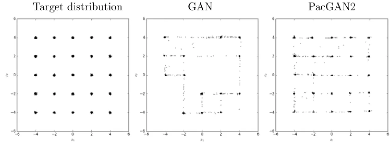
Target distribution GAN PacGAN2

Figure 4.1: Scatter plot of the 2D samples from the true distribution (left) of 2D-grid and the learned generators using GAN (middle) and PacGAN2 (right). PacGAN2 captures all of the 25 modes.

Architecture and hyper-parameters. All of the GANs we implemented in this ex-periment use the same overall architecture, which is chosen to match the architecture in

VEEGAN’s code [2]. The generators have two hidden layers, 128 units per layer with ReLU activation, trained with batch normalization [45]. The input noise is a two dimensional spherical Gaussian with zero mean and unit variance. The discriminator has one hidden layer, 128 units on that layer. The hidden layer uses LinearMaxout with 5 maxout pieces, and no batch normalization is used in the discriminator.

We train each GAN with 100,000 total samples, and a mini-batch size of 100 samples; train-ing is run for 200 epochs. The discriminator’s loss function is log(1 + exp(₋D(real data))) + log(1+exp(D(generated data))), except for VEEGAN which has an additional regularization term. The generator’s loss function is

log(1 + exp(D(real data))) + log(1 + exp(₋D(generated data))).

Adam [46] stochastic gradient descent is applied with the generator weights and the dis-criminator weights updated once per mini-batch. At testing, we use 2500 samples from the learned generator for evaluation. Each metric is evaluated and averaged over 10 trials.

2D-ring 2D-grid

Modes high quality Modes high quality

(Max 8) samples (Max 25) samples

GAN [3] 1.0 99.30 % 3.3 0.5 % ALI [17] 2.8 0.13 % 15.8 1.6 % Unrolled GAN [18] 7.6 35.60 % 23.6 16.0 % VEEGAN [2] 8.0 52.90 % 24.6 40.0 % PacGAN2 (ours) 8.0_±0.0 78.5_±7.7 % 24.6_±0.9 65.8_±13.4 % PacGAN3 (ours) 8.0_±0.0 84.0_±6.1 % 24.9_±0.3 71.4_±13.8 % PacGAN4 (ours) 8.0_±0.0 82.7_±11.3 % 25.0_±0.0 76.0_±7.1 % Table 4.1: Two measures of mode collapse proposed in [2] for two synthetic mixtures of Gaussians: number of modes captured by the generator and percentage of high quality samples. Our results are averaged over 10 trials shown with the standard error.

Results. Table 4.1 shows that PacGAN outperforms or matches the baseline schemes, both in the number of modes captured and the percentage of high quality samples. As expected, increasing the degreem of packing seems to increase the average number of modes found, though the increases are marginal for easy tasks. In the 2D grid and ring, we find that PacGAN slightly outperforms VEEGAN, but the proposed datasets seem not to be challenging enough to highlight meaningful differences. However, one can clearly see the gain of packing by comparing the GAN in the first row (which is the mother architecture)

and PacGANs in the last rows. The simple change we make to the mother architecture according to the principle of packing makes a significant difference in performance, and the overhead of changes made to the mother architecture are minimal compared to the baselines [17, 18, 2].

Note that maximizing the number of high-quality samples is not necessarily indicative of a good generative model. First, we expect some fraction of probability mass to lie outside the “high-quality” boundary, and that fraction increases with the dimensionality of the dataset. For reference, we find empirically that the expected fraction of high-quality samples in the true data distribution for the 2D ring and grid are both 98.9%, which corresponds to the theoretical ratio for a single 2D Gaussian. These values are higher than the fractions found by PacGAN, indicating room for improvement. However, a generative model could output 100% high-quality points by learning very few modes (as is the case for GANs in the 2D ring in Table 4.1).

Note that our goal is not to compete with the baselines of ALI, Unrolled GAN, and VEE-GAN, but to showcase the improvement that can be obtained with packing. In this spirit, we can easily apply our framework to other baselines and test “PacALI”, “PacUnrolledGAN”, and “PacVEEGAN”. In fact, we expect that most GAN architectures can be packed to im-prove sample quality. However, for these benchmark tests, we see that packing the simplest GAN is sufficient.

4.2 STACKED MNIST EXPERIMENTS

In our next experiments, we evaluate mode collapse on the stacked MNIST dataset (de-scribed at the beginning of Chapter 4). These experiments are direct comparisons to anal-ogous experiments in VEEGAN [2] and Unrolled GANs [18]. For these evaluations, we generate 26,000 samples from the generator. Each of the three channels in each sample is classified by a pre-trained third-party MNIST classifier, and the resulting three digits deter-mine which of the 1,000 modes the sample belongs to. We measure the number of modes captured, as well as the KL divergence between the generated distribution over modes and the expected true one (i.e., a uniform distribution over the 1,000 modes).

Hyperparameters. For these experiments, we train each GAN on 128,000 samples, with a mini-batch size of 64. The generator’s loss function is -log(D(generated data)), and the discriminator’s loss function is -log(D(real data))-log(1-D(generated data)). We update the generator parameters twice and the discriminator parameters once in each mini-batch, and train the generators over 50 epochs. For testing, we generate 26,000 samples, and evaluate

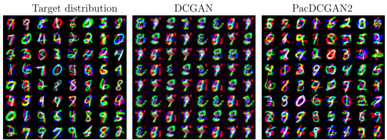
Target distribution DCGAN PacDCGAN2

Figure 4.2: True distribution (left), DCGAN generated samples (middle), and PacDCGAN2 generated samples (right) from the stacked-MNIST dataset show PacDCGAN2 captures more diversity while producing sharper images.

the empirical KL divergence and number of modes covered. Finally, we average these values over 10 runs of the entire pipeline.

4.2.1 VEEGAN [2] Experiment

In this experiment, we replicate Table 2 from [2], which measured the number of observed modes in a generator trained on the stacked MNIST dataset, as well as the KL divergence of the generated mode distribution.

Architecture. In line with prior work [2], we used a DCGAN-like architecture for these experiments, which is based on the code at https://github.com/carpedm20/

DCGAN-tensorflow. In particular, the generator and discriminator architectures are as

fol-lows:

Generator:

layer #outputs kernel size stride activation Input: z _∼U(₋1,1)100 100

Fully connected 2*2*512 ReLU

Transposed Convolution 4*4*256 5*5 2 ReLU Transposed Convolution 7*7*128 5*5 2 ReLU Transposed Convolution 14*14*64 5*5 2 ReLU Transposed Convolution 28*28*3 5*5 2 Tanh

Discriminator (for PacDCGANm):

layer #outputs kernel size stride BN activation Input: x_∼pm

data 28*28*(3*m)

Convolution 14*14*64 5*5 2 LeakyReLU

Convolution 7*7*128 5*5 2 Yes LeakyReLU

Convolution 4*4*256 5*5 2 Yes LeakyReLU

Convolution 2*2*512 5*5 2 Yes LeakyReLU

Fully connected 1 Sigmoid

Results. Results are shown in Table 4.2. Again, the first four rows are copied directly from [2]. The last three rows are computed using a basic DCGAN, with packing in the discriminator. We find that packing gives good mode coverage, reaching all 1,000 modes in every trial. Given a DCGAN that can capture at most 99 modes on average (our mother architecture), the principle of packing, which is a small change in the architecture, is able to improve performance to capture all 1,000 modes. Again we see that packing the simplest DCGAN is sufficient to fully capture all the modes in this benchmark tests, and we do not pursue packing more complex baseline architectures. Existing approaches to mitigate mode collapse, such as ALI, Unrolled GANs, and VEEGAN, are not able to capture as many modes. Stacked MNIST Modes (Max 1000) KL DCGAN [34] 99.0 3.40 ALI [17] 16.0 5.40 Unrolled GAN [18] 48.7 4.32 VEEGAN [2] 150.0 2.95 PacDCGAN2 (ours) 1000.0_±0.0 0.06_±0.01 PacDCGAN3 (ours) 1000.0_±0.0 0.06_±0.01 PacDCGAN4 (ours) 1000.0_±0.0 0.07_±0.01

Table 4.2: Two measures of mode collapse proposed in [2] for the stacked MNIST dataset: number of modes captured by the generator and reverse KL divergence over the generated mode distribution.

Note that other classes of GANs may also be able to learn most or all of the modes if tuned properly. For example, [18] reports that regular GANs can learn all 1,000 modes even without unrolling if the discriminator is large enough, and if the discriminator is half the

size of the generator, unrolled GANs recover up to 82% of the modes when the unrolling parameter is increased to 10. To explore this effect, we conduct further experiments on unrolled GANs in Chapter 4.2.2.

4.2.2 Unrolled GAN [18] Experiment

This experiment is designed to replicate Table 1 from Unrolled GANs [18]. Unrolled GANs exploit the observation that iteratively updating discriminator and generator model parameters can contribute to training instability. To mitigate this, they update model parameters by computing the loss function’s gradient with respect to k _≥ 1 sequential discriminator updates, where k is called the unrolling parameter. [18] reports that unrolling improves mode collapse as k increases, at the expense of greater training complexity.

Unlike Chapter 4.2.1, which reported a single metric for unrolled GANs, this experiment studies the effect of the unrolling parameter and the discriminator size on the number of modes learned by a generator. The key differences between these trials and the unrolled GAN row in Table 4.2 are threefold: (1) the unrolling parameters are different, (2) the discriminator sizes are different, and (3) the generator and discriminator architectures are chosen according to Appendix E in [18].

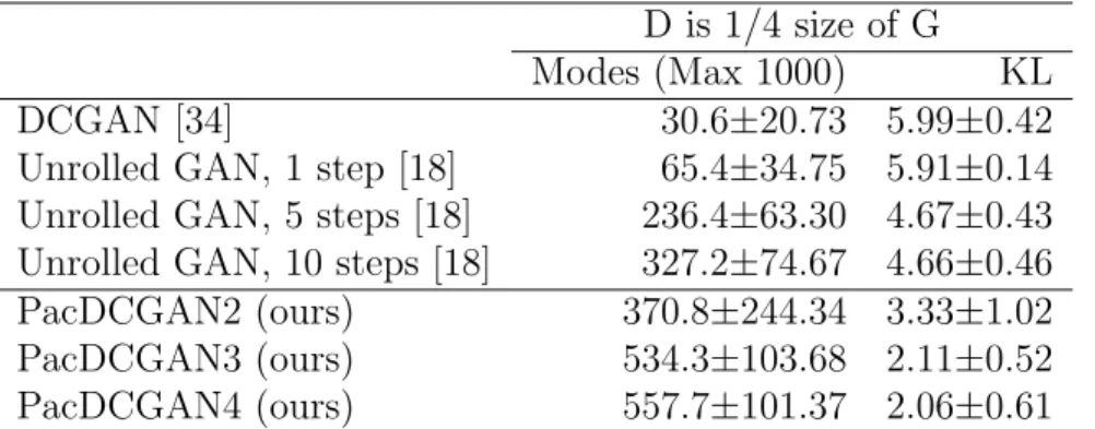
Results. Our results are reported in Tables 4.3 and 4.4. The first four rows are copied from [18]. As before, we find that packing seems to increase the number of modes covered. Additionally, in both experiments, PacDCGAN finds more modes on average than Unrolled GANs withk = 10, with lower reverse KL divergences between the mode distributions. This suggests that packing has a more pronounced effect than unrolling. However, note that the standard error for PacDCGANs is larger than that reported in [18]; this may be due to our relatively small sample size of 10.

D is 1/4 size of G

Modes (Max 1000) KL

DCGAN [34] 30.6_±20.73 5.99_±0.42

Unrolled GAN, 1 step [18] 65.4_±34.75 5.91_±0.14 Unrolled GAN, 5 steps [18] 236.4_±63.30 4.67_±0.43 Unrolled GAN, 10 steps [18] 327.2_±74.67 4.66_±0.46 PacDCGAN2 (ours) 370.8_±244.34 3.33_±1.02 PacDCGAN3 (ours) 534.3_±103.68 2.11_±0.52 PacDCGAN4 (ours) 557.7_±101.37 2.06_±0.61 Table 4.3: Modes covered and KL divergence for unrolled GANs as compared to PacDCGANs for various unrolling parameters, discriminator sizes, and the degree of packing.

D is 1/2 size of G

Modes (Max 1000) KL

DCGAN [34] 628.0_±140.9 2.58_±0.75

Unrolled GAN, 1 step [18] 523.6_±55.77 2.44_±0.26 Unrolled GAN, 5 steps [18] 732.0_±44.98 1.66_±0.09 Unrolled GAN, 10 steps [18] 817.4_±37.91 1.43_±0.12 PacDCGAN2 (ours) 877.1_±51.96 0.99_±0.13 PacDCGAN3 (ours) 851.6_±98.60 1.02_±0.34 PacDCGAN4 (ours) 896.0_±72.83 0.82_±0.25 Table 4.4: Modes covered and KL divergence for unrolled GANs as compared to PacDCGANs for various unrolling parameters, discriminator sizes, and the degree of packing.

CHAPTER 5: THEORETICAL ANALYSES OF PACGAN

In this chapter, we propose a formal and natural mathematical definition of mode collapse, which abstracts away domain-specific details (e.g. images vs. time series). For a target distributionP and a generator distributionQ, this definition describes mode collapse through a two-dimensional representation of the pair (P, Q) as a region.

Mode collapse is a phenomenon commonly reported in the GAN literature [32, 15, 39, 47, 38], which can refer to two distinct concepts: (i) the generative model loses some modes that are present in the samples of the target distribution. For example, despite being trained on a dataset of animal pictures that includes lizards, the model never generates images of lizards. (ii) Two distant points in the code vectorZ are mapped to the same or similar points in the sample space X. For instance, two distant latent vectorsz1 and z2 map to the same picture

of a lizard [32]. Although these phenomena are different, and either one can occur without the other, they are generally not explicitly distinguished in the literature, and it has been suggested that the latter may cause the former [32]. In this work, we focus on the former notion, as it does not depend on how the generator maps a code vector Z to the sample X, and only focuses on the quality of the samples generated. In other words, we assume here that two generative models with the same marginal distribution over the generated samples should not be treated differently based on how random code vectors are mapped to the data sample space. The second notion of mode collapse would differentiate two such architectures, and is beyond the scope of this work. The proposed region representation relies purely on the properties of the generated samples, and not on the generator’s mapping between the latent and sample spaces.

We analyze how the proposed idea of packing changes the training of the generator. We view the discriminator’s role as providing a surrogate for a desired loss to be minimized— surrogate in the sense that the actual desired losses, such as Jensen-Shannon divergence or total variation distances, cannot be computed exactly and need to be estimated. Consider the standard GAN discriminator with a cross-entropy loss:

min

G maxD EX∼P[log(D(X))]−EG(Z)∼Q[log(1−D(G(Z)))]

| {z } ' DKL PkP+₂Q +DKL QkP+₂Q , (5.1)

where the maximization is over the family of discriminators (or the discriminator weights, if the family is a neural network of a fixed architecture), the minimization is over the family of generators, and X is drawn from the distribution P of the real data, Z is drawn from

the distribution of the code vector, typically a low-dimensional Gaussian, and we denote the resulting generator distribution asG(Z)_∼Q. The role of the discriminator under this GAN scenario is to provide the generator with an approximation (or a surrogate) of a loss, which in the case of cross entropy loss turns out to be the Jensen-Shannon divergence, defined as

DKL(Pk(P +Q)/2) +DKL(Qk(P +Q)/2), whereDKL(·) is the Kullback-Leibler divergence.

This follows from the fact that, if we search for the maximizing discriminator over the space of all functions, the maximizer turns out to beD(X) =P(X)/(P(X) +Q(X)) [3]. In practice, we search over some parametric family of discriminators, and we can only compute sample average of the losses. This provides an approximation of the Jensen-Shannon divergence betweenP andQ. The outer minimization over the generator tries to generate samples such that they are close to the real data in this (approximate) Jensen-Shannon divergence, which is one measure of how close the true distribution P and the generator distribution Qare.

In this Chapter, we show a fundamental connection between the principle of packing and mode collapse in GAN. We provide a complete understanding of how packing changes the loss as seen by the generator, by focusing on (as we did to derive the Jensen-Shnnon divergence above) (a) the optimal discriminator over a family of all measurable functions; (b) the population expectation; and (c) the 0-1 loss function of the form:

max

D EX∼P[I(D(X))] +EG(Z)∼Q[1−I(D(G(Z)))] subject to D(X)_{∈ {}0,1_}.

The first assumption allows us to bypass the specific architecture of the discriminator used, which is common when analyzing neural network based discriminators (e.g. [48]). The second assumption can be potentially relaxed and the standard finite sample analysis can be applied to provide bounds similar to those in our main results in Theorems 5.1, 5.2, and 5.3. The last assumption gives a loss of the total variation distance dTV(P, Q), supS⊆X{P(S)−Q(S)} over the domain _X. This follows from the fact that (e.g. [32]),

sup D EX∼P[I(D(X))] +EG(Z)∼Q[1−I(D(G(Z)))] = sup S P(S) + 1₋Q(S) = 1 +dTV(P, Q).

This discriminator provides (an approximation of) the total variation distance, and the generator tries to minimize the total variation distance

The reason we make this assumption is primarily for clarity and analytical tractability: total variation distance highlights the effect of packing in a way that is cleaner and easier to understand than if we were to analyze Jensen-Shannon divergence. We discuss this point in more detail in Chapter 5.2. In sum, these three assumptions allow us to focus purely on the impact of packing on the mode collapse of resulting discriminator.

We want to understand how this 0-1 loss, as provided by such a discriminator, changes with the degree of packingm. As packed discriminators see m packed samples, each drawn i.i.d. from one joint class (i.e. either real or generated), we can consider these packed samples as a single sample that is drawn from the product distribution: Pmfor real andQmfor generated. The resulting loss provided by the packed discriminator is therefore dTV(Pm, Qm).

We first provide a formal mathematical definition of mode collapse in Chapter 5.1, which leads to a two-dimensional representation of any pair of distributions (P, Q) as a mode-collapse region. This region representation provides not only conceptual clarity regarding mode collapse, but also proof techniques that are essential to proving our main results on the fundamental connections between the strength of mode collapse in a pair (P, Q) and the loss

dTV(Pm, Qm) seen by a packed discriminator (Chapter 5.2). The proofs of these results are

provided in Chapter 6. In Chapter 5.2.1, we show that the proposed mode collapse region is equivalent to what is known as the hypothesis testing region for type I and type II errors in binary hypothesis testing. This allows us to use strong mathematical techniques from binary hypothesis testing including the data processing inequality and the reverse data processing inequalities.

5.1 MATHEMATICAL DEFINITION OF MODE COLLAPSE AS A TWO-DIMENSIONAL REGION

Although no formal and agreed-upon definition of mode collapse exists in the GAN lit-erature, mode collapse is declared for a multimodal target distribution P if the generator

Q assigns a significantly smaller probability density in the regions surrounding a particular subset of modes. One major challenge in addressing such a mode collapse is that it involves the geometry of P: there is no standard partitioning of the domain respecting the modu-lar topology of P, and even heuristic partitions are typically computationally intractable in high dimensions. Hence, we drop this geometric constraint, and introduce a purely analytical definition.

Definition 5.1. A target distribution P and a generator Q exhibit (ε, δ)-mode collapse for some 0_≤ε < δ_≤1 if there exists a set S _{⊆ X} such that P(S)_≥δ and Q(S)_≤ε.

This definition provides a formal measure of mode collapse for a targetP and a generator

Q; intuitively, larger δ and smaller ε indicate more severe mode collapse. That is, if a large portion of the target P(S) _≥ δ in some set S in the domain _X is missing in the generator

Q(S)_≤ε, then we declare (ε, δ)-mode collapse.

A key observation is that two pairs of distributions can have the same total variation distance while exhibiting very different mode collapse patterns. To see this, consider a toy example in Figure 5.1, with a uniform target distribution P = U([0,1]) over [0,1]. Now consider all generators at a fixed total variation distance of 0.2 from P. We compare the intensity of mode collapse for two extreme cases of such generators. Q1 = U([0.2,1]) is

uniform over [0.2,1] and Q2 = 0.6U([0,0.5]) + 1.4U([0.5,1]) is a mixture of two uniform

distributions, as shown in Figure 5.1. They are designed to have the same total variations distance, i.e. dTV(P, Q1) = dTV(P, Q2) = 0.2, but Q1 exhibits an extreme mode collapse as

the whole probability mass in [0,0.2] is lost, whereas Q2 captures a more balanced deviation

fromP.

Definition 5.1 captures the fact that Q1 has more mode collapse than Q2, since the pair

(P, Q1) exhibits (ε = 0, δ= 0.2)-mode collapse, whereas the pair (P, Q2) exhibits only (ε=

0.12, δ = 0.2)-mode collapse, for the same value ofδ = 0.2. However, the appropriate way to precisely represent mode collapse (as we define it) is to visualize it through a two-dimensional region we call the mode collapse region. For a given pair (P, Q), the corresponding mode collapse region _R(P, Q) is defined as the convex hull of the region of points (ε, δ) such that (P, Q) exhibit (ε, δ)-mode collapse, as shown in Figure 5.1.

R(P, Q) _, conv

(ε, δ)δ > ε and (P, Q) has (ε, δ)-mode collapse

, (5.2) where conv(_·) denotes the convex hull. This definition of region is fundamental in the sense that it is a sufficient statistic that captures the relations between P and Q. This assertion is made precise in Chapter 5.2.1 by making a strong connection between the mode collapse region and the type I and type II errors in binary hypothesis testing. That connection allows us to prove a sharp result on how the loss, as seen by the discriminator, evolves under PacGAN in Chapter 6. For now, we can use this region representation of a given target-generator pair to detect the strength of mode collapse occurring for a given target-generator.

Typically, we are interested in the presence of mode collapse with a smallε and a much larger δ; this corresponds to a sharply-increasing slope near the origin (0,0) in the mode collapse region. For example, the middle panel in Figure 5.1 depicts the mode collapse region (shaded in gray) for a pair of distributions (P, Q1) that exhibit significant mode collapse;

same region for a pair of distributions (P, Q2) that do not exhibit strong mode collapse,

resulting a region with a much gentler slope at (0,0).

1 1 1.25 0.2 1 1 1 1 0.6 1.4 0.5 P Q1 Q2 0 0.5 1 0 0.5 1 R(P, Q1) ε δ 0 0.5 1 0 0.5 1 R(P, Q2) ε δ

Figure 5.1: A formal definition of (ε, δ)-mode collapse and its accompanying region

representation captures the intensity of mode collapse for generatorsQ1 with mode collapse

and Q2 which does not have mode collapse, for a toy example distributions P, Q1, and Q2

shown on the left. The region of (ε, δ)-mode collapse that is achievable is shown in grey. Similarly, if the generator assigns a large probability mass compared to the target distri-bution on a subset, we call it a mode augmentation, and give a formal definition below. Definition 5.2. A pair of a target distribution P and a generator Q has an (ε, δ)-mode augmentation for some 0 _≤ ε < δ _≤1 if there exists a set S _{⊆ X} such that Q(S) _≥ δ and

P(S)_≤ε.

Note that we distinguish mode collapse and augmentation strictly here, for analytical purposes. In GAN literature, both collapse and augmentation contribute to the observed “mode collapse” phenomenon, which loosely refers to the lack of diversity in the generated samples.

5.2 EVOLUTION OF THE REGION UNDER PRODUCT DISTRIBUTIONS

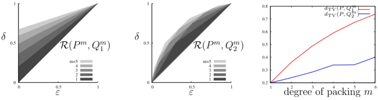
The toy example generatorsQ1 and Q2 from Figure 5.1 could not be distinguished using

only their total variation distances from P, despite exhibiting very different mode collapse properties. This suggests that the original GAN (with 0-1 loss) may be vulnerable to mode collapse, as it has no way to distinguish distributions in which mode collapse does or does not happen. We prove in Theorem 5.2 that a discriminator that packs multiple samples together can distinguish mode-collapsing generators. Intuitively, m packed samples are effectively drawn from the product distributions Pm and Qm. We show in this section that

there is a fundamental connection between the strength of mode collapse of (P, Q) and the loss as seen by the packed discriminator dTV(Pm, Qm).

Intuition via toy examples. Concretely, consider the example from the previous section and recall that Pm _{denote the product distribution resulting from packing together m} inde-pendent samples from P. Figure 5.2 illustrates how the mode collapse region evolves over

m, the degree of packing. This evolution highlights a key insight: the region _R(Pm_{, Q}m

1 )

of a mode-collapsing generator expands much faster as m increases compared to the region R(Pm, Qm₂ ) of a non-mode-collapsing generator. This implies that the total variation dis-tance of (P, Q1) increases more rapidly as we pack more samples, compared to (P, Q2). This

follows from the fact that the total variation distance between P and the generator can be determined directly from the upper boundary of the mode collapse region (see Chapter 5.2.1 for the precise relation). In particular, a larger mode collapse region implies a larger total variation distance between P and the generator. The total variation distances dTV(P, Qm1 )

and dTV(P, Qm2 ), which were explicitly chosen to be equal at m = 1 in our example, grow

farther apart with increasing m, as illustrated in the right figure below. This implies that if we use a packed discriminator, the mode-collapsing generator Q1 will be heavily penalized

for having a larger loss, compared to the non-mode-collapsing Q2.

0 0.5 1 0 0.5 1 m=5 4 3 2 1 R(Pm_{, Q}m 1 ) ε δ 0 0.5 1 0 0.5 1 m=5 4 3 2 1 R(Pm_{, Q}m 2) ε δ 0.2 0.3 0.4 0.5 0.6 0.7 0.8 1 2 3 4 5 6 degree of packing m dTV(P, Qm1) dTV(P, Qm2)

Figure 5.2: Evolution of the mode collapse region over the degree of packing m for the two toy examples from Figure 5.1. The region of the mode-collapsing generator Q1 expands

faster than the non-mode-collapsing generator Q2 when discriminator inputs are packed (at

m= 1 these examples have the same TV distances). This causes a discriminator to penalize mode collapse as desired.

Evolution of total variation distances. In order to generalize the intuition from the above toy examples, we first analyze how the total variation evolves for the set of all pairs (P, Q) that have the same total variation distanceτ when unpacked (i.e., whenm= 1). The solutions to the following optimization problems give the desired upper and lower bounds,

respectively, on total variation distance for any distribution pair in this set with a packing degree of m: min P,Q dTV(P m , Qm) max P,Q dTV(P m , Qm) (5.3) subject to dTV(P, Q) = τ subject to dTV(P, Q) = τ ,

where the maximization and minimization are over all probability measures P and Q. We give the exact solution in Theorem 5.1, which is illustrated pictorially in Figure 5.3 (left). Theorem 5.1. For all 0_≤τ _≤1and a positive integer m, the solution to the maximization in (5.3) is 1₋(1₋τ)m_{, and the solution to the minimization in (5.3) is}

L(τ, m) _, min 0≤α≤1−τ dTV Pinner(α)m, Qinner(α, τ)m , (5.4)

wherePinner(α)m andQinner(α, τ)m are them-th order product distributions of binary random

variables distributed as Pinner(α) = h 1₋α, α i , (5.5) Qinner(α, τ) = h 1₋α₋τ, α+τ i . (5.6)

Although this is a simple statement that can be proved in several different ways, we introduce in Chapter 6 a novel geometric proof technique that critically relies on the proposed mode collapse region. This particular technique will allow us to generalize the proof to more complex problems involving mode collapse in Theorem 5.2, for which other techniques do not generalize. Note that the claim in Theorem 5.1 has nothing to do with mode collapse. Still, we use the mode collapse region definition purely as a proof technique for this claim.

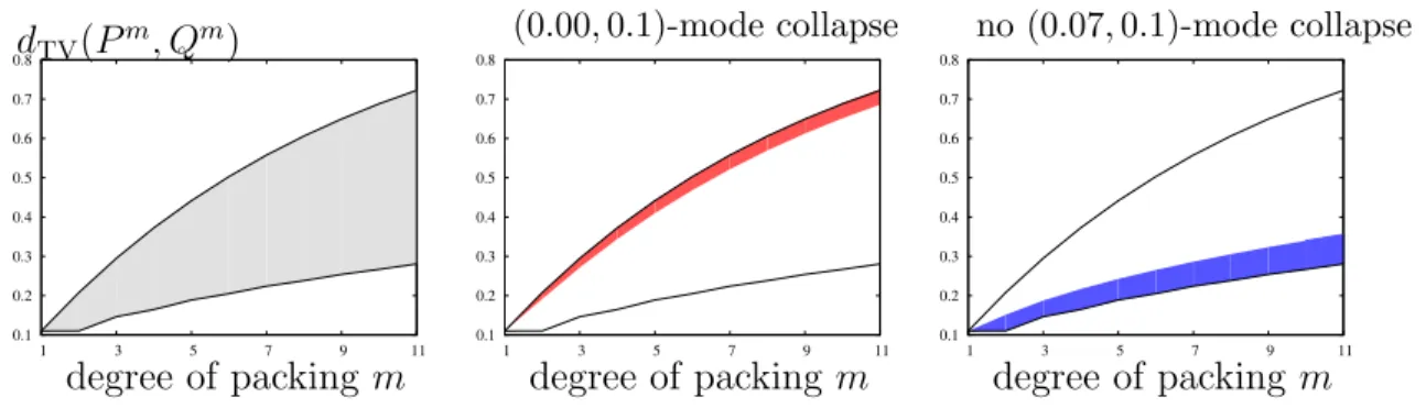
For any given value ofτandm, the bounds in Theorem 5.1 are easy to evaluate numerically, as shown below in the left panel. Within this achievable range, some pairs (P, Q) have rapidly increasing total variation, occupying the upper part of the region (shown in red, middle panel of Figure 5.3), and some pairs (P, Q) have slowly increasing total variation, occupying the lower part as shown in blue in the right panel in Figure 5.3. In particular, the evolution of the mode-collapse region of a pair of m-th power distributions _R(Pm, Qm) is fundamentally connected to the strength of mode collapse in the original pair (P, Q). This means that for a mode-collapsed pair (P, Q1), the mth-power distribution will exhibit a different total

variation distance evolution than a non-mode-collapsed pair (P, Q2). As such, these two pairs

class of mode-collapsing and non-mode-collapsing generators is challenging, as it depends on the target P and the generator Q, each of which can be a complex high dimensional distribution, like natural images. The proposed region interpretation, endowed with the hypothesis testing interpretation and the data processing inequalities that come with it, is critical: it enables the abstraction of technical details and provides a simple and tight proof based on geometric techniques on two-dimensional regions.

0.1 0.2 0.3 0.4 0.5 0.6 0.7 0.8 1 3 5 7 9 11 dTV(Pm, Qm) degree of packing m 0.1 0.2 0.3 0.4 0.5 0.6 0.7 0.8 1 3 5 7 9 11 (0.00,0.1)-mode collapse degree of packing m 0.1 0.2 0.3 0.4 0.5 0.6 0.7 0.8 1 3 5 7 9 11 no (0.07,0.1)-mode collapse degree of packing m

Figure 5.3: The range of dTV(Pm, Qm) achievable by pairs with dTV(P, Q) = τ, for a choice

of τ = 0.11, defined by the solutions of the optimization (5.3) provided in Theorem 5.1 (left panel). The range ofdTV(Pm, Qm) achievable by those pairs that also have

(ε= 0.00, δ= 0.1)-mode collapse (middle panel). A similar range achievable by pairs of distributions that do not have (ε= 0.07, δ= 0.1)-mode collapse or (ε = 0.07, δ = 0.1)-mode augmentation (right panel). Pairs (P, Q) with strong mode collapse occupy the top region (near the upper bound) and the pairs with weak mode collapse occupy the bottom region (near the lower bound).

Evolution of total variation distances with mode collapse. We analyze how the total variation evolves for the set of all pairs (P, Q) that have the same total variations distances

τ when unpacked, with m = 1, and have (ε, δ)-mode collapse for some 0 _≤ ε < δ _≤ 1. The solution of the following optimization problem gives the desired range of total variation distances: min P,Q dTV(P m , Qm) max P,Q dTV(P m , Qm) (5.7) subject to dTV(P, Q) = τ subject to dTV(P, Q) =τ

(P, Q) has (ε, δ)-mode collapse (P, Q) has (ε, δ)-mode collapse,

where the maximization and minimization are over all probability measures P and Q, and the mode collapse constraint is defined in Definition 5.1. (ε, δ)-mode collapsing pairs have total variation at leastδ₋εby definition, and when τ < δ₋ε, the feasible set of the above

optimization is empty. Otherwise, the next theorem establishes that mode-collapsing pairs occupy the upper part of the total variation region; that is, total variation increases rapidly as we pack more samples together (Figure 5.3, middle panel). This follows from the fact that any pair (P, Q) with total variation distance τ _≥ δ₋ inherently exhibits (δ, ) mode collapse. One implication is that distribution pairs (P, Q) at the top of the total variation evolution region are those with the strongest mode collapse. Another implication is that a pair (P, Q) with strong mode collapse (i.e., with largerδand smallerεin the constraint) will be penalized more under packing, and hence a generator minimizing an approximation of

dTV(Pm, Qm) will be unlikely to select a distribution that exhibits such strong mode collapse.

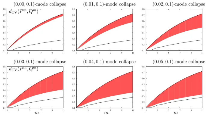
Theorem 5.2. For all 0 _≤ ε < δ _≤ 1 and a positive integer m, if 1_≥ τ _≥ δ₋ε then the solution to the maximization in (5.7) is 1₋(1₋τ)m_{, and the solution to the minimization} in (5.7) is L1(ε, δ, τ, m) , min n min 0≤α≤1− τ δ δ−ε dTV Pinner1(δ, α)m, Qinner1(ε, α, τ)m , min 1−τ δ δ−ε≤α≤1−τ dTV Pinner2(α)m, Qinner2(α, τ)m o , (5.8) wherePinner1(δ, α)m,Qinner1(ε, α, τ)m,Pinner2(α)m, andQinner2(α, τ)mare them-th order

prod-uct distributions of discrete random variables distributed as

Pinner1(δ, α) = h δ, 1₋α₋δ, α i , (5.9) Qinner1(ε, α, τ) = h ε, 1₋α₋τ ₋ε, α+τ i , (5.10) Pinner2(α) = h 1₋α, α i , (5.11) Qinner2(α, τ) = h 1₋α₋τ, α+τ i . (5.12)

If τ < δ₋ε, then the optimization in (5.7) has no solution and the feasible set is an empty set.

A proof of this theorem is provided in Chapter 6.1.1, which critically relies on the proposed mode collapse region representation of the pair (P, Q), and the celebrated result by Blackwell from [1]. The solutions in Theorem 5.2 can be numerically evaluated for any given choices of (ε, δ, τ) as we show in Figure 5.4.

Analogous results to the above theorem can be shown for pairs (P, Q) that exhibit (, δ) mode augmentation (as opposed to mode collapse). These results are omitted for brevity, but the results and analysis are straightforward extensions of the proofs for mode collapse.