The Relation between Irradiation Assisted Stress Corrosion Cracking and Dislocation Channeling: The Role of Slip Interaction at the Grain Boundary.

(1)

THE RELATION BETWEEN IRRADIATION ASSISTED STRESS CORROSION CRACKING AND DISLOCATION CHANNELING: THE ROLE OF SLIP

INTERACTION AT THE GRAIN BOUNDARY

by

Michael David McMurtrey

A dissertation submitted in partial fulfillment of the requirements for the degree of

Doctor of Philosophy

(Nuclear Engineering and Radiological Sciences) in The University of Michigan

2014

Doctoral Committee:

Professor Gary S. Was, Chairman Professor Michael Atzmon

Associate Professor Samantha H. Daly Associate Research Scientist Kai Sun

(2)

(3)

ii To my family

(4)

iii

ACKNOWLEDGEMENTS

I would like to thank my advisor, Dr. Gary S. Was, for his guidance throughout my doctoral program, and for the time he dedicated to assist me in completing this thesis. His assistance has been greatly appreciated in our discussions on both the research itself, as well as all written works that came from this research. I would also like to thank the members of my dissertation committee, Dr. Atzmon, Dr. Daly and Dr. Sun, for their willingness to serve on my doctoral committee and provide assistance in this work.

I would like to thank my colleagues for their assistance throughout my years in the doctoral program. My start in graduate school was assisted greatly by the training and encouragement provided by Elaine West, Deepak Kumar, Pantip Ampornrat, Janelle Wharry and Anne Campbell. Over the years, I benefited greatly from the encouragement and discussions with Cheng Xu, Kale Stephenson, Tyler Moss, Gocke Gulsoy, Stephen Raimen, Shyam Dwaraknath, Liz Getto, Justin Hesterberg and Anthony Monterrosa.

A special thanks to Zhijie (George) Jiao for his assistance in all areas of my research. I am grateful for the help I received from Ovidiu Toader and Fabian Naab at the Michigan Ion Beam Laboratory, as well as the continual support and assistance I received from Alex Flick.

(5)

iv

Finally, I would like to thank my family. My parents, Gary and Sheri, as well as my siblings (Brian, Daniel, Erin, Kristi, Julie and Kelly), for their unconditional support and encouragement over the years. My wife, Kate McMurtrey, for her love and patience even in times of stress and for providing me with encouragement and optimism throughout this endeavor.

This work was supported by the U.S. Department of Energy, Office of Basic Energy Sciences, under grant DE-FG02-08ER46525

(6)

v

LIST OF FIGURES

Figure 2.1 Effects of nitrogen content and temperature on yield strength of a 26 Cr, 31 Ni austenitic steel [101]. ... 48 Figure 2.2 Close packed {111} planes in an FCC crystal. ... 49 Figure 2.3 Phase diagram showing percent austenite, ferrite and martensite based on steel composition [18]. ... 50 Figure 2.4 Crack growth rates as a function of water conductivity in 288 °C water with 200ppb oxygen [26]. ... 51 Figure 2.5 Orientation map depicting a section of austenitic stainless steel. ... 52 Figure 2.6 Pole figure demonstration. (a) depicts a unit cell of the crystal, with arrows showing normal to {100} and {111} planes. (b) depicts the stereographic projection of (a), which is the pole figure. ... 53 Figure 2.7 Schematic showing angles used in Eq. 2.1. λ is the angle between the slip direction and the tensile axis, and φ is the angle between the slip plane normal and the tensile axis. ... 54 Figure 2.8 Schmid factor based on crystal orientation in an FCC structure [32]. ... 55 Figure 2.9 Representation of Taylor’s [30] assumption that each grain in a polycrystalline material undergoes the an equivalent deformation as the full macroscopic material. ... 56 Figure 2.10 Grain orientation dependence of the Taylor factor for fcc materials [102]. . 57 Figure 2.11 Depiction of the coincident sites if adjacent lattices from a Σ5 boundary are overlapped on top of each other. ... 58 Figure 2.12 Measured relative energies of [110] tilt boundaries in aluminium. All boundary energies are reference to the 129° boundary. The 70° boundary is equivalent to a (111) twin plane, as would be seen in austenitic steel. [35] . 59 Figure 2.13 Mises equivalent stress distribution from a finite element analysis of a polycrystalline material, showing stress peaks at grain boundaries [40]. ... 60 Figure 2.14 Schematic showing a [111] glide plane and the movement of a perfect dislocation above it from a to c being divided into partials which move from a to b and then to c [103]. ... 61 Figure 2.15 Methods of slip accommodation at a grain boundary [45,47]. ... 62 Figure 2.16 Deformation twinning of copper alloys were tested by Venables [55] and lower SFE materials were found to tend towards lower twinning stresses, resulting in easier deformation twin nucleation. ... 63

(10)

ix

Figure 2.17 Example of deformation: Shape Ψ1 deforms into Ψ2. These shapes are three dimensional and extend into the page. Plane X is depicted within Ψ1, and deforms into plane Y within Ψ2. A point on plane X is described by vector xi, where i has values of 1, 2, and 3, and represent the Cartesian components of x, with 1 being the horizontal component, 2 being the vertical component, and 3 being the component normal to the paper (represented by the ei axis). xi deforms to vector yi by the displacement vector ui(xi) ... 64 Figure 2.18 A dislocation line being pinned by defects, as seen by in a TEM image (left) and as seen using a computer simulation [104]. ... 65 Figure 2.19 Room temperature stress-strain curves for 316 steel irradiated up to 0.78 dpa [72]. ... 66 Figure 2.20 Composition across grain boundary (a), showing major (b) and minor (c) alloying elements. Dashed line in (b) indicates bulk iron concentration [100]. ... 67 Figure 2.21 Slip steps from dislocation channels visible on the surface of a 5 dpa proton irradiated austenitic steel with 21 Cr, 32Ni strained to ~2% in a 288°C argon environment. ... 68 Figure 2.22 (a) Channel width versus resolved shear stress in a 316 SS [72] and (b) channel width versus angle between tensile axis and slip direction [105]. In both graphs, material has been irradiated to less than 1 dpa. ... 69 Figure 2.23 Average channel height of strained irradiated austenitic alloys of different stacking fault energies [80]. ... 70 Figure 2.24 Effect of channel width, or thickness, (t) on stress along the grain boundary at r distance from the GB-channel intersection using a finite element model [83]. ... 71 Figure 2.25 Correlation between IASCC and weighted averaged dislocation channel height, suggesting a strong connection between the degree of localized deformation and IASCC [7]. ... 72 Figure 2.26 Micro-cracks initiated at DC-GB intersections in a proton irradiated 15Cr12Ni stainless steel strained to 1% in a simulated BWR environment [80]. ... 73 Figure 2.27 Options for dislocation channel interaction with a grain boundary, as proposed by Was, et al. [90]. Cracking propensity was believed to low for slip transfer and high for GB sliding and dislocation pileups, based on correlations in cracking data. ... 74 Figure 3.1 Tensile bar dimensions ... 102 Figure 3.2 EBSD configuration inside an FEG SEM, with sample surface normal at 70° to the incoming electron beam. ... 103

(11)

x

Figure 3.3 Depiction of Bragg’s criterion, Equation (3.1). Two electrons impinging on a lattice at the Bragg’s angle will scatter elastically, with the waves still coherent. ... 104 Figure 3.4 Damage rate depth profile for an austenitic stainless steel irradiated with 2 and 3 MeV protons. ... 105 Figure 3.5 Gold pattern deposition process. First, silane is attached to the hydroxide groups in the metal oxide [113] (a). The amine groups in the silane then attach to gold nano-particles [108] (b), resulting in a speckled pattern on the steel surface (c), where the white in the SEM image is gold and the black steel. ... 106 Figure 3.6 Gold deposition on (a) ASCC2, the first sample where gold deposition was used to create a DIC speckle pattern, and (b) ASCC3, which has a similar gold particle density as all other DIC samples, except ASCC2. ... 107 Figure 3.7 (a) Schematic for CERT testing apparatus at the High Temperature Corrosion Laboratory at the University of Michigan and (b) accompanying waterloop that feeds into the autoclave (modified from [114]). ... 109 Figure 3.8 Example of deformation: Shape Ψ1 deforms into Ψ2. These shapes are three dimensional and extend into the page. Plane X is depicted within Ψ1, and deforms into plane Y within Ψ2. A point on plane X is described by vector xi, where i has values of 1, 2, and 3, and in this case represent the Cartesian components of x, with 1 being the horizontal component, 2 being the vertical component, and 3 being the component normal to the paper (represented by the ei axis). xi deforms to vector yi by the displacement vector ui(xi) ... 110 Figure 3.9 Graphic depicting one source of projection distortion: Larger step sizes from the same change in beam angle at the outer edges of the viewing area that the center of the viewing area. ... 111 Figure 3.10 Corrected grid, taken at 3000x in the JEOL SEM. The red crosses mark the location where the center of the circles should appear and the blue asterisk mark the actual measured location of the circle centers. ... 112 Figure 3.11 Measure of distortion based on the difference of horizontal displacement between the measured grid locations and the expected grid locations. (a) shows the measurements taken horizontally for the top, center and bottom rows of the grid, (b) shows the measurements taken moving vertically for the left, center and right columns of the grid. ... 113 Figure 3.12 Measure of distortion based on the difference of vertical displacement between the measured grid locations and the expected grid locations. (a) shows the measurements taken horizontally for the top, center and bottom rows of the grid, (b) shows the measurements taken moving vertically for the left, center and right columns of the grid. ... 114

(12)

xi

Figure 3.13. First row: SEM images before and after straining. Second row: X, Y and Z displacement maps on the left, as measured using DIC. On the right are the strain maps, as calculated from the measured displacement maps. ... 115 Figure 3.14 Graphical depiction showing the effects of lattice distortion on EBSD patterns. Changes in the lattice shape will cause features in the EBSD pattern to shift by some distance q, which may be related to the displacement vector (u) of the lattice. ... 116 Figure 3.15 Examples of GBs with continuous (left) and discontinuous (right) slip, as determined solely by SEM images of the sample surface. ... 117 Figure 4.1 Image describes the process of characterizing cracked boundary, in clockwise order: First, cracked boundaries are located in a SEM. Cracked area is imaged at lower magnification to examine surrounding structure and matched to the EBSD scans taken prior to deformation (bottom image). Yellow arrows indicate location of cracked grain boundary. From the EBSD data, the cracked grain boundary character is determined. ... 148 Figure 4.2 Cracking susceptibility based on grain boundary misorientation type of two austenitic steel alloys strained in two increments in a BWR NWC environment. Cracked boundary fractions were normalized to total boundary fractions. ... 149 Figure 4.3 Cracking susceptibility based on SF pair types (the Schmid factors of the grain adjacent to the cracked GB). Samples include two austenitic stainless steel alloys strained in two increments in a BWR NWC environment. ... 150 Figure 4.4 Cracking susceptibility based on TF pair types (the Taylor factors of the grain adjacent to the cracked GB). Samples include two austenitic stainless steel alloys strained in two increments in a BWR NWC environment. ... 151 Figure 4.5 Cracking susceptibility based on grain boundary surface trace inclination, with respect to the tensile axis. Samples include two austenitic stainless steel alloys strained in two increments in a BWR NWC environment. ... 152 Figure 4.6 (a) Cracking susceptibility based on dislocation channel continuity at the grain boundary. Samples include three austenitic stainless steel alloys strained in two increments in a BWR NWC environment. Only two alloys underwent cracking during the straining. (b) Shows the cracking fraction of GBs that exhibit continuous and discontinuous slip for the 13Cr15Ni alloy. ... 153 Figure 4.7 Schematic diagram and SEM images of the DC-GB intersection classifications of (a) continuous, (b) discontinuous, and (c) discontinuous-inducing GB slip. In (d), grain boundary absorption with subsequent re-emission is shown in schematic and SEM... 154

(13)

xii

Figure 4.8 DC density vs applied strain. Measurements were taken by drawing lines across SEM images (0.7 mm long) and counting the number of dislocations that intersected the lines. Line shown to emphasize trend. ... 155 Figure 4.9 Change of in-plane slip of 44 DC when macroscopic strain of the ASCC3 sample increased from 1.5% to 2.5%. ... 156 Figure 4.10 SEM image and horizontal (tensile axis) strain map of DC-GB intersection of the ASCC3 sample at 1.5% macroscopic strain (left) and 2.5% macroscopic strain (right). At 2.5%, the channel, which initially appeared discontinuous with small amounts of strain in the adjacent grain (but did not form a channel through the grain), was clearly continuous. ... 157 Figure 4.11 SEM image and horizontal (tensile axis) strain map of DC-GB intersection of the ASCC3 sample at 1.5% macroscopic strain (left) and 2.5% macroscopic strain (right). At 2.5%, the channel, which initially appeared purely discontinuous, initiated grain boundary slip. ... 158 Figure 4.12 Distribution of the amount of displacement within the dislocation channels, determined by measuring the total amount of slip occurring across the channel. Data taken from 243 channels measured on two different irradiated 13Cr15Ni samples (ASCC2 and ASCC3), strained to 3.5% and 2.5% in 288 °C argon. ... 159 Figure 4.13. Total slip measurements based on DC-GB intersection type. Results for (a) both 3.5% strained ASCC2 and 2.5% strained ASCC3 specimen, as well as a (b) distribution of sizes for the 2.5% strained ASCC3 specimen. ... 160 Figure 4.14 Example of D/GB intersection from the Fe-13Cr15Ni ASCC3 specimen strained to 2.5% in a high temperature argon environment, where each DC channel contributes to additional slip in the boundary. GB is labeled, as well as the DCs in the SEM image to the left. The right-side image shows the XY shear strain map. ... 161 Figure 4.15 Displacement measurements taken at grain boundaries where slip occurred from the Fe-13Cr15Ni ASCC3 specimen after 2.5% strain in a high temperature argon environment. These measurements constitute the total amount of displacement measured, which in some cases was due to multiple DCs causing slip in the GB. Graph depicts out-of-plane (normal to the surface) and total displacement. ... 162 Figure 4.16 Elastic stress measurements. In the first column, an SEM image of the intersection is shown, with GBs marked in blue. The second column shows EBSD measurements depicting orientation (each grain is a distinct color). In this column, black pixels represent locations where orientation could not be determined. The third column shows the Von Mises stress results of the high resolution EBSD stress analysis. White pixels represent areas where data could not be collected. Depicted in this figure are, in order, two examples of

(14)

xiii

continuous slip, two examples of discontinuous slip inducing GB slip, and two examples of discontinuous slip. ... 164 Figure 4.17 EBSD map of a discontinuous DC-GB intersection. The uncharacterized (white) area along the length of the channel was where the EBSD pattern was partially blocked by the emerging channel. ... 165 Figure 4.18 Results from 10 continuous, 9 disc. w/ GB slip, and 9 discontinuous DC-GB intersections. Stress at varying radii from the intersection points was averaged at 100 nm steps and reported. Each color represents a different DC-GB intersection that was characterized with high resolution EBSD. ... 166 Figure 4.19 Examples of cracks that formed where continuous DC-GB intersections were observed in after the 2.5% argon strain step (left). SEM images of the cracks are shown on the right. ... 167 Figure 4.20 Examples of cracks that formed where discontinuous with induced GB slip DC-GB intersections were observed in after the 2.5% argon strain step (left). SEM images of the cracks are shown on the right. ... 168 Figure 4.21 Examples of cracks that formed where discontinuous DC-GB intersections were observed in after the 2.5% argon strain step (left). SEM images of the cracks are shown on the right. ... 169 Figure 4.22 Examples of cracks that formed where no DC existed after the 2.5% argon strain step (left). SEM images of the cracks are shown on the right. ... 170 Figure 4.23 Examples of cracks that formed at triple junctions. Left images show after the 2.5% argon strain step, with the GBs marked with light blue lines. SEM images of the cracks are shown on the right. ... 171 Figure 5.1 Graphic depicting grain boundary geometry and the respective angles and vectors associated with it. n is the vector normal to the grain boundary plane, α is the angle between n and the tensile axis (X), v1 is the trace of the grain boundary plane on the specimen surface, whereas v2 is the trace of the grain boundary plane on the specimen side surface, perpendicular to the gage surface. θ and φ are the angles between the tensile axis and the vectors v1 and v2, respectively, and β is the angle of rotation about the v1 vector. Figure modified from West’s thesis [119]. ... 197 Figure 5.2 Calculated values of the angle between the tensile axis and the trace of the GB on the side surface of the specimen perpendicular to the specimen surface (φ), using equation (5.8) for varying angles of rotation about the GB surface trace vector (β) and angles of the grain boundary surface trace with respect to the tensile axis (θ). Each color represents a different set value of θ, as listed on the graph. ... 198 Figure 5.3 Calculated values of the angle between the normal to the grain boundary plane and the tensile axis (α) for varying angles of rotation about the GB surface trace vector (β) and angles of the grain boundary surface trace with

(15)

xiv

respect to the tensile axis (θ). Each color represents a different set value of θ, as listed on the graph. ... 199 Figure 5.4 (a) Normal stress on the grain boundary [as determined by equation (5.1)], with varying angles of rotation about the GB surface trace vector (β) and angles of the grain boundary surface trace with respect to the tensile axis (θ). Each color represents a different set value of θ, as listed on the graph. (b) Weighted average stress over all possible angles of α, for each angle of θ. Stress values were weighted according to probability of occurrence. ... 200 Figure 5.5 TEM image of a dislocation channel in a K+ irradiated 304 stainless steel.

The arrowheads indicate the dislocations in different slip systems (parallel slip planes but different slip directions) [122]. ... 201 Figure 5.6 Simulated sample at (a) 4% and (b) 4.5% applied tensile strain. The black lines depict stacking faults created by the passage of partial dislocations. (c-f) show more detail of the circled area, at 3%, 3.5%, 4% and 4.5% applied tensile strain, respectively. At (e), the dislocation has intersected the grain boundary and a large buildup of stress is observed, which has been relieved in (f) as the dislocation moves through the boundary and passes into the adjacent grain. [122] ... 202 Figure 5.7 Dislocations interacting with a grain boundary in a 1 dpa Kr+ irradiated 304 stainless steel. Time resolved snapshots from an in-situ TEM straining video show slip transmission occurring after a dislocation pile-up forms in the grain on the left-hand side. (a) Dislocations first transmitted into system 1aout. (b) Later, system 1bout also activated and (c) both 1aout and 1bout continued to be active. (d) Further into the straining, an “avalanche” of dislocations were emitted from the boundary into parallel slip planes with systems 1aout and 1bout. [127] ... 203 Figure 5.8 In-situ TEM straining of a Fe-13Cr15Ni specimen, irradiated with Kr+ ions.

(a) Dislocations from Grain A on the right are seen to intersect the sigma 3 grain boundary, and two outgoing slip systems are activated in Grain B. (d) The resolved shear stresses are maximized in these two activated slip systems and residual Burgers Vectors left in the grain boundary are minimized. [127] ... 204 Figure 5.9 Slip-oxidation model for SCC. The oxide layer is ruptured, either through GB slip or stress at the GB. Following the rupture of the protective oxide layer, metal dissolution occurs prior to the reformation of an oxide layer over the cracked region. The process then repeats with the newly formed oxide layer rupturing, and further dissolution occurring. ... 205 Figure 5.10 Fraction of DC-GB that induced cracking, based on relative amounts of the three DC-GB classifications. ... 206

(16)

xv

Figure 5.11 Fraction of DC-GB intersection from Table 4.18 in the classification “Unknown DC-GB intersection type” that exhibited IG cracking. Classifications are based on SEM observations, so D/BG and discontinuous cannot be distinguished and are combined into the “Discontinuous” category. ... 207 Figure 5.12 Possible models of oxide/metal interface [132]. ... 208 Figure 5.13 Total displacement in a dislocation channel compared to out-of-plane channel height measurements for the Fe-13Cr15Ni ASCC2 specimen strained to 3.5%. Dashed line shows 45° line where channel height is equal to total displacement. ... 209

Figure A.1 Graphical user interface used by the Disp_GUI code………...……253 Figure B.1 Schematic showing how DIC results will be presented in this appendix. GB

is represented by a blue dashed line in the SEM image. X and Y axis of strain/displacement maps are in micrometers. Strain/Displacement(µm) color bar is to the right of each map………...………...292 Figure B.2. SEM image, displacement maps and strain maps of DC-GB intersection. See

Figure B.1 for key and description of figure layout...293 Figure C.1. Confocal microscope topography maps. Left hand images are viewed normal to the surface and a surface profile line scan, right hand images are viewed at an angle to better show topography...363 Figure D.1 Left hand side shows the stress maps for the area shown in the SEM images to the right. Stress maps were determined based on elastic stress measurements using a high resolution analysis of EBSD patterns...371 Figure E.1 SEM images of crack initiation sites...378

(17)

xvi

LIST OF TABLES

Table 2.1 Room temperature mechanical properties of some austenitic stainless steels [13]. ... 41 Table 2.2 Information on carbides that may form in austenitic steel. Of the four listed,

M23C6 and MC are the most common [20]. ... 42

Table 2.3 Stress corrosion cracking occurrences of stainless steel in BWR environments [28]. ... 43 Table 2.4 Rotation angle and axes for coincidence site lattices of Σ < 30 [95]. ... 44 Table 2.5. Empirically derived constants for Pickering, Schramm and Rhodes SFE

derivation based on alloy composition. ... 45 Table 2.6 Irradiation hardening of several lab purity austenitic steels and one commercial

purity 304 steel. Lab purity alloys are designated by their chromium and nickel content. All alloys were irradiated to 5 dpa with protons at an irradiation temperature of 360 °C. ... 46 Table 2.7 RIS in irradiated austenitic stainless steel. Bulk composition is shown

compared to composition at the grain boundary (gb). ... 47 Table 3.1 Composition (wt%) of 4 alloys examined in this study. ... 100 Table 3.2 List of CERT experiments, by alloy type. Includes level of strain, as well as

environment. ... 101 Table 4.1 Calculated stacking fault energy for the alloys used in this study using

Pickering [96], Schramm [97], and Rhodes [98] methods. ... 129 Table 4.2 Bulk properties of 13Cr15Ni and 18Cr12Ni1Si, as measured by EBSD. ... 130 Table 4.3 Number of active slip systems within grains after second strain increment. . 131 Table 4.4 Slip continuity of grain boundaries for both cracked and uncracked alloy

boundaries after second strain increment of samples ASCC1, BSCC1 and HSCC1. ... 132 Table 4.5 Crack densities for four tensile bars strained in a BWR NWC with no prior

argon straining. All samples were irradiated to 5 dpa with 2 MeV protons at 360 °C. ... 133 Table 4.6 Crack properties of the two strain increments of ASCC1 (13Cr15Ni) and

(18)

xvii

Table 4.7 Maximum bin values set for Schmid and Taylor factors, such that each bin contained approximately one third of the grains examined. ... 135 Table 4.8 Continuous/Discontinuous measurements from 4 tested alloys. Note that only

in 13Cr15Ni ASCC3 were disc. w/ GB slip and discontinuous distinguished. When selecting GBs to characterize for ASCC3, RHABs were given preference, so a larger number of them were characterized when compared to special boundaries. Boundaries were only considered continuous or discontinuous in cases where all channels acted the same upon impinging on the GB. ... 136 Table 4.9 Bulk classification of grain boundaries that exhibit the different DC-GB

interaction classification. Data taken from the 13Cr15Ni (ASCC3) sample after 2.5% strain in 288°C argon. ... 137 Table 4.10. Number of dislocation channels characterized by DIC, separated into DC-GB classifications. The 13Cr15Ni ASCC2 channels, as well as the 2.5% strain 13Cr15Ni ASCC3 channels were also characterized using the confocal microscope to measure topography. ... 138 Table 4.11 Continuous slip measurements (in nm) taken on 13Cr15Ni ASCC3, strained

to 1.5% and then 2.5% total strain. X and Y are in-plane (X in the tensile direction), measured with DIC. Z is normal to the surface, measured with confocal microscopy. ... 139 Table 4.12 Discontinuous with GB slip channel slip measurements performed on the

13Cr15Ni ASCC3 sample, strained to 1.5% and then 2.5% total strain. X and Y are in-plane (X in the tensile direction), measured with DIC. Z is normal to the surface, measured with confocal microscopy. All measurements are in nanometers. ... 141 Table 4.13 Discontinuous channel slip measurements performed on the 13Cr15Ni

ASCC3 sample, strained to 1.5% and then 2.5% total strain. X and Y are in-plane (X in the tensile direction), measured with DIC. Z is normal to the surface, measured with confocal microscopy. All measurements are in nanometers. ... 142 Table 4.14 Average and maximum displacement in dislocation channels for each DC-GB

intersection type (including both DC and GB displacement measurements for D/GB). Measurements taken after 2.5% strain in an argon environment at 288°C. ... 143 Table 4.15 Measured slip plane surface trace angle with respect to the tensile direction

and the measured displacement vector due to the DC slip. Slip plane angle was determined using SEM images of the surface. The displacement vector was determined by combining the DIC and confocal microscopy displacement measurements. ... 144

(19)

xviii

Table 4.16 Average of three highest values of stress taken near the DC-GB intersection (within 1 µm) from the 13Cr15Ni ASCC3 high resolution EBSD results. . 145 Table 4.17 Cracking density of 13Cr15Ni ASCC3 and 16Cr12Ni CSCC1 after water

straining. ASCC3 was strained in argon to 2.5%, and CSCC1 was strained in argon to 1.7% prior to straining in water. ... 146 Table 4.18 Cracking results for 13Cr15Ni ASCC3 and 16Cr12Ni CSCC1. While most

cracks in CSCC1 did not have channels after argon straining, 2 of those for the 3.5% and 1 for the 7.5% did have discontinuous channels after the water straining, however it is not clear if there was grain boundary slip or not, so the data could not be used. ... 147 Table 5.1 Determination of the slip plane by measuring the angle of the surface trace of

the DC with respect to the tensile direction, and comparing it to the angle made by the closest slip plane as determined by EBSD. ... 195 Table 5.2 Combination of DIC/confocal microscopy displacement measurements with

EBSD to determine slip direction. Measured displacement vector is compared to best fit EBSD determined slip direction, and the percent of slip that can be accounted for assuming that slip direction is shown in the final column. ... 196

(20)

xix

LIST OF APPENDICES

Appendix A DIC Matlab Code………215

Appendix B DIC Results……….291

Appendix C LEXT Confocal Microscope Topographical Maps……….362

Appendix D EBSD Stress Analysis Results Using CrossCourt 3………370

(21)

xx ABSTRACT

THE RELATION BETWEEN IRRADIATION ASSISTED STRESS CORROSION CRACKING AND DISLOCATION CHANNELING: THE ROLE OF SLIP

INTERACTION AT THE GRAIN BOUNDARY

by

Michael David McMurtrey

Chair: Gary S. Was

The objective of this study was to determine the role of localized deformation in irradiation assisted stress corrosion cracking. First, the character of grain boundaries susceptible to cracking was examined. It was observed that boundaries intersected by discontinuous dislocation channels were more susceptible to cracking. Channels were then characterized based on their interactions with the grain boundary, and cracking susceptibility was examined based on these channel-boundary classifications. Results show that dislocation channels are connected to irradiation assisted stress corrosion cracking, however, the mechanism connecting the two is still unknown

Grain boundary susceptibility to cracking was characterized based on boundary misorientation, angle with respect to the tensile axis, Schmid Factor, Taylor Factor, and the continuity of the channels intersecting the boundary. It was found that cracking

(22)

xxi

propensity was higher at random high angle boundaries, boundaries normal to the tensile axis, boundaries adjacent to low Schmid Factor or High Taylor factor grains and boundaries that were intersected by discontinuous channels.

Digital image correlation and confocal microscopy were used to characterize the channels, with the focus being at the channel-boundary intersection. Channels either were transmitted across the grain boundary and classified as continuous, were discontinuous and terminated at the grain boundary (discontinuous), or were discontinuous at the grain boundary but induced grain boundary slip (discontinuous with grain boundary slip). Continuous channels were found to undergo the largest amount of slip, while discontinuous channels underwent the least. Despite the low amount of slip within the discontinuous channels, these were found to be the most likely to induce cracking. This is believed to be caused by the high level of stress that results from the unaccommodated slip. Other areas of high stress, such as triple junctions, were also found to be susceptible to cracking.

This work was able determine the relative amounts of cracking occurring from discontinuous channels that induced grain boundary slip and those that resulted in dislocation pile-ups at the grain boundaries. The findings of this work indicate that the localized deformation in irradiated austenitic stainless steel causes areas of unaccommodated slip which results in high stress, and leads to IASCC.

(23)

1

Chapter 1

INTRODUCTION

In 2014, the US Nuclear Regulatory Committee (NRC) reported that there are 100 NRC-licensed nuclear reactors in the US, generating approximately 20% of the total electricity generation of the country. These consist of both boiling water reactors (BWRs) and pressurized water reactors (PWRs), which are classified together as light water reactors (LWRs). These plants were originally licensed by the NRC to operate for 40 years. Current regulations allow these licenses to be renewed and extend the lifetime of the reactors for 20 additional years. As reported by the US Nuclear Regulatory Committee [1], as of June 2013, 72 of the US reactors have received license renewals. Currently, 20 reactors have been operating for over 40 years, and another 42 reactors have been operating between 30-39 years. As the age of the reactors increase, and the possibility of additional life extensions to 80 years is considered, it is becoming increasingly more important to understand the state of the materials used in these nuclear reactors.

Light water reactors use austenitic stainless steels for a variety of reactor core components. Stainless steel is desirable due to its high corrosion resistance, however, under irradiation, it has been found to be susceptible to intergranular stress corrosion cracking (IGSCC) [2–4]. This has been termed irradiation assisted stress corrosion

(24)

2

cracking (IASCC). The exact mechanism causing IASCC in stainless steel is not well understood. Irradiation causes a number of changes to the microstructure of the steel, including radiation induced segregation (RIS) of the elements in the alloy, an increase in hardness, and a change in the deformation mechanism from relatively homogeneous slip to very heterogeneous slip, with deformation confined to coarsely spaced bands called dislocation channels.

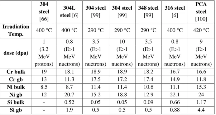
The complexity of the irradiation effects on stainless steel make it difficult to separate out the individual irradiation effects on stress corrosion cracking (SCC). Initially, chromium depletion at the grain boundary was considered a likely cause for IASCC, however, detailed studies have found that the lower chromium content at the grain boundary is not likely the controlling mechanism causing the increased cracking susceptibility [5,6]. In recent years, studies have shown a connection between the localization of deformation in irradiated stainless steel and IASCC [2,3,7–10]. While a connection between localized deformation and IASCC has been observed, the exact mechanism causing cracking remains unknown.

Localized deformation is a result of defects created by the irradiation severely hindering the motion of dislocations through the grains of the stainless steel. When a critical resolved shear stress is reached, the dislocations begin to slip through the defects created by the irradiation. As the dislocations pass through the irradiation damaged zone, defects are annihilated, creating a pathway with less resistance to slip for subsequent dislocations to pass through. As additional dislocations pass through the channel defects are progressively removed from the planes where slip has occurred. This forms what is termed dislocation channels, which consist of parallel slip planes where irradiation

(25)

3

defects have been cleared, creating a passage through which dislocation may pass with relatively low resistance. Dislocation channels are typically ~100 nm wide and space one to three microns apart.

One difficulty in understanding the role of localized deformation is determining an accurate way to analyze the amount of strain in the dislocation channel, and its effect on the grain boundary (amount of plastic/elastic strain it induces at the boundary). In this work, topographical measurements have been used to determine the height of the channel where it intersects the surface, and use this height measurement to approximate channel strain [11]. Height measurements can only be used as an approximation of total strain, as any strain in the surface plane is not measured. In plane strain has been studied in both unirradiated and irradiated metals using digital image correlation (DIC) [10,12], which refers to the comparison of two images of the sample surface at the same location, one prior to strain, one after plastic strain has been induced. Localized in-plane strain measurements are determined by measuring shifts in a pattern applied to the sample surface prior to strain. A random gold nano-particle speckle pattern was used in this work to allow for high resolution DIC to determine the in-plane displacement of the dislocation channels. By combining topographic measurements with DIC results, it was possible to measure displacement along all of the axes of the sample.

This thesis focuses on the interactions of dislocation channels with grain boundaries and the role of dislocation channeling on IASCC. Chapter 2 of this thesis describes relevant background information, in particular describing prior research that lead to this study. Chapter 3 describes the experimental procedures and the systems/techniques used in this study. Chapter 4 contains the results of the deformation

(26)

4

and cracking experiments. Chapter 5 is the discussion of the results presented in chapter 4, focusing on the relationship between the deformation measurements and cracking. Chapter 6 ends this thesis with the conclusions of this study.

(27)

5

Chapter 2

BACKGROUND

In this chapter, a review of published literature provides the background information relevant to the objectives and goals of this thesis. The first section describes the properties of the material of interest, austenitic stainless steel. The second section describes the deformation behavior of unirradiated polycrystalline materials such as stainless steel. This lays the foundation for understanding localized deformation that occurs in irradiated materials. The third section describes microstructure characteristics of importance to this study, namely grain orientation and grain boundary geometry. The fourth section discusses the effects of irradiation on austenitic steel. The fifth section describes the localized deformation processes that occurs in irradiated steel. The sixth section reviews irradiation assisted stress corrosion cracking (IASCC), the increase in cracking susceptibility that occurs due to irradiation effects in the steel. The seventh section discusses the current understanding of the relationship between localized deformation and IASCC. The final section states the objective of this work and the experimental approach used to accomplish the stated objective.

2.1 Properties of austenitic stainless steel

Steel is an iron alloy containing small amounts of carbon, generally less than 2 wt%. Steel may be separated in to three general phases: austenite, ferrite, and martensite.

(28)

6

Austenitic stainless steel is a form of steel containing chromium and nickel. The austenite phase is stabilized by nickel, carbon, nitrogen and manganese. Chromium decreases the stability of the austenite phase, but is added to increase corrosion resistance [13,14]. It is heavily used due to its strength, malleability and good corrosion resistance.

2.1.1 Physical and mechanical properties

While physical properties may vary depending on composition, generally austenitic stainless steels have a density of ~7.9 g/cm3 and are non-magnetic. It has a liquidus temperature of around 1400 °C and a low mean coefficient of expansion, ~1.9 × 10-5 °C-1 for temperatures between 20-1000 °C, which make it suitable to be used in high temperature conditions such as in nuclear power plants.

Typical yield strength and ultimate tensile strength for various commercial stainless steels is shown in Table 2.1. Mechanical properties of steel, such as yield strength, are dependent on the composition, grain size and level of cold work. The effect of grain size on yield strength can be characterized by the Hall-Petch relation [15],

0 1 2 y y k d    (2.1)

whereyis the measured yield stress, 0 is a friction stress, ky is a coefficient used to

characterize the transfer of slip through the grain boundaries and d is the grain diameter. Larger grain diameters result in softer steels. Austenitic stainless steels do not lose strength as rapidly at high temperatures as ferritic steels [16]. As depicted in the plot of yield strength vs. temperature of an austenitic steel in Figure 2.1, the yield strength of

(29)

7

austenitic stainless steel has a very shallow negative slope with increasing temperature between 100-600°C.

2.1.2 Phases

Steel is often composed of multiple phases, with combinations of austenite, ferrite and martensite. Unlike ferrite (BCC) and martensite (BCT), austenite has a face centered cubic (FCC) structure. The FCC structure is formed from three planes of close packed atoms, generally referred to as A, B and C, so as to form the repeating pattern ABCABC. The location of atoms relative to each other in these three planes is depicted in Figure 2.2.

As stated previously, different alloying elements stabilize different phases. This is depicted in a Schaeffler diagram, which relates percent ferrite to equivalent chromium and equivalent nickel values in the alloy. The equivalence equations relate other alloying elements in the steel to either a weighted chromium or nickel concentration. Various groups have created Schaeffler diagrams using different weighting factors and taking in to consideration different alloying elements [14,17,18], such as the one shown in Figure 2.3. Martensite may form in austenite during cold work. Equation (2.2) [19,20] is used to calculate the temperature at which 50 vol% martensite is formed after a true tensile strain of 30%: ( ) 413 13.7(% ) 9.5(% ) 8.1(% Mn) 18.5(% Mo) 9.2(%Si) 462(% C % N). d M C   Cr  Ni      (2.2)

Other phases that may form in austenitic steel include carbides, nitrides, and a σ-phase, which is generally an iron-chromium intermetallic that forms during prolonged heating in the temperature range of 650-870 ºC [14]. Carbon is much more soluble in

(30)

8

austenite at high temperatures. In some austenitic steels, carbon is only retained in the solution by rapid cooling, so that the carbon is trapped in solution, not having enough energy to form carbides, which would otherwise be more stable at the lower temperatures. If these steels are held at higher temperatures (450-850 ºC), carbides may precipitate and form, typically at the grain boundaries [13]. The σ-phase will always form after carbides have begun to precipitate. When the intermetallic phase forms, it can lower the Cr and the Mo content of the steel, which increases the carbon solubility and can lead to partial dissolution of carbides [20].

There are several types of carbides that may form. M23C6 commonly forms in

austenitic steels, where M represents Fe, Mo, Cr and Ni. MC may also form, with M representing Ti, Nb, or V. If Mo is present, M6C may form, from Fe, Mo and Cr. Carbon

content in austenitic steels is typically not high enough to form M7C3 (M representing Cr

and Fe). However for steels with high carbon contents, or in areas where C concentration is higher, M7C3 may form [20]. These carbides are typically undesired, as they are can

cause cracks to form at their interfaces and further cracking can result due to cracking propagation through the material [21].

M23C6 in austentic steels is typically composed of Cr and C, however Fe, Mo, and

Ni atoms may be substituted in place Cr atoms, and N and B atoms may substituted in for C atoms. Thermal history has a strong influence on the composition of the carbide. It forms an fcc crystal structure, and the lattice parameter is approximately three times that of austenite, though the lattice parameter is a function of the composition. M23C6 will

most likely precipitate at the grain boundaries, specifically at grain boundaries with high Σ values. After grain boundaries, the most likely locations for the carbide to precipitate

(31)

9

dislocations within the grain. Cold deformation can accelerate the carbide precipitation, specifically within the grains. M23C6 can cause intergranular corrosion and decreases the

ductility and toughness of the steel. It has been shown, however, to make grain boundary sliding more difficult when it is present at the boundary, thus improving creep ductility [20].

The MC carbide typically forms whenever Ti, Zr, Hf, V, Nb, or Ta are present in the austenitic steel. These elements are typically called stabilizing elements. While they lower the solubility of carbon in steel, they also lower the formation of M23C6 so that

there is less of a tendency for intergranular cracking. The MC carbide forms typically within the grain, on dislocations and stacking faults, though precipitation at the grain boundary can occur[20]. It is an fcc crystal structure and nitrogen can substitute in for the carbon to form a MN nitride.

M6C forms in steels containing Mo, and as most austenitic steels do not contain

high levels of Mo, M6C is typically not found, or only found in small amounts. When it

does form, it has an fcc crystal structure. M7C also does not typically occur in austenitic

steels, as the carbon content generally isn’t high enough. It requires a very high carbon:chromium ratio, higher than would be found in normal austenitic steel. It has a pseudo-hexagonal crystal structure. Table 2.2 summarizes the information for each of the four carbides previously discussed.

2.1.3 Corrosion

While stainless steel is generally considered to be corrosion resistant, it has been found to be susceptible to stress corrosion cracking (SCC) [13,22,23], as well as general

(32)

10

and localized (pitting/crevice) corrosion [24]. The good corrosion resistance of stainless steel largely comes from the passive oxide layer that the chromium forms over the metal surface. This compact, thin oxide layer significantly reduces any further corrosion.

When exposed to specific corrosive environments, and being under stress, usually from some combination of residual stress from the cold working of the material and an applied stress occurring during service, SCC has occurred in steel. Higher nickel compositions (>30 wt%) make the alloy more resistant to SCC, but do not completely mitigate the cracking. The heat treatments the steel has undergone will also affect the SCC susceptibility. Internal residual stresses may provide the stress necessary for SCC in certain environments. Heat treatments may relieve these stresses and therefore reduce SCC susceptibility, provided stress is not applied to the steel after the heat treatment. If carbides precipitate during the heat treatment (generally occurs between ~430 -870°C), however, cracking susceptibility will increase. A corrosive environment must be present for SCC to occur. In the case of stainless steel, SCC generally occurs in solutions that either contain chloride ions or are caustic. Dissolved oxygen, and high temperatures also will increase SCC susceptibility.

General corrosion is the term for the roughly uniform loss of material over the entire exposed surface. Due to the passive layer that readily forms over stainless steel, general corrosion is not typically a problem. However, if the steel does not have high enough levels of alloying elements which stabilize the passive film, in particular chromium, or is located in extreme environments such as acids and hot caustic solutions, general corrosion may occur.

(33)

11

In some cases, localized areas on the steel will corrode, rather than the entire surface. This typically results in pitting or crevice corrosion and is a result of imperfections in the oxide film or effects of the localized environment. Localized corrosion is generally enhanced by the presence of halogenides, such as chlorides, which can hamper the reformation of the protective oxide layer [25]. Chloride and sulfate ions in particular promote corrosion and cracking in stainless steel. Chlorides promote pitting and crevice corrosion, as well as increasing the rate of stress corrosion cracking. Chlorides effect sensitized steel in particular, though have been known to increase the corrosion of nonsensitized steels. Sulfates are more aggressive than chlorides in promoting IGSCC [26]. As little as 100 ppb sulfate ions can decrease the time to failure by a factor of three, due to increased IGSCC [27].

Generally, stainless steel suffers from intergranular stress corrosion cracking (IGSCC) in boiling water reactor (BWR) normal water chemistry (NWC) environments, though pitting does occur. Cases of cracking in stainless steel were observed as early as the 1950s in stainless steel fuel rods [28]. Table 2.3 outlines observations of different cases of cracking occurring of stainless steel in BWR environments. Studies of the corrosion of the steel components has been of interest due to economical, as well as safety concerns. The rate of cracking is a factor of the impurities in the water, as well as the oxygen content [26]. Figure 2.4 depicts the crack growth rate of two stainless steels with respect to water conductivity: the higher the conductivity (the higher the ion concentration), the more severe the cracking. Corrosion of steel in nuclear reactors will be discussed in more detail in a later section where irradiation assisted stress corrosion cracking is discussed.

(34)

12

2.2 Microstructure characteristics of polycrystalline materials

Grain boundaries, a result of the difference in orientation between the two adjacent grains, affect the mechanical properties of the material. In this section the grain orientations, or crystallographic texture, as well as the grain boundaries, where different crystal lattices meet between grains, will be discussed in context of effects on the properties of the polycrystalline material.

2.2.1 Grain orientation and crystallographic texture

Crystallographic texture refers to the distribution of grain orientations within a polycrystalline material. Grain orientation is related to mechanical properties, such as the resolved shear stress acting on slip systems as described by the Schmid factor. Texture may be examined locally by examining individual grain orientations, or by examining the general orientations within the material as a whole.

Orientation maps, such as the one shown in Figure 2.5, are one method for depicting individual grain orientations within a polycrystalline material. These maps show grain orientation, as well as spatial information about the location of the grain. The spatial information is particularly important when examining local phenomena, such as crack characterization at particular locations, as well as providing information not only about the grain orientation, but also the orientation of neighboring grains.

When examining the general orientation of all the grains in the material, it is common to simplify the analysis by examining only the orientation information of the grains, and not any of the spatial information, such as the location of the grain within the material. Pole figures are stereographic projections of the lattice orientations and are a

(35)

13

common method of presenting orientation data. Figure 2.6 demonstrates how a pole figure is created. A sphere is made to surround a unit cell of the lattice, and a stereographic projection is made of the points where lines normal to the lattice planes intersect the sphere.

2.2.2 Schmid and Taylor factors

A number of models have been created to describe macroscopic stress/strain by crystallographic properties, namely based on grain orientation [29–31]. Schmid and Taylor factors will be described in this section. The Schmid factor does not directly describe slip within a grain, however, it does examine the resolved shear stress acting on a single slip system, which is important when considering the critical resolved shear stress needed to initiate slip on that slip system. Taylor factor describes slip within a grain during straining of a polycrystalline material.

As stated previously, slip will not occur until a critical resolved shear stress, 𝜏𝑐, has been reached on the slip system. For uniaxial applied tensile stress, this may be calculated as

c cos cos

   , (2.3)

where 𝜎 is the applied tensile stress, 𝜆 is the angle between the slip direction and the tensile axis, and 𝜑 is the angle between the slip plane normal and the tensile axis. This is depicted graphically in Figure 2.7. Equation (2.3) may be shortened to

c m

   , (2.4)

(36)

14

mcos cos  (2.5)

For a slip system aligned to maximize shear stress from the applied tensile stress, the Schmid factor is at a maximum (m = 0.5). For a slip system oriented such that the slip direction is either parallel or perpendicular to the tensile axis, there is no shear stress acting on the system and the Schmid factor is minimized (m = 0). Grains may also be described by the Schmid factor of the slip system with the highest Schmid factor. Figure 2.8 shows the relationship between the orientation of the tensile axis and Schmid factor for a FCC crystal.

In Taylor’s plasticity analysis [30], it was assumed that all grains undergo the

same change in shape as the entire polycrystalline material. This assumption is depicted graphically in Figure 2.9. Taylor also assumed that all deformation occurred through crystallographic slip and the shear stress required to cause slip was the same for all slip systems. He concluded that the least work possible to impose the shape change in the grains would require that at least five (of the twelve in FCC) slip systems were active. For any given crystal orientation, Taylor selected the combination of five slip systems that resulted in the lowest sum of shear strains required to meet the overall shape change of the grain, assuming the other seven slip systems underwent zero shear strain.

When minimizing work performed in the slip systems, the incremental work/volume (dw) cause by slip in a given grain was defined as

i i

(37)

15

where τi is the shear stress required for slip to occur in slip system i, and γi is the shear

strain in that slip system. Given the assumption that shear stress required to cause slip is the same for all slip systems, τi is a constant and may be moved to the outside of the

summation. Using

x x

dw = d (2.7)

for the work/volume expressed in terms of external (applied to the macroscopic polycrystalline material) stress, σx, and strain, εx, along the tensile axis x. Equating the

work in the grains and the external work,

xd x d

    , (2.8)

Where dγ is the sum of dγi from Equation (2.6). The Taylor factor (M) is defined as

x x

Md / d   / . (2.9)

A high Taylor factor means that the grain had to undergo a lot of slip in order to match the overall shape change of the polycrystalline material, which means that a high Taylor factor grain will require more applied stress in order to undergo the necessary strain. For a FCC material, Taylor factor can range from 2.449 to 3.674, depending on crystal orientation, as described by Figure 2.10. Detailed descriptions of Taylors work can be found in more recent books describing mechanical behavior of materials by authors such as Hosford [32].

(38)

16

A grain boundary is defined as the surface between two crystal lattices, which are at different orientations from each other. Due to mismatch of the lattices and an imperfect union between the two adjacent lattices, more free volume exists in the grain boundary than a perfect lattice. Read and Shockley have shown that this is similar to a network of dislocations and that grain boundaries may be modeled as an array of dislocations [33]. The amount of free volume is dependent on the mismatch of the adjacent lattices.

In 1949, a special subclass of grain boundaries were classified by Kronberg and Wilson [34]. These boundaries, called coincident site lattice (CSL) boundaries, are special due to the similarity in adjacent lattices which causes the two grains to match well at the boundary. To better understand the structure of CSL boundaries, the lattices of the two adjacent grains are visualized as overlapping, as shown in Figure 2.11, which depicts a Σ5 boundary. CSL boundaries are denoted by a Σ value, which is the reciprocal of the ratio of the number of coincident sites to all lattice sites (e.g. so in the Σ5 boundary type, one in five lattice sites are in coincidence). CSL boundaries may also be described by rotation and an axis of rotation. These are listed for CSL boundaries Σ < 30 in Table 2.4. A number of studies have shown that the energy associated with grain boundaries decreases sharply when the boundary is a CSL when compared to RHABs of similar orientations [35–37]. This is especially true for Σ3 (twin) boundaries. An example of this is shown in Figure 2.12, where grain boundary energy for a number of boundaries is compared. Reported in these results is the relative grain boundary energy, with the boundary at 129° serving as the reference energy.

(39)

17

In general, a grain boundary is just an interface. As could be expected of any type of interface, the cohesion strength may be affected by defects at the interface. In the case of grain boundaries, the cohesion strength may be weakened by mechanical defects (non-bonded regions, such as those caused by missing atoms from dislocation or voids) and chemical segregation of impurities to the interface (could affect the spacing of atoms in the lattice or create additional, weaker interfaces, that lead to stress concentrations at the boundary interface) [38]. Temperature and emission of dislocations are also stated to affect cohesion strength, as well as the angle of the grain boundary tilt [39].

While a stress may be applied uniformly to a polycrystalline sample, the stress will not be uniformly distributed throughout the sample, due largely to the anisotropy of the deformation properties of grains, and the random crystal orientations in most polycrystalline material. In particular, stress tends to be higher at grain boundaries, likely due to the effect of the crystallographic orientations of neighboring grains. An example from a finite element model done by Kamaya et al. [40] is shown in Figure 2.13. In particular, stress may be particularly high at triple junctions, the point where three grains meet [40–42].

2.3 Deformation behavior in unirradiated face centered cubic (FCC) polycrystalline material

Under high levels of stress, crystalline materials will deform through the movement of dislocations along slip systems. On the macroscopic level, deformation begins at the yield stress of the material, which will elongate along the direction of the applied stress and reduce in the dimensions normal to the applied stress. On the microscopic level, strain is more complex in polycrystalline materials. Depending on the

(40)

18

orientation of the grains, slip may occur in certain grains before the applied stress has reached the macroscopic yield stress.

2.3.1 Dislocations and slip systems

In general, metals deform through the slip of dislocations through the crystal lattice. Dislocations are generally defined as edge dislocations and screw dislocations. Edge dislocations act as an extra half plane of atoms within the lattice and produce slip in the direction the dislocation moves. The magnitude and direction of the distortion in the lattice caused by the dislocation is equal to the Burgers vector (b) of the dislocation. For edge dislocations, the Burgers vector is perpendicular to the dislocation. In the case of screw dislocations, the Burgers vector is parallel to the dislocation line.

In an FCC crystal structure, edge dislocations tend to move along the {111} planes and in the <110> directions, for a total of 12 slip systems. Dislocations will not move along the slip plane until a critical resolved shear stress has been reached. This was discussed more in the section on Schmid factor. Obstacles within the grain, and the grain boundaries themselves, act to impede the movement of dislocations. When encountering an obstacle that the dislocation is unable to move through, edge dislocations may move perpendicular to the slip plane through a process called climb. Climb is a diffusion process, where interstitials or vacancies diffuse to the dislocation, causing the movement perpendicular to the slip plane. In the case of interstitials, the dislocation half plane is lengthened, whereas vacancies cause it to move in the opposite direction, shortening the half plane. As it is a diffusion process, climb is more likely to occur at high temperatures. Interactions between dislocations and grain boundaries will be discussed in more detail later in this section.

(41)

19

2.3.2 Stacking fault energy and partial dislocations

A stacking fault results when a plane of atoms is added or removed from the repeating ABCABC pattern of the FCC close packed planes. The stacking fault is considered intrinsic when a plane is removed, resulting in ABCA|C, with the stacking fault represented by the |. An extrinsic stacking fault results from the addition of a plane within the pattern, such as ABCACBC, where an additional C plane is added, represented by the C. There is an energy associated with the change in order of the close packed lanes, called the stacking fault energy (SFE), which is an intrinsic property of an alloy.

SFE is related to the composition of an alloy. There are several empirical correlations relating SFE and composition, though they are not consistent with each other. In general, they follow the form

2

(mJ/ m ) _Const _i _i(wt .%), i

SFE X 



X C

(2.10)

where the constants (X) were determined empirically, and the concentrations (C) of the alloying elements are known. Table 2.5 depicts three sets of constants from different empirically derived fits of composition to SFE. As a result of the high degree of variation in SFE models, when accurate values are required, they must be derived experimentally. Equation (2.10) and the constants found in Table 2.5 are better suited for relative approximations [7].

Stacking faults form when a perfect dislocation dissociates into two partials (the stacking fault exists between the two partials). In order to minimize the energy required to move the dislocation, it is often divided into two partial dislocations, which each act as

(42)

20

half of the full dislocation. A perfect dislocation with a Burgers vector of 1 2[101]



b

may divide into 1 6[1 12]



b and 1

6[112]



b partial dislocations, as shown in Figure 2.14.

These two partial dislocaitons tend to be divided by a number of atomic planes, rather than occurring over a single plane as shown in Figure 2.14. The two partials repel each other, however, the existence of the stacking fault between them also increases the overall energy of the lattice, and so the SFE pushes them together in order to minimize the increase in energy caused by the stacking fault. In materials with a low SFE, the partials will be separated by a larger distance than in a material with a high SFE. Due to the large spacing between partials, it is difficult for the dislocation to cross slip between slip planes, as the partials must recombine prior to the cross slip. As a result, low SFE materials generally undergo planar slip. Austenitic stainless steels generally have low SFEs.

2.3.3 Interactions between dislocations and grain boundaries

As stated previously, and depicted in Equation (2.1), grain size affects the strength of a material. Specifically, smaller grains result in higher yield stresses. This is a result of grain boundaries acting as obstacles to dislocation slip. When a dislocation encounters a grain boundary, there are several different forms of interactions that may occur, which may be generally divided into discontinuous slip and slip accommodation. Discontinuous slip refers to the case where a dislocation encounters a grain boundary and is pinned with no further slip occurring. Slip accommodation may refer to direct slip transmission across the grain boundary, cross slip into a different slip system within the same grain, nucleation of new dislocations, or absorption into the grain boundary. These cases of dislocation interactions with the grain boundary are depicted in Figure 2.15.

(43)

21

When a dislocation cannot be accommodated at the grain boundary, it will remain in the lattice near the grain boundary. As the crystal is strained further, additional dislocations will move through the lattice towards the grain boundary and form a dislocation pile-up. Dislocations of like signs will repel each other, however, the applied stress on the crystal will push the dislocation towards one another, as they are unable to pass through or into the grain boundary. This creates an area of high str