Fault Diagnosis Using Kernel Principal Component Analysis for Hot Strip Mill

(1)

University of Wollongong

Research Online

Faculty of Engineering and Information

Sciences - Papers: Part B

Faculty of Engineering and Information

Sciences

2017

Fault Diagnosis Using Kernel Principal Component Analysis for

Hot Strip Mill

Fei Zhang

University of Wollongong, [email protected]

Shengyue Zong

University of Science And Technology Beijing

Zhi Ling

University of Science And Technology Beijing

Follow this and additional works at:

https://ro.uow.edu.au/eispapers1

Part of the

Engineering Commons

, and the

Science and Technology Studies Commons

Recommended Citation

Zhang, Fei; Zong, Shengyue; and Ling, Zhi, "Fault Diagnosis Using Kernel Principal Component Analysis for

Hot Strip Mill" (2017). Faculty of Engineering and Information Sciences - Papers: Part B. 1498.

https://ro.uow.edu.au/eispapers1/1498

(2)

Fault Diagnosis Using Kernel Principal Component Analysis for Hot Strip Mill

Abstract

In the field of hot rolling process monitoring, the activation of non-linear dynamic behaviour may render

the procedure of fault diagnosis more difficult. Principal component analysis (PCA) is known as a popular

method for diagnosis but as it is basically a linear method, it may pass over some useful non-linear

features of the system behaviour. One possible extension of PCA is kernel PCA (KPCA), owing to the use

of non-linear kernel functions that allow introduction of non-linear dependences between variables. The

objective of this study is to address the problem of fault diagnosis (in terms of non-linear activation) in

hot rolling automation system using a KPCA-based method. The detection is achieved by comparing the

subspaces between the reference and a current state of the system through the concept of subspace

angle. It is shown in this work that the exploitation of the measurements in the form of KPCA can

effectively improve the detection results.

Disciplines

Engineering | Science and Technology Studies

Publication Details

F. Zhang, S. Zong & Z. Ling, "Fault Diagnosis Using Kernel Principal Component Analysis for Hot Strip Mill,"

Journal of Engineering, vol. 2017, (9) pp. 527-535, 2017.

(3)

Fault diagnosis using kernel principal component analysis for hot strip mill

Fei Zhang

1,2

, Shengyue Zong

1

, Zhi Ling

1 1

Institute of Engineering Technology, University of Science and Technology Beijing, Beijing 100083, People

’

s Republic of

China

2

School of Electrical, Computer & Telecommunications Engineering, University of Wollongong, Wollongong, NSW 2522,

Australia

E-mail: [email protected]

Published inThe Journal of Engineering; Received on 16th May 2017; Accepted on 11th August 2017

Abstract:In theﬁeld of hot rolling process monitoring, the activation of non-linear dynamic behaviour may render the procedure of fault diagnosis more difﬁcult. Principal component analysis (PCA) is known as a popular method for diagnosis but as it is basically a linear method, it may pass over some useful non-linear features of the system behaviour. One possible extension of PCA is kernel PCA (KPCA), owing to the use of non-linear kernel functions that allow introduction of non-linear dependences between variables. The objective of this study is to address the problem of fault diagnosis (in terms of non-linear activation) in hot rolling automation system using a KPCA-based method. The detection is achieved by comparing the subspaces between the reference and a current state of the system through the concept of subspace angle. It is shown in this work that the exploitation of the measurements in the form of KPCA can effectively improve the detection results.

1 Introduction

A significant process in the areas of manufacturing and processing of metals is the tandem rolling of hot metal strip. In the case of steel, almost one-half of thefinished product made in the world is in the form of sheet and strip that originally is produced in a hot strip rolling process. While this unquestionably reflects a fundamental drive of the industry for higher efficiency production, more specific factors include operation rationalisation moves such as the syn-chronisation with continuous casting plant, and a series of equip-ment refurbishequip-ments aimed at higher product quality [1].

Hot strip rolling is a kind of high-production and high-efﬁciency industrial process. Its purpose is to process cast steel slabs into steel strip with a wide range of thickness. Because of its huge size and large investment a hot strip mill need to have a lifetime of sev-eral decades. The mill must be capable of meeting the market demands for a wide range of steel grades, in particular, high strength and advanced high strength steels with good cold formability and with superior strip properties.

The primary function of the hot strip mill (HSM) is to reheat semi-finished steel slabs of steel nearly to their melting point, then roll them thinner and longer through some successive rolling mill stands driven by motors, andfinally coiling up the lengthened steel sheet for transport to the next process. The slabs, of up to 35 t weight, are typically 250 mm thick and 10 m long, and the rolled strips are typically 2 mm thick and 1250 m long. The reheat furnace ensures that the slab is at a suitable temperature to start hot rolling, which is∼1200°C. The next unit, the roughing mill (RM), is responsible for major reductions in slab thickness (e.g. a reduction from 200 to 30 mm). The transfer table carries the slab, now called a transfer bar, from the RM to thefinishing mill (FM). The transfer bar is typically 40–90 m long and 0.5–1.5 m wide. A relatively recent development in hot strip mill design, the coilbox, is sometimes used to wrap the transfer bar into a coil in order to obtain a more uniform temperature profile along the strip. The transfer bar is then peeled and fed into the FM, which pro-gressively squeeze the steel to make it thinner. As the steel becomes thinner, it also of course becomes longer, and starts moving faster. Because the single piece of steel will be a whole range of different thicknesses along its length as each section of it passes through a different stand, different parts of the same piece of steel are

travelling at different speeds. Dimensions of hot and thin strip, especially the width, are sensitive to tension variations. The tension variations are inevitable in tandem mills, because the roll rotation speeds cannot be regulated with sufﬁcient precision. In order to add a degree of freedom that prevents abrupt tension changes, and to serve as a sensitive indicator of tension variations, loopers are used. A looper is a metal cylinder supported by an arm free to move around a pivot. Keeping the strip above the pass line, it stores the extra amount of strip that is necessary for strip tension regulation. The strip emerging from the FM is typically much longer than the runout table; so, the coiling starts before the tail end leaves the FM. This requires very close control of the speeds at which each individual stand rolls; and the entire process is con-trolled by computer. By the time it reaches the end of the mill, the steel is travelling at about 40 miles per hour. Afterwards it is cooled down intensively by water sprays from coolant headers along the runout table and then winded up in a coiler, which is essentially a rotating mandrel. During this part of the process, piece temperatures are important and should be, typically, 870°C after the last rolling stand and 600°C at the coiler [2]. At the same time, a series of quality control measures, such as automatic thickness control (AGC), automatic width control, automatic shape control, and auto-matic temperature control, are implemented to guarantee the super-ior quality of the products.

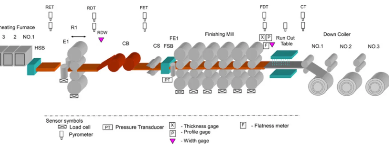
The outline of a typical 1700 mm HSM is illustrated in Fig.1, where R1 is the No. 1 stand of RM, HSB and FSB is the high-pressure descaling box and ﬁnishing descaling box, respectively, E1 and FE1 are the roughing edger mill and ﬁnishing edger mill, respectively, CB and CS are the coil box and crop shear, res-pectively, RET and RDT represent the RM enter and delivery tem-perature, respectively, FET and FDT represent the FM enter and delivery temperature, respectively, and CT represents cooling temperature.

Due to the demanding dimensional quality requirements and multitude of operating objectives, the FM has in time become a complex unit equipped with a high level of automation [3]. The surface quality, internal defects, shape, thickness, width and microstructure of the hot-rolled strip directly affect the quality of downstream processing products. Throughout the HSM automation system, there are 55 process variables affecting the 3 surface quality, 40 process variables affecting the internal defects, 36

(4)

process variables affecting the three coupled variables of the strip shape, plate thickness, plate width, and up to 108 process vari-ables affecting the microstructure and properties of materials [4]. These process variables include temperature, roll force, displace-ment, thickness, width, velocity, pressure, tension, torque, current parameters and so on. These process variables are coupled to each other, for example, the change of roll gap will affect the strip exit thickness, and then exit thickness changes will affect the forward slip, at the same time, the factors affecting the forward slip also include reduction, the friction coefﬁcient between the roller and the rolled piece and so on. Besides the mutual coupling characteristics, the rolling process variables also have the character-istics of non-linearity, uncertainty, large scale, multi scale and so on. Therefore, the rolling mill system is a very typical non-linear system, and there is a strong non-linear relationship between the process variables.

The complexity of rolling technology and the characteristics of high temperature, high pressure and high speed in hot rolling process determine the relatively high failure rate of automation system, and even a tiny fault in production process may cause sig-niﬁcant economic losses. In order to guarantee the quality of the products, and keep the rolling process in a continuous and reliable operation, the engineers and operators need real-time monitoring of the running conditions of the whole rolling process, especially the abnormal conditions that may affect the quality of products and safety of personnel and equipment.

The increasing pressure of competition and the tighter market are forcing the plant users to seek the optimum utilisation of their facil-ities, improved product quality and an extended product mix. All these presuppose a high availability of the plants and the avoidance of unforeseen failures. Moreover, the maintenance costs have to be reduced to a minimum in order to continue to be competitive. For a long time, due to the inability to predict the occurrence of faults, people have to take two measures: Theﬁrst is maintenance when the equipment failure, but which will lead to a large economic loss, high maintenance costs, and even casualties. The second is a regular maintenance of equipment, which has a certain planning and preventive, but a lot of blindness, may easily lead to ‘over repair’or‘under repair.’The technology of fault diagnosis is devel-oped with the historical evolution of equipment technology and the scientiﬁc development of maintenance activities, and makes the equipment maintenance history into the stage of condition based maintenance.

The prompt detection and precise diagnosis of faults become a main requirement for any enterprise for safe, optimal and proﬁtable operation. For that reason, the problem of fault diagnosis and diagno-sis for industrial processes has received considerable attention during the last two decades. Although of the non-linear characteristics of most of the industrial processes, the majority of the fault diagnosis

methods are of linear nature, e.g. principal component analysis (PCA). PCA is the most widely used data-driven technique for process monitoring since it can effectively deal with high-dimensional, noisy and highly correlated data by projecting the data onto a lower-dimensional subspace which contains most of the variance of the original data [5]. However, PCA sometimes shows quite a degraded performance when the process exhibits strong nonlinear correlations between its variables [6], and most of the existing non-linear PCA approaches are based on neural network, which has to solve a nonlinear optimisation problem[7]. Among the non-linear PCA techniques, KPCA developed by Schölkopf has been attracted because it does not involve non-linear optimisation [8], it is as simple as in linear PCA, and it need not specify the number of principal components (PCs) prior to modelling compared to other non-linear methods [9,10]. The core idea of kernel PCA (KPCA) is to ﬁrst map the data space into a feature space using a non-linear mapping and then compute the PCs in the feature space. It should also be noted that KPCA only requires the solution of an eigenvalue problem, and, since it can incorporate dif-ferent kernel functions, KPCA can handle a wide range of non-linearities. The main advantage of the KPCA method over referred non-linear PCA approaches is that no non-linear optimisation should be involved [7]. Leeet al.[11] used this method for non-linear process monitoring. Hiden et al. [12] suggested non-linear PCA using genetic programming. Shaoet al.[13] proposed a non-linear PCA based upon an input-training neural network. Cheng et al.

[14] used adaptive KPCA to monitor small disturbances of non-linear processes. Zhang [15] integrated KPCA and kernel independent component analysis for, respectively, monitoring the Gaussian part and non-Gaussian part of a process. Further, support vector machine is used to classify the fault types. Zhanget al.[16] used kernel partial least squares for non-linear process monitoring.

Although a lot of approaches have been used in the fault diagnosis of hot rolling process [17–23], but KPCA has not been found. This paper focuses on the development and application of KPCA techni-ques to address these concerns speciﬁcally within the steel industry. The motivation for the application of empirical-based methodolo-gies lies in the fact that monitoring and fault diagnosis can be carried out through process representations (models) which do not require the expert development of phenomenological models. KPCA is capable of efﬁciently modelling the non-linear relation-ships that exist between sensor measurements and quality variables. In this research, we use KPCA approach for hot rolling fault diagno-sis, and through the analysis of the test result, it is proved that the KPCA method is more effective than the PCA method.

This paper is organised as follows. Section 2 explains KPCA and its properties. In Section 3, the KPCA-based fault diagnosis to a HSM is presented and discussed. Finally, Section 4 provides con-cluding remarks.

Fig. 1 Typical hot strip mill layout

This is an open access article published by the IET under the Creative Commons Attribution License (http://creativecommons.org/licenses/by/3.0/)

J Eng, 2017, Vol. 2017, Iss. 9, pp. 527_–535 doi: 10.1049/joe.2017.0190

(5)

2 KPCA-based process monitoring

2.1 Algorithm of KPCA

As a simple linear transformation technique, PCA compresses high-dimensional data into low-dimensional with minimum loss of data information. When the algorithm is carried out in the feature space, KPCA is obtained. KPCA is a type of kernel-based learning machine. The key idea of KPCA is both intuitive and generic. The basic idea of KPCA is to map the input dataxinto a feature space F first via a non-linear mapping Φ, and then perform a linear PCA in_F. However, it is difficult to do so directly because the dimensionhof the feature spaceFcan be arbitrarily large or even infinite. In implementation, the implicit feature vector inF does not need to be computed explicitly, while it is just done by computing the inner product of two vectors in _F with a kernel function [24].

Given an initial data matrix,X, representingnobservations ofm

variables as X=(x1,x2, . . .,xn)= x₁₁ x₁₂ · · · x₁_n x₂₁ x₂₂ · · · x₂_n ... ... .. . ... x_m₁ x_m₂ · · · x_mn ⎛ ⎜ ⎜ ⎜ ⎝ ⎞ ⎟ ⎟ ⎟ ⎠ (1) with xi= x∗i− 1/n n i=1x∗i 1/n−1 x∗i− 1/n n i=1x∗i 2 (2)

where xi(i=1, 2, . . .,n) is then observations (column vectors) normalised from the n training samples x∗i(i=1, 2, . . .,n) of the input space. By the non-linear mapping Φ, the measured inputs are extended into the hyper-dimensional feature space as follows:

F:x[RmF(x)[Fh (3)

The mapping ofxiis simply noted asΦ(xi) =Φi. The sample

covari-ance in the feature space can be constructed by

C=1 n n i=1 FiF T i (4)

where non-zero eigenvalues of covariance matrixCare positive. A PCvis then computed by solving the eigenvalue problem

lv=Cv (5)

whereλdenotes eigenvalue andvdenotes eigenvector of the covari-ance matrix. HereCvcan be represented as

Cv=1

n

n i=1

kFi,vlFi (6) wherekx,yldenotes the dot product betweenxandy. This implies that all solutions v with λ≠0 must lie in the span of

F1,F2, . . .,Fn. Hence (5) is equivalent to

lkFi,vl=kFi,Cvl, i=1, 2, . . .,n (7) For anyλ≠0, there exists coefﬁcientsa_i(i=1, 2, . . .,n), such that

v= n

i=1

aiFi (8)

Then (9) can be deduced from (7) and (8)

ln i=1 aikFk,Fil= 1 n n i=1 aikFi n j=1 FjlkFj,Fil, k=1, 2, . . .,n (9) To obtain the coefﬁcientsa_i(i=1, 2, . . .,n), a kernel matrixKof dimension n×n is deﬁned, and its elements are determined by virtue of kernel tricks

Kij=FTiFj=kFi,Fjl=k(xi,xj) (10) wherek(_xi,_xj) is the calculation of the inner product of two vectors inFwith a kernel function.

A number of kernel functions exist. According to Mercer’s theorem of functional analysis, there exists a mapping into a space where a kernel function acts as a dot product if a kernel func-tion is a continuous kernel of a positive integral operator. The requirement of the kernel function is to therefore satisfy Mercer’s theorem [25]. The representative kernel functions are as follows:

Polynomial kernel

k(_x,_y)=kx,yld (11)

Sigmoid kernel

k(x,y)=tanhb₀kx,yl+b₁ (12)

Radial basis kernel

k(_x,_y)=exp −x−y

2

c

(13)

whered,β0,β1andcare speciﬁed a priori by user. The polynomial

kernel and radial basis kernel always satisfy Mercer’s theorem while the sigmoid kernel satisﬁes it only for some values of β0

and β1 [26]. The speciﬁc choice of a kernel function implicitly

determines the mappingφand the feature spaceF. If one has a non-linear information of process, it could be used to select the kernel function among kernels in KPCA. Before applying KPCA, mean centring and variance scaling in high-dimensional space should be performed.

Then (9) can be simpliﬁed to

nlKa=K2a (14)

where a=a₁,a₂, . . .,a_n T identiﬁes the eigenvector _v after normalisation.

Notice that before applying KPCA, we have to perform mean-centring procedure since the gram matrix used for the above eigen-value problem is not mean-centred. The centred gram matrix_K¯can be easily obtained by ¯ K=K−EK−KE+EKE (15) with E=1 n 1 · · · 1 ... ... ... 1 · · · 1 ⎛ ⎜ ⎝ ⎞ ⎟ ⎠[Rn×n (16) From (14)–(16), theﬁnal eigenvalue problem in KPCA approach is to solve

nla=_K¯a (17)

The coefﬁcient α should be normalised to satisfy a 2=1/nl, which corresponds to the normality constraint _v 2=1 of eigenvector.

(6)

Cumulative percent variance (CPV) is utilised to determine numberdof PC, i.e. CPV(d)= d i=1li n i=1li .CL (18) where CL is the control limit.

Then the dimension reduction can be achieved by retaining the

ﬁrst d eigenvectors. After constructing the PCs in the feature space F, the score vector of the kth observation in the training data set can be obtained by projecting the centred value F¯(x) onto the eigenvectors vk in F of the new sample x, where

k=1, 2, . . .,d, such that t_k=kv_k,Fl¯ = n i=1 ak,ikF¯i,Fl¯ = n i=1 ak,iK¯(xi,x) (19) where the mapping ofxis simply noted asΦ(x) =Φ. Using (18), we

ﬁnally obtain a score vectort= t1,t2, . . .,td

T

forx.

For the special case in whichF(_x)=_x, KPCA is equivalent to linear PCA. From this viewpoint, KPCA can be regarded as a gen-eralised version of linear PCA.

2.2 Online monitoring procedure

Generally, the fault diagnosis based on PCA uses two statistics, Hotelling’s T2 and SPE. Hotelling’s T2 represents Mahalanobis distance of an observation on the PCA model subspace. On the other hand, SPE represents the Euclidean distance from the model space. Such statistics in the feature space can be obtained using energy decomposition [27, 28]. The observations obtained from a signiﬁcantly nonlinear process are highly non-Gaussian due to the non-linearity. Hence, the non-linear mapping to the higher-dimensional feature space is formulated such that the train-ing samples conform to a Gaussian distribution after the nonlinear mapping. Then, the distribution of the mapped training data can be estimated by a normal probability density inF. The corresponding energy, represented by the negative logarithm of the probability, is given by

V(x)=FTC¯−1F (20)

where the mapping of x is simply noted as Φ(x)=Φ, C¯

denotes the regularised covariance matrix, which is calculated as follows:

¯

C=vLvT+l⊥I−vvT (21)

whereΛis a diagonal matrix of eigenvalues associated with the retained PCs,λ⊥is a constant value which replaces all zero or near-zero eigenvalues in_Cfor regularisation, and_Iis an identity matrix. Substituting the regularised covariance matrix into (20), we can de-compose the energy into two parts, one is a Mahalanobis distance in the KPCA space and the other is a Euclidean distance from the model subspace as follows:

V(x)= d k=1 l−1 k kvk,Fl2+l⊥ F 2− d k=1 kvk,Fl2 =tTL−1t+l⊥−1k(x,x)−tTt =T2+l−_⊥1SPE (22)

where the mapping ofxis simply noted asΦ(x) =Φ.

Therefore, two monitoring statistics for new observation xnew,

T_new2 andSPEnewcan be written as follows:

T_new2 =tTnewLtnew (23)

SPE_new=k(xnew,xnew)−t T

newtnew (24)

The conﬁdence limit forT2can be determined byF-distribution

T_lim2 =d(n−1)

n−d Fd,n−d,a (25)

whereFd,n−d,αdenotes aF-distribution with the degree of freedom

dandn−dwith the level of signiﬁcance 100(1−α)%.

For SPE, we used the same rule as linear PCA to obtain 100(1−α)% control limit as follows:

SPE_lim=u₁ ca 2u₂h2 0 u1 +1+u2h0(h0−1) u2 1 1 h₀ ui= D j=d+1 li j, h0=1− 2u₁u₃ 3u2 2 ⎧ ⎪ ⎪ ⎪ ⎪ ⎪ ⎪ ⎪ ⎨ ⎪ ⎪ ⎪ ⎪ ⎪ ⎪ ⎪ ⎩ (26)

whereDdenotes the effective dimension of feature space discussed below.

Because the dimension of feature space is arbitrarily high, the control limit of SPE may be unrealistically large. Hence the effective dimension of feature spaceDis empirically determined as the smallest number of the ordered eigenvalues whose cumula-tive sum is above 99% of the sum of all eigenvalues.

3 KPCA-based fault diagnosis to a HSM

If the fault diagnosis of HSM is to be carried out, the data acquisi-tion system of the monitoring signal should be set up atﬁrst, and different acquisition techniques and methods should be adopted according to different signal types.

3.1 Signal selection

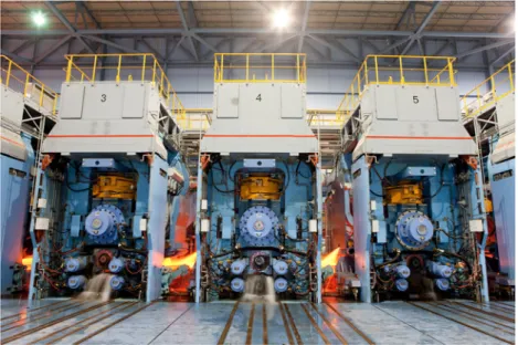
There are hundreds of kinds of control and monitoring signals for a single stand of HSM, so it is impossible for us to choose all the signals. AGC is the most important mechanism for dynamic thickness control in conventional rolling mills. Since the AGC system is responsible for maintaining the dynamic performance of the predicted quality of thickness, it is designed to suppress the disturbances during the rolling process such as hardness and temperature fluctuation of the strip. The extremely sophisticated algorithms are developed to fulfil the task of dynamic thickness control, however, the philosophy and the principles for tuning AGC control gains become very complicated and difficult to the operators in the case of improving the quality for specific product and process [29]. The rolling stands of HSM are shown in Fig.2, from which we can find the hydraulic actuators, known as roll force cylinders, are installed above the top backup roll chocks. Hydraulic actuator is the main equipment to implement AGC.

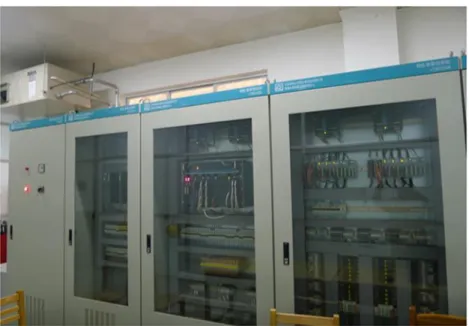
Considering the main factors affecting the gauge, we select process variables including roll gap, roll force, roll bending force and delivery thickness. Here in order to verify the effectiveness of the algorithm, we only select the 19 AGC-related signals or mea-sured variables which are illustrated in Table1. As shown in Fig.3, all signals connected to the control cabinets are received by pro-grammable automation controllers.

(7)

3.2 Data acquisition

Measurements on all process variables, including those up to the FM, were recorded for each coil rolled over a one week period of production. For this study, the manufacture of a single grade of steel coil on a six-stand FM was considered.

Theﬁrst stage was to carry out data pre-screening to eliminate or correct data anomalies such as missing data and outliers. The data was then divided into two sub-sets, _XM and _XV _XM comprised data on the next-of-batch coils, whileXV included the

ﬁrst-of-the-batch coils. Previous statistical studies have shown that the variation in the quality parameters was greater for the

first-of-batch coils than for later coils in the batch. In terms of out-of-specification product, the variation is small; however, in eco-nomic terms, the benefits of tighter control limits can yield signifi -cant savings. Since data setXMconsisted of 612 coils rolled with the correct roll gap settings that corresponded to products that met customers’ specifications, it was used to generate a nominal process representation. Data setXV, with 224first-of-batch coils, formed the test data on which the proposed techniques were evaluated.

Measured data is collected by ibaPDA (Process Data Acquisition) system from programmable automation controllers. The ibaPDA system is a PC-based acquisition and analysis system for measured values. It is made up of distributed hardware com-ponents for signal acquisition, connections via optical ﬁbres and other media, such as PROFIBUS-DP, boards for standard PCs or notebooks, as well as online recording software and ofﬂine analysis software. Besides recording, the online software also offers a user-friendly visualisation function for an unlimited number of channels with ongoing line diagram presentation, similar to a recorder.

The ibaPDA system features a modular design with hetero-geneously structured signal acquisition lines. ibaPDA is capable of processing a very large number of channels in a uniform and

synchronous manner. This makes the ibaPDA system particularly suitable for distributed and multiple systems. The measured data gathered is saved in ﬁles on the hard disk of the online PC or on specialﬁle servers. Fig.4shows the system topology with one-server and multiple clients. The one-server is a basic process in ibaPDA which handles the data acquisition and storage, and it can run independently from and without a client.

3.3 Fault diagnosis

The substantial growth in the use of automated in-process sensing technologies creates great opportunities for manufacturers to detect abnormal manufacturing processes and identify the root causes quickly. It is critical to locate and distinguish two types of faults: process faults and sensor faults. Sensor is a window to understand the process state, and its effectiveness is the prerequisite and basis for the implementation of process control, process optimisation and other fault diagnosis. Dependable sensor data are vital in complex systems, which rely on a suite of sensors for control as well as condition monitoring. With any unanticipated deviations in sensor values, the challenge is to determine if the anomalies are the result of one or moreﬂawed sensors or if it is indicative of a potentially more serious system-level fault. This paper mainly studies the sensor fault.

Sensor fault diagnosis is also known as instrument fault diag-nosis, instrument validation, sensor calibration and so on. A sensor (instrument) usually includes a sensing device, a transducer, a signal processing unit, and a communication interface. Any part of the above may be faulty, and then the deviation from the sensor output signal and the actual value of the variable (nominal value) exceeds the allowable range. Sensor faults are classiﬁed into four types: bias, drift, precision degradation, and complete failure [30].

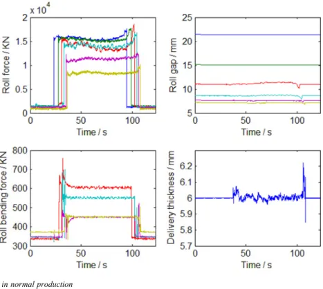
Signal curves of HSM in normal production are illustrated in Fig. 5, where the curves of the roll gap, roll force and roll bending force refer to the curves of the six FM stands, and the delivery thickness only refers to the FM delivery thickness. These signals play important roles in hot rolling process. Sensor faults of the roll gap, roll force, roll bending force and delivery thickness will seriously deteriorate theﬁnal quality of hot rolled production if not detected. Various sensor faults may occur in the rolling process. Through analysis, different types of sensor faults are found out from the historical data. In order to demonstrate the fault recognition effects of KPCA, four different faults

Fig. 2 FM stands in rolling process

Table 1 Summary of AGC-related signals

No Signal name Number of signals

1 roll gap of the six FM stands 6

2 roll force of the six FM stands 6

3 roll bending force of the six FM stands 6

(8)

corresponding to the above mentioned four types, respectively, are selected for validation.

As shown in Fig.6, the faults during rolling process include: (1) a step bias of roll force sensor of F2,

(2) a drift change of roll gap sensor of F4,

(3) a precision degradation of roll bending force sensor of F3, (4) a complete failure of delivery thickness sensor,

where Firepresents the ith stand of FM. All faults are actual faults which have a serious impact on the quality of the products during the production process, which comes from the data collected by the ibaPDA system. And these faults have been conﬁrmed by the

ﬁeld engineer.

In all cases, the sampling interval is 0.01 s, and the rolling pro-cesses are displayed for 16 s, with the faults starting at the 8th second. Then 1600 data points are collected to use for KPCA mod-elling in the 16 s production period.

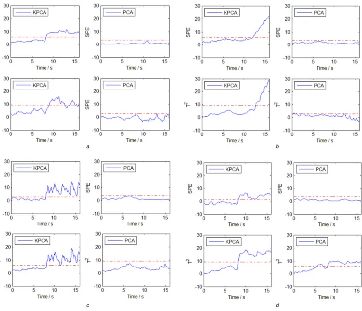
The SPE and T2charts for KPCA and PCA monitoring of the rolling process are shown in Figs.7a–d. It is evident from these charts that KPCA shows relatively correct fault diagnosis in comparison to PCA, whether theT2 or SPE statistics. The above study demonstrates that compared to PCA, KPCA can effectively capture the non-linear relationship among process variables and its application to hot rolling process monitoring shows better performance than PCA. These fault identiﬁcation results prove the validity of the KPCA approach. However, this method should not be overestimated, because sometimes fault cannot be

Fig. 3 Control cabinets of HSM automation system

Fig. 4 Server–client topology of the ibaPDA system

(9)

recognised clearly or even misclassiﬁed. Further studies are still necessary.

4 Conclusions

In this paper, a fault diagnosis method based on KPCA was formu-lated for supervising hot rolling processes. Thanks to its capability to process data in a nonlinear way, KPCA presents some advantages with respect to other methods like PCA which are basically linear procedures. The sensitivity of KPCA regarding the detection of

the onset of non-linear dynamic behaviour has been illustrated using measured data from a HSM with non-linear characteristics. The method provides powerful tool for ensuring consistent high-quality products at the same time helping the operators in their de-cision making. The importance of manufacturing zero-defect coils, in the face of increasing global competition in the steel processing industries cannot be underestimated.

The main drawback of KPCA (with respect to PCA) is the com-putation time. Since the number of measured signals is often much smaller than the number of time samples, PCA may be performed

Fig. 5 Signal curves of HSM in normal production

(10)

economically using singular value decomposition of the observa-tion matrix and the size of the PC matrix does not exceed the number of measurements. Regarding KPCA, data is at ﬁrst mapped to a high-dimensional feature space whose dimension equals the number of time samples. For this reason, the eigen-problem to solve in the feature space may be costly if the dimension is too high. It requires a limitation of the length of the signals to avoid a too demanding computation.

5 Acknowledgments

This work was partially supported by Innovation Method Fund of China (no. 2016IM010300) and National Natural Science Funds of China (no. 51404021).

6 References

[1] Takagi K., Hotta H., Watanuki M.: ‘Kawasaki Steel Technical Report’, 1991, (24), pp. 64–74

[2] Reeve P.J., MacAlister A.F., Bilkhu T.S.:‘Control, automation and the hot rolling of steel’,Philos. Trans. R. Soc. A, Math. Phys. Eng. Sci., 1999,357, (1756), pp. 1549–1571

[3] Yildiz S.K., Forbes J.F., Huang B.,ET AL.:‘Dynamic modelling and simulation of a hot stripﬁnishing mill’,Appl. Math. Model., 2009, 33, (7), pp. 3208–3225

[4] Peng K., Zhou D., Li N.:‘Quality-related monitoring and control in hot strip mill process’, Control Eng. Chin., 2011, 18, (4), pp. 650–654

[5] Cho J.H., Lee J.M., Choi S.W.,ET AL.:‘Fault identiﬁcation for process monitoring using kernel principal component analysis’,Chem. Eng. Sci., 2005,60, (1), pp. 279–288

[6] Dong D., McAvoy T.J.:‘Nonlinear principal component analysis-based on principal curves and neural networks’, Comput. Chem. Eng., 1996,20, (1), pp. 65–78

[7] Ge Z., Yang C., Song Z.:‘Improved kernel PCA-based monitoring approach for nonlinear processes’,Chem. Eng. Sci., 2009,64, (9), pp. 2245–2255

[8] Schölkopf B., Mika S., Burges C.J.C.,ET AL.:‘Input space versus feature space in kernel-based methods’, IEEE Trans. Neural Networks, 1999,10, (5), pp. 1000–1016

[9] Zhang Y., Qin S.J.:‘Improved nonlinear fault detection technique and statistical analysis’,AIChE J., 2008,54, (12), pp. 3207–3220 [10] Zhang Y., Li S., Teng Y.:‘Dynamic processes monitoring using

recursive kernel principal component analysis’, Chem. Eng. Sci., 2012,72, pp. 78–86

[11] Lee J.M., Yoo C.K., Choi S.W.,ET AL.:‘Nonlinear process monitoring using kernel principal component analysis’,Chem. Eng. Sci., 2004, 59, (1), pp. 223–234

Fig. 7 Fault diagnosis results for sensor faults

(a)Bias of roll force sensor of F2,(b)Drift change of roll gap sensor of F4,(c)Precision degradation of roll bending force sensor of F3,(d)Complete failure of delivery thickness sensor

(11)

[12] Hiden H.G., willis M.J., Tham M.T.,ET AL.: ‘Non-linear principal components analysis using genetic programming’, Comput. Chem. Eng., 1999,23, (3), pp. 413–425

[13] Shao R., Jia F., Martin E.B.,ET AL.:‘Wavelets and non-linear principal components analysis for process monitoring’,Control Eng. Pract., 1999,7, (7), pp. 865–879

[14] Cheng C.Y., Hsu C.C., Chen M.C.: ‘Adaptive kernel principal component analysis (KPCA) for monitoring small disturbances of nonlinear processes’, Ind. Eng. Chem. Res., 2010, 49, (5), pp. 2254–2262

[15] Zhang Y.:‘Enhanced statistical analysis of nonlinear processes using KPCA, KICA and SVM’, Chem. Eng. Sci., 2009, 64, (5), pp. 801–811

[16] Zhang Y., Fan Y., Du W.:‘Nonlinear process monitoring using regression and reconstruction method’, IEEE Trans. Autom. Sci. Eng., 2016,13, (3), pp. 1343–1354

[17] Gu D.W., Poon F.W.:‘A robust fault-detection approach with appli-cation in a rolling-mill process’,IEEE Trans. Control Syst. Technol., 2003,11, (3), pp. 408–414

[18] Theilliol D., Mahfouf M., Sauter D.,ET AL.:‘Actuator fault detection, isolation method and state estimator design for hot rolling mill monitoring’,IFAC Proc. Volumes, 2006,39, (13), pp. 843–848 [19] Dong M., Liu C.:‘Design of fault diagnosis observer for HAGC

system on strip rolling mill’,J. Iron Steel Res. Int., 2006,13, (4), pp. 27–31

[20] Yildiz S.K., Huang B., Forbes J.F.:‘Dynamics and variance control of hot mill loopers’,Control Eng. Pract., 2008,16, (1), pp. 89–100

[21] Rother A.: ‘Approach for improved signal-based fault diagnosis of hot rolling mills’, PhD Thesis, Universität Duisburg-Essen, 2016 [22] Bai Q., Jin B., Gao Y.,ET AL.:‘An online fault pre-warning system of the rolling mill screw-down device based on virtual instrument’,Sens. Transducers, 2014,168, (4), pp. 1–7

[23] Jiang L., Fu X., Cui J., et al:‘Fault detection of rolling element bearing based on principal component analysis’. 2012 24th Chinese Control and Decision Conf. (CCDC), Taiyuan, China, May 2012, pp. 2944–2948

[24] Cui P., Li J., Wang G.: ‘Improved kernel principal component analysis for fault detection’, Expert Syst. Appl., 2008, 34, (2), pp. 1210–1219

[25] Christianini N., Taylor J.S.: ‘An introduction to support vector machines and other kernel-based learning methods’ (Cambridge University Press, Cambridge, England, UK, 2000)

[26] Haykin S.: ‘Neural networks—a comprehensive foundation’ (Prentice-Hall Inc., Upper Saddle River, NJ, USA, 2007, 3rd edn.) [27] Cremers D., Kohlberger T., Schnörr C.:‘Shape statistics in kernel

space for variational image segmentation’,Pattern Recognit., 2003, 36, (9), pp. 1929–1943

[28] Choi S.W., Lee C., Lee J.M.,ET AL.:‘Fault detection and identiﬁcation of nonlinear processes based on kernel PCA’,Chemometr. Intell. Lab. Syst., 2005,75, (1), pp. 55–67

[29] Zhang F., Zhang Y., Chen H.: ‘Automatic gauge control of plate rolling mill’, Int. J. Control Autom., 2016, 9, (2), pp. 143–156

[30] Kusiak A., Song Z.: ‘Sensor fault detection in power plants’,

Research Online Research Online

Faculty of Engineering and Information Sciences - Papers: Part B

Faculty of Engineering and Information Sciences

works at: https://ro.uow.edu.au/eispapers1

Engineering Commons

, and the Science and Technology Studies Commons

https://ro.uow.edu.au/eispapers1/1498

ch Online: https://ro.uow.edu.au/eispapers1/1498