1
Firing the Wrong Workers:
Financing Constraints and Labor Misallocation
Andrea Caggese
Pompeu Fabra University, CREI, BGSE
Vicente Cuñat
London School of Economics
Daniel Metzger
Stockholm School of Economics*
October 2017
Abstract
Firms consider wages, current and expected productivity as well as firing and hiring costs when firing a worker. Financing constraints distort this intertemporal trade-off, leading firms to sub-optimally fire short-tenured workers with high future expected productivity. We provide empirical evidence of this distortion using matched employer-employee data from the Swedish population between 2000 and 2010. We propose a new empirical strategy that uses credit ratings to identify financing constraints and uses exchange rates and trade data to identify demand shocks. Our empirical results identify an important new misallocation effect of financial frictions that operates within firms across different types of workers.
JEL classification: G32, J21, J24, J31 Keywords:
Labor misallocation, Firing decisions, Financing constraints
* Corresponding Author: Vicente Cuñat, [email protected], LSE, Department of Finance, Houghton Street, WC2A 2AE London, UK. Andrea Caggese: [email protected], Daniel Metzger: [email protected]. We would like to thank Xavier Giroud, Harald Hau, Markus Schmid, Christoph Schneider, Toni Withed and an anonymous referee as well as seminar participants at the NBER Summer Institute 2016, the Labor and Finance Conference in Capri, AFA 2017, and 27th Mitsui Finance Symposium: Labor and Corporate Finance for their helpful comments and suggestions. We also thank Christoph Albert, Marta Alonso-Sanz and Virginia Minni, who provided excellent research assistance. The authors acknowledge the financial support of Resercaixa and AXA.
2 1. Introduction
The effect of financing frictions on the investment decisions of firms is a
long-standing question in economics. Asymmetric information, transaction costs or agency
problems may limit the ability of firms to pledge future expected profits to raise funding,
making them financially constrained and unable to finance profitable investment
opportunities. The existing empirical literature has mostly focused on how the lack of
financing can reduce the size of total physical investment (Hubbard, 1998). More
generally, however, financing constraints distort any intertemporal decision that has cash
flow implications by favoring projects that generate more cash or save costs in the short
term (see, for example, Eisfeldt and Rampini, 2006). This type of trade-off is also relevant
for many labor-related decisions that involve paying an upfront cost to improve the future
expected productivity of the workforce, such as searching, screening, training, and firing.
The objective of the paper is to study how financing constraints affect the firing
decisions of firms. In particular, we argue that financing constraints influence the types of
workers who are fired across firms and have an important distortionary effect on the
optimal allocation of employees, even when they have little effect on the total employment
level. When deciding on which workers to fire, firms consider several factors, such as the
current and future expected productivity and wages of a worker as well as firing and hiring
costs. A firm may, for instance, be indifferent between firing a recently hired promising
worker with low firing costs or a longer-tenured worker with low productivity growth but
higher firing costs. Although all firms face similar trade-offs, financing constraints distort
this decision, as constrained firms place more weight on current cash flows than on future
3
To illustrate these ideas and to guide our empirical analysis, we develop a stylized
partial equilibrium model of a firm that makes hiring and firing decisions regarding
heterogeneous workers. Financial frictions make credit-constrained firms discount future
cash flows more severely than unconstrained firms.In the model, the productivity of
workers varies during their tenures, so firms must keep replacing them to maximize
productivity, even in the presence of firing costs. Moreover, recently hired workers have
the potential to become more productive in the future, and therefore, their value for the
firm includes an option component. Another key feature of the model is that wages are
rigid and do not fully adjust to compensate for fluctuations in the productivity of workers.
Finally, firing costs increase with workers’ tenure in the firm.
In equilibrium, relative to normal times, a temporary negative demand shock makes it
optimal for financially unconstrained firms to fire more long-tenured workers than
short-tenured ones because the value of recent hires depends on future growth prospects and is
less affected by temporary drops in their profitability. In this context, financial frictions
affect not only the overall level of firm employment but also the optimal mix of
short-tenured and long-short-tenured workers. More financially constrained firms have a higher
opportunity cost of money and discount the option value of short-tenured workers more
heavily, placing a larger weight on short-term returns. Moreover, long-tenured workers are
less likely to be fired in constrained firms that have a higher opportunity cost of paying
their firing costs. Finally, the higher firing hazard of short-tenured workers in constrained
firms implies that a smaller fraction of them become long-tenured workers. As a
consequence, the model implies the following four testable hypotheses. First, all else
equal, the more financially constrained a firm is, the more likely it will be to fire a
4
more financially constrained a firm, the shorter the tenure profile of its labor force. Third,
in the event of a temporary exogenous shock that requires a reduction in employment, a
financially unconstrained firm will fire more long-tenured workers than it would in normal
times. Fourth, in the event of the same shock, a more financially constrained firm will fire
relatively more short-tenured workers than a less constrained firm. These distortions
operate through a labor demand channel and imply that financing constraints induce firms
to fire workers with high productivity growth prospects, generating labor misallocation in
equilibrium.
To understand the empirical relevance of the distortions, we analyze the effects of
financing constraints on (i) the average firing policies of firms across tenures, (ii) the
tenure profile of the labor force, (iii) the firing policies after an exogenous negative shock,
and (iv) the types of workers fired. We test the predictions of the model using matched
employer-employee data from the whole active population of Sweden over two decades:
between 1990 and 2010. We match worker information with employer information, for
which we have extensive balance sheet and credit score data. The exceptional quantity and
quality of information available in this data set makes it ideal for our objective.
We measure financing constraints using well-established ratings of the population of
Swedish firms. To match our empirical analysis with our theoretical setup, we focus on
those firms with good ratings. Among these firms, different ratings imply heterogeneous
access to credit and different interest rates. However, the firms in our sample are not
financially distressed. We identify financing constraints in three different ways. First, we
use three discrete rating categories, provided by the main rating company in Sweden, that
5
equilibrium correlations between firing and financing constraints. Second, we use a
regression discontinuity design (RDD) that uses the thresholds (on a continuous risk
measure) that determine credit ratings. Small differences in an underlying continuous
default probability measure lead to discrete changes in a public rating that have important
consequences for the perception of the creditworthiness of the firm. Our design exploits
this discrete change in perceived creditworthiness by comparing firms that are arbitrarily
close to a rating boundary but are on the different side of the threshold. Finally, the
structure of the data allows us to compare long- and short-tenured workers within a firm in
a given year. The specification absorbs any time-varying characteristics that affect both
types of workers within a firm.
To identify exogenous changes in firing hazards, we use shocks to the exchange rate
of a firm-specific basket of currencies. We construct this basket using the country
composition of a firm’s exports at the beginning of the sample period.
Our analysis concentrates on comparing the firing of short-tenured workers – who, on
average, have steeper productivity profiles and lower firing costs – with that of
long-tenured workers. We first show that, on average, financially constrained firms employ
more short-tenured workers than unconstrained firms. Second, after suffering an exchange
rate appreciation shock, both constrained and unconstrained firms are more likely to fire
workers. Importantly, however, we find significant differences in the types of workers
fired across firms. On the one hand, the shock causes more firing of long-tenured workers
in unconstrained firms, relative to normal times. The model predicts such behavior as a
positive reallocation effect of temporary negative shocks, during which unconstrained
6
workers with more productivity growth potential. We perform additional robustness checks
using a measure of expected productivity growth at the worker level that confirms this
interpretation. On the other hand, constrained firms that suffer a negative shock fire more
short-tenured than long-tenured workers, in comparison to financially unconstrained firms.
Taken together, these results imply that financial frictions not only reduce the job stability
of short-tenured workers but also generate an inefficient allocation of workers across firms
and over time.
Quantitatively, we find that small exogenous changes in financing frictions generate
potentially large distortions in the form of excessive firings of short-tenured workers.
When we identify differences in financial frictions using the boundary between the two
highest credit rating categories, we find that an increase in the cost of external financing of
0.15 percentage points implies that following an exogenous appreciation shock, the
likelihood of being fired for short-tenured workers increases by approximately 10%
relative to the average firing probability.
Finally, constructing empirical measures of the average productivity and expected
productivity growth of workers, we provide direct evidence that these firing decisions of
constrained firms are inefficient because they involve workers with relatively higher
expected productivity growth than the workers fired by unconstrained firms.
Overall, the results are consistent with our analytical predictions and highlight an
important – but relatively unexplored – form of misallocation: Financially constrained
firms fire short-tenured workers with high skills and positive productivity growth
7
We believe that the results of the paper can be easily extrapolated to other labor
market settings. In any dual labor market, with fixed-term and permanent workers, or in a
labor market where severance payments increase with tenure, the studied effects are likely
to be relevant and very strong. Moreover, even in the absence of regulatory frictions or
severance pay, the interaction between financing constraints and worker productivity
growing with tenure would generate the same results. Therefore, the main effects identified
in the paper are generally applicable to most labor markets. Given that both financing
constraints and labor frictions are, in relative terms, low in Sweden, one can interpret the
results as a lower bound for the effect in other developed countries.
2. Related Literature
This paper is related to the recent empirical literature that studies the effects of
financial frictions and financial shocks on the employment decisions of firms (see Pagano
and Pica, 2012). Recent papers such as Chodorow-Reich (2014) for the U.S. and Bentolila,
Jansen, Jiménez, and Ruano (2013) for Spain study the causal link from financial shocks to
fluctuations in net employment levels, focusing on the quasi-natural experiment of the
financial crisis.1 Our paper differs from these studies because it focuses on exogenous
profitability shocks at the firm level rather than on aggregate financial shocks, and on their
differential effect on constrained versus unconstrained firms. More importantly, it focuses
on the effects on the type of workers fired and not the level of employment.
Our theoretical model and its predictions are based on the key insight that by
increasing the opportunity cost of capital in the short term, financial frictions reduce the
incentive to select projects with short-run costs and long-run gains that would be attractive
8
in the absence of financing constraints. Other authors that use the same insights are
Eisfeldt and Rampini (2006), who study the effect of financial frictions on the trade-off
between the decisions to buy new or used capital. Similarly, Caggese and Cuñat (2008)
study the effects of financial frictions on the trade-off between hiring with fixed-term or
permanent contracts. The latter can be a useful instrument to attract more productive
workers but comes with larger expected termination costs.2
It is worth putting the paper in perspective with another stream of the literature that
concentrates on the effects of financial distress on labor supply (e.g., Brown et al., 2016
and Baghai et al., 2016). In particular, Baghai et al. (2016) use similar data of Swedish
workers to measure workers’ voluntary departures in the three years prior to bankruptcy. In
contrast, we measure the effects of financing constraints on labor demand and focus on
relatively healthy firms to avoid capturing the influence of financial distress.3
3. Analytical Framework
In this section, we analyze a stylized model of a firm with heterogeneous workers and
provide a set of testable predictions on the relation between financial frictions and firing
decisions. The model focuses on the implications of the following three key features. First,
2More generally, the theoretical model of this paper is related to the recent literature on financial frictions and the
misallocation of resources across firms (see, for example, Buera, Kaboski and Shin, 2011; Caggese, and Cuñat, 2013; Midrigan and Xu, 2014) and on the literature on financial frictions, the dynamics of hiring and firing, and employment fluctuations (among others, see Wasmer and Weil, 2004; Monacelli, Quadrini, and Trigari, 2011; Petrosky-Nadeau, 2014; Petrosky-Nadeau and Wasmer, 2015; Caggese and Perez, 2016).
3
This contrasts with Baghai et al. (2016), who look at firms that have filed for bankruptcy. Instead, we focus on healthy firms with a credit rating between 1 and 3 (see Section 4.1. for details). The yearly propensity for initiating a bankruptcy process for firms with a rating between 1 and 3 is 0.68% (compared with 7.09% for lower rated firms). Applying our additional filters reduces this likelihood to 0.35% in our sample.
9
wages are rigid and do not fully adjust to compensate for fluctuations in the productivity of
workers. Second, recently hired workers have more upside potential than long-tenured
workers. Third, firing costs increase with workers’ tenure in the firm. For simplicity, the
model considers the trade-off between firing short-tenured workers vs. long-tenured
workers regardless of their age. However, the assumption that short-tenured workers have
steeper productivity profiles than long-tenured ones implies that the model can also be
interpreted as predicting how financing constraints affect the firings of younger versus
older workers.
3.1. The model
Each worker produces an output equal to , where A is firm-specific productivity, is worker specific productivity, is the number of workers, and ∈ 0,1 is a
parameter capturing the elasticity of total firm output to total labor input . A newly hired
short-tenured worker has an initial productivity equal to , drawn from a uniform
distribution [ , . Every short-tenured worker has a probability of becoming long-tenured.
Conditional on becoming long-tenured, the worker draws a new productivity value,
, from a uniform distribution [ , , where 1 is the parameter that measures the ability of workers to become more productive as they accumulate more experience in the
firm. This simple structure implies that while on average, workers become more
productive with tenure, some of them may become less productive.
Firms can fire short-tenured workers without cost and long-tenured workers by paying
a fixed firing cost, F>0, and they can hire new short-tenured workers by paying a fixed
10
observed only after the wage is decided and that the wage cannot be changed afterwards,
and we derive the optimal decisions in the steady state, with constant interest rate r and
firm-level productivity A. It follows that the optimal wage is constant both over time and
across workers, and the optimal number of workers is also constant over time, i.e., .
Therefore, to simplify the analysis, we fix the wage , and the associated division of
surplus between firm and workers, at an arbitrary value that can be considered a
reduced-form representation of wage bargaining. At the end of this section, we relax this
assumption and allow the wage to partly adjust to reflect fluctuations in worker
productivity. Note that Sweden is one of the countries with the highest wage compression
in the world, so the assumption that wages do not fully react to worker productivity is
particularly relevant in our empirical setting.4
The timing of the interaction between the firm and the workers is as follows: at the
beginning of each period, a worker exogenously leaves a firm with probability , and the
firm decides whether to fire workers who stay. Among continuing workers, a fraction of
the short-tenured workers become long-tenured, while some new short-tenured workers are
hired. Then, all workers produce and are paid a wage 0.
Value of long-tenured workers
We define as the value of a long-tenured worker who is employed in the firm
until she quits, as a function of her productivity:
4In particular, wage compression guarantees that more productive workers are also more profitable for the firm. In
countries where wages react more to individual worker productivity, the impact of worker productivity on firm profits should be smaller.
11 1 1
(1)
where is the market interest rate, and is a wedge that incorporates financial
considerations; i.e., it is higher for more financially constrained firms. This wedge is a
reduced-form measure of different types of financial frictions, such as higher opportunity
costs of money caused by credit rationing, higher costs of borrowing, and higher
bankruptcy probability. This definition of financial constraints can potentially identify both
differences in restrictions to credit and interest rate differentials. Since our model and
testable hypotheses are consistent with both types of frictions, we abstract from these
considerations throughout the paper and consistently use the term financing constraints to
refer to these rating differences. Since productivity is constant over time, , it
follows that
1 (2)
A short-tenured worker with current productivity who has not been fired in the current
period has the following value:
1 1
1
1 1
(3)
which can be simplified as follows:
1
1
1 1
(4)
where the expected value conditional on becoming long-tenured, , is equal to
1 2
1 2
12
where is the minimum productivity of continuing long-tenured workers, and it will be
determined in the next section.
3.2. Employment-level decisions
The optimal employment level is determined by the following free entry condition:
0 (6)
Since is linear in , and workers are uniformly distributed across the values
of , it follows that the expected value of a new short-tenured worker is
1 2
1
2 (7)
where is the minimum productivity of a short-tenured worker to avoid being fired.
Using equation Error!Referencesourcenotfound. to substitute in Error!Reference
sourcenotfound., it is possible to derive the optimal number of workers n, which is
inversely related to financing frictions.
Proposition 1: is negatively related to .
A higher value of financing frictions λ both increases the opportunity cost of hiring new workers, v 1 r λ , and reduces V . For a formal proof, see Appendix 2. 3.3 Firing decisions in the steady state
Given the free entry condition, short-tenured workers who have overly low
productivity and have a negative value for the firm will be fired and replaced by a new
worker such that the minimum productivity satisfies
13
and any short-tenured worker with productivity is fired and replaced with a new
worker. A firm will replace a long-tenured worker if her value is negative and larger in
absolute value than firing costs such that the minimum productivity satisfies
(9)
The relation between and is affected by two counteracting forces. On the
one hand, the value of a short-tenured worker benefits from the option value of becoming
very productive in the future. From equations Error!Referencesourcenotfound., Error!
Referencesourcenotfound. and Error!Referencesourcenotfound., it immediately
follows that . In other words, at the productivity level , a
short-tenured worker is more valuable than a long-short-tenured one. The difference,
, increases with the value of the parameter , which measures the growth opportunities of short-tenured workers. If this difference is larger than firing costs , then
, and the firm is more likely to fire a long-tenured than a short-tenured worker
conditional on a given productivity level , even though the long-tenured workers are
costlier to fire.
On the other hand, a higher value of financing frictions reduces the value of
long-tenured workers relative to the opportunity cost of firing, F, and reduces , meaning that a more financially constrained firm will less frequently fire long-tenured workers.
Moreover, it reduces the net present value of the future productivity of short-tenured
workers, thereby reducing their option value and increasing . Therefore, both effects
14
Proposition 2: A more financially constrained firm is likely to fire short-tenured workers more frequently than a less financially constrained firm with the same profitability, A, and
the same quality of workers.
See Appendix 2 for a formal proof. Taken together, the above analysis shows that
constrained firms are likely to fire short-tenured workers more frequently than
unconstrained firms because financial frictions reduce the option value of these workers.
Moreover, the higher firing hazard of short-tenured workers implies that a smaller fraction
of them become long-tenured workers, thus increasing the share of short-tenured workers.
Conversely, long-tenured workers become more difficult to fire, which increases the
relative share of long-tenured workers. If firing costs are relatively low, as is the case of
Sweden, the first effect is likely to prevail; therefore, we also predict that a more
financially constrained firm will, in equilibrium, have a younger workforce.
3.4. Firing decisions after a shock
In this section, we assume that a temporary shock hits a firm at the beginning of a
period, thereby reducing A. This reduced-form shock can be interpreted as any productivity
or demand shock that reduces the revenues of the firm. For simplicity, we assume that this
shock lasts only one period. The above equations imply that the value of workers decreases
such that and increase and the firm fires both some short-tenured and
long-tenured workers that period. Assuming that firing costs are relatively low and the growth
prospects of young workers are relatively high, such that , it follows that the
value of short-tenured workers for a firm relies heavily on their productivity growth
15
productivity shock affects them less than long-term workers, and increases relatively
less than .
Proposition 3: Following a temporary drop in A, a financially unconstrained firm reduces employment by firing relatively more long-tenured workers than during normal times.
Proposition 3 implies that a temporary negative shock has a positive reallocation effect
in which less productive workers—especially among those with longer tenures and fewer
growth options—are fired across the tenure spectrum.
Furthermore, we can study the effect of financing frictions on the mix of short-tenured
and long-tenured workers who are fired. From equation Error!Referencesourcenot
found., it follows that the more a firm is financially constrained, the more the value of its
short-tenured workers is driven by current profitability rather than by the
option value of becoming more productive in the future, . Therefore, a
temporary drop in A will have a much larger negative effect on the value of short-tenured
workers for more financially constrained firms.
Proposition 4: Following a temporary drop in A, the more constrained a firm is, the more it fires short-tenured workers rather than long-tenured workers.
See Appendix 2 for a formal proof. It is important to note that financial frictions
determine these predictions, as well as the steady-state predictions, by reducing the
expected value of short-tenured workers (option value channel), increasing the opportunity
cost of laying off more senior workers (firing cost channel), or both channels
simultaneously. When firms are financially constrained, both channels increase the firing
16
are not too high, the option value channel is responsible for a higher equilibrium level of
short-term workers in constrained firms and for the broader firing effect of financially
unconstrained firms.
3.5. Empirical predictions and empirical strategy
The model described above implies the following testable predictions:
Hypothesis 1: The more financially constrained a firm is, the more likely it fires a
short-tenured worker, and the less likely it fires a long-short-tenured worker.
Hypothesis 2: The more financially constrained a firm is, the younger the tenure profile of
its labor force is.
Moreover, after an exogenous shock that requires a reduction in employment:
Hypothesis 3: A financially unconstrained firm reduces employment by firing relatively
more long-tenured workers than it would during normal times.
Hypothesis 4: A more financially constrained firml fires workers with shorter tenures.
It is important to note that predictions 1, 3 and 4 relate to firm-level decisions that are
conditional on the intensity of the financial frictions the firms face. As such, we expect
them to hold both when we compare firms with different intensities of financial frictions
and when we examine a single firm over different periods of time. However, prediction 2
refers to the differential flows in and out of each tenure category as well as their long-run
effects on the equilibrium tenure composition of the labor force. Therefore, we expect it to
hold when we compare persistent differences in financial frictions across firms but not
17
3.6. Firing and misallocation
Hypotheses 1 and 4 imply that more financially constrained firms inefficiently fire
workers with high growth prospects who would be retained by less financially constrained
ones. However, it is plausible that with other frictions that are not included in the model,
financing constraints could induce firms to make better employment decisions. It is
therefore useful to directly test the misallocation effects in financially constrained firms.
To empirically test this effect, we relax in the model the assumption of complete wage
compression and assume that workers are paid a wage 0, where 0 1
indicates the sensitivity of wages to labor productivity, and w is the fixed component. The
per-period profit that the firm receives from the worker becomes 1 , but it does not otherwise affect the optimality conditions of the model or the four previous
hypotheses. This assumption implies that more productive workers are paid more, but they
are also more profitable for the firm. Importantly, assuming that is greater than zero
allows us to identify, in the empirical section, both different productivity levels across
workers and their expected productivity growth using worker-level wage estimation
models. Therefore, we are able to directly verify the misallocation consequences of the
firing decisions of firms.
4. Data and Descriptive Statistics
This section describes the data set, and Section 5 describes the empirical strategy. A
detailed list of all the variables used in the analysis and how they are constructed is
18
4.1. Firm data
We test our hypotheses using matched employer-employee data of the universe of
Swedish firms available for the 1998-2010 period from the Swedish Companies
Registration Office (Bolagsverket), processed by the private data vendor PAR/Bisnode.
The data include balance sheets and income statements of all Swedish limited liability
companies (Aktiebolaget or AB).
We obtain rating information from UC AB, a rating agency owned by the largest four
banks in Sweden. It provides yearly, automated credit reports on all enterprises registered
in Sweden. Each report provides a discrete rating, commercially called a “credit score”.
Credit scores range from 1 (least constrained) to 5 (most constrained). These discrete
ratings are based on a continuous measure, “Risk Forecast”, of the annual probability of
default of the firm. Discrete thresholds of the continuous measure determine the 5 discrete
ratings.5 The average (median) rating throughout the whole population of firms is 1.97 (2),
suggesting that the firms in our sample are relatively unconstrained on average. The
sample of credit ratings as well as its underlying continuous default probability are
available for the 2001-2011 period.
International trade data are provided by Statistics Sweden and contain value
information by trade type (import/export), product (8-digit classification), and country for
each organization between 2000 and 2011. In terms of volume, the largest export markets
are Germany (10.2%), the USA (9.4%), Norway (9.0%), Great Britain (7.7%), Denmark
(6.0%), and Finland (5.3%). This diverse distribution of export markets is favorable for our
5
In the original UC AB data, 1 corresponds to “most constrained” and 5 to “least constrained”. We have reversed the order for our empirical analysis such that a higher number indicates higher financing constraints throughout the paper. The thresholds on the risk score are 0.245%, 0.745%, 3.045%, and 8.045% and are determined by UC AB.
19
purpose as they are located in different currency zones. We use these data to construct
empirical measures of firm-specific exchange rate movements. We follow Park et al.
(2010) and construct a weighted exchange rate, Shock Index, with respect to a basket of
currencies to which companies are exposed. There is some independent variation across
currencies, so different combinations of trading partners may imply that appreciations and
depreciations of the firm-specific baskets coexist in a given year. Note that even though the
export-based weights are kept constant throughout the sample, the Shock Index varies at a
firm-year level.
To include a firm in our sample, we impose the following additional requirements: i)
the firm employs at least 10 workers, ii) the firm appears for at least 5 consecutive years in
our sample, and iii) the yearly workforce growth is restricted to be within -50% and +50%.
Our final firm sample consists of 97,607 firm-year observations of 13,852 unique
firms. On average, we have approximately 9,000 firms per year. The distribution of
firm-years over our sample period of 11 firm-years between 2001 and 2011 is relatively balanced
over time with a minimum of 6.45% of all observations in 2001 and a maximum of
10.75% in 2007. The average age of firms is approximately 13 years. The mean (median)
employment is 102 (27) workers. The average annual growth rate of companies’ labor
force is 1.0%. A fraction of 34% of the workforce has been with the firms for less than
three years on average.
4.2. Worker data
Our basic sample is the “longitudinal integration database for health insurance and
labor market studies” (LISA) provided by Statistics Sweden (SCB). The database holds
20
registered in Sweden as of December 31 for each year. The data set contains employment
information such as employment status, the identity of the employer, and wages.
Although our firm sample contains data only from 2001 onwards, we make full use of
the whole sample period of LISA as it allows us to calculate the tenure of each worker
more accurately and run our auxiliary wage regressions more efficiently. Applying the firm
data requirements to the worker data results in a sample of approximately 6.9 million
person-year observations. The average (median) worker is 39 (38) years old and male
(66%) and has been with the firm for 3.5 years on average. Approximately 6.2% of all
workers are fired every year. We consider a worker as fired if i) she moves to a new firm /
no firm in the next year and ii) claims unemployment benefits in the current or in the next
year. The firing rates vary substantially by tenure. Approximately 10.3% of short-tenured
workers (0-2 years with the firm) but only approximately 2.8% of long-tenured workers
are fired every year.
5. Empirical Strategy
The main objective of the paper is to understand the firing policies of financially
constrained and unconstrained companies in good and bad times across types of workers.
In this section, we provide details about how we proxy for each of these measures as well
as the specifications used in the paper. Jointly, they determine the identification strategy of
the paper.
5.1. Measuring financing constraints
We use firm ratings as a measure of financing constraints. We focus on firms with
21
potentially subject to financial distress.6 While distressed firms are clearly financially
constrained, they also have characteristics that may make them undesirable for our
analysis. In particular, they may have a very short time horizon in their investment
decisions and strong incentives for risk-shifting through going concern. Therefore, their
incentives to fire or restructure the workforce may be very different from those of regular
firms outlined in our model.
Firm ratings directly measure the likelihood of default of a company; thus, they are a
good proxy for the availability and cost of credit for a firm. It is therefore useful to run
regressions that use ratings directly as a measure of financing constraints. Since they are
determined simultaneously with firm productivity, investment opportunities and current
policies, they must be interpreted as equilibrium relations between employment policies
and financing constraints. Hence, our first set of regressions for each specification uses the
first three discrete ratings of UC AB as a measure of financing constraints, with and
without including firm fixed effects.
However, it is also useful to run regressions in which we estimate the causal effect of
an exogenous change in financing constraints. To do so, we use two further identification
strategies: a regression discontinuity design (RDD) and a within-firm-year estimator.
The structure of our data (worker-year panel) allows us to make use of a
within-firm-year estimator. We saturate the model with firm-within-firm-year dummies and measure financing
constraints using the discrete credit rating variable. This specification absorbs any common
additive variation across worker types that is firm-year-specific. We therefore measure the
6
While the yearly likelihood of initiating a bankruptcy process is 0.68% for firms with a credit rating between 1 and 3, this likelihood increases to 7.09% for firms rated 4 or 5.
22
differential effect of financing constraints across different types of workers (long-tenured
and short-tenured) for a given firm in a given year and compare this difference across
different levels of financing constraints. This is an appealing specification, as many firm
policies and characteristics are common to all types of workers.
In the RDD approach, we use the continuous risk forecast as the running variable of
our analysis and the two boundaries between the first three ratings as the thresholds of our
analysis. The RDD approach relies on two main assumptions. First, we assume that,
asymptotically, the only source of heterogeneity is the running variable. That is, two firms
with the same continuous risk forecast can be different, but asymptotically, they can be
treated as being sampled from the same population of firms. Second, we assume that there
is a discrete jump in the perception of financiers when a firm crosses a rating (credit score)
threshold. In other words, ratings cause financing constraints in addition to being affected
by financing constraints. We discuss the validity of these two assumptions in the following
paragraph and present some evidence in Appendix 1. The first assumption implies, as a
corollary, that the assignment to the running variable around a rating threshold is
continuous and, in particular, that firms are not able to manipulate their risk forecast with
precision near a credit score boundary. Several characteristics of the credit score support
this assumption. First, the inter-annual variation in the running variable is quite large and it
is hard for firms to predict with precision their continuous risk forecast. The within-firm
standard deviation of the running variable (risk forecast) for the whole population of
Swedish firms is 2.3%, and the average inter-annual absolute change of the risk score is
1.7%. This variation is quite large when compared with the thresholds that determine the
discrete ratings, which are 0.25%, and 0.75%. Second, firms often change their credit
23
precision their risk score in advance and to manipulate their risk score around the
discontinuity (for details, see Tables A1 and A2 in Appendix 1). Finally, it is also worth
noting that UC AB’s rating is an absolute rating that adjusts to the business cycle to make
the default probabilities valid at any given point in time (Jacobson and Lindé, 2000). This
implies that even if a firm’s balance sheet does not change much from one year to the next,
its risk forecast and credit rating can still change.
In Figure A1,we show the density of firms around the discontinuity for the two
boundaries analyzed. While the overall distribution of firms seems to reflect that firms are
trying to belong to the higher categories, there does not seem to be evidence of
manipulation on a narrow band around the discontinuity threshold.
The second assumption requires not only that the discrete “credit scores” reflect the
financial health of the firm but also that exogenous changes in the “credit scores” cause
changes in the availability and cost of credit for the firm. This is a reasonable assumption,
as the discrete credit scores are observable to many agents, while the continuous risk
forecast is available only to subscribers to the rating services. This is particularly relevant
for the three first ratings, which are associated with three public certifications that firms
can request and put physically in their businesses and electronically on their web pages.
The three categories correspond to a gold badge for “highest creditworthiness”, a silver
badge for “high creditworthiness”, and a bronze badge for “creditworthy”. This form of
public certification implies that these discrete categories may have important consequences
for the availability of credit for firms. As a consequence, some financiers may also have
rules that allow/preclude giving credit to firms depending on their credit score. The Central
24
corporate risk are based on the discrete ratings provided by UC AB (Jacobson and Lindé,
2000).
Table A3 shows an additional specification check for both assumptions. We perform
RDD regressions on contemporaneous and lead effects in which the dependent variables
are leverage, the interest rate paid to financial institutions, and the total interest rate paid.
The results in Panels B and C show that firms at the threshold are indistinguishable in
terms of their characteristics in the previous years (thus supporting the first assumption).
However, Panel A shows that they differ in their contemporaneous leverage and cost of
debt variables (lending support to the second assumption). In particular, firms seem to have
lower leverage once they become constrained (Columns 1 to 6) and higher bank interest
rates (Columns 7-9). These estimated coefficients have all the expected signs and are
statistically significant in some of the models, especially regarding the threshold between
ratings 2 and 3. Overall, these results show that firms are ex-ante comparable at the rating
threshold but that the threshold has some impact on their financial outcomes.
5.2. Measuring firm shocks
We construct empirical measures of negative shocks at the firm level that might
induce firms to fire workers. We focus on firm-specific exchange rate shocks that hurt the
export market of each firm. We use the weighted exchange rate Shock Index to construct an
employment shock variable Shock (large), which captures observations within the 20%
highest appreciation quantile within a year but also in the 50% highest appreciation
quantile for the whole sample in all years. These employment shocks are determined by
large appreciations of the Swedish Krona, with respect to the basket of representative
25
less competitive and may force the firm to lay off some workers and restructure
production.
In our empirical analysis, we use Shock (large) as our preferred measure of exogenous
shock because smaller shocks are likely to be absorbed on other margins (e.g., hours
worked, inventories, prices, or domestic sales). Nonetheless, we use an alternative measure
Shock (small) as a robustness check that captures observations within the 20% highest
appreciation quantile within a year (see the External Appendix and Table EA3).
Table 1, Panel A shows that approximately 21% of firms are hit by an exchange rate
shock by year. When we impose the additional condition that the shock must also be above
the median across all years, this number declines to 13% on average.
5.3. Measuring tenure and firing
One of the assumptions of the model in Section 3 is that firing costs are higher for
long-tenured workers. Swedish employment protection law indeed establishes that when
firing workers because of “shortage of work”, a firm must i) give a notice period of 1
month, which increases by one month every two years of tenure, up to a maximum of six
months, and ii) fire according to a last-in-first-out (LIFO) rule within a given job role,
which applies to all firms larger than ten employees. To retain a valuable newly hired
worker, firms can circumvent the LIFO rule by using a narrow definition of the specific
task to which the LIFO rule applies or by proposing a severance package to the protected
workers or the unions (von Below and Thoursie, 2010). Firms can also fire workers outside
the LIFO rule and pay an “unfair dismissal compensation”, which grows with tenure. For
example, it is 16 months of salary for a worker with 5 years of tenure and 32 months for a
26
bargaining power of workers as they accumulate tenure. Therefore, rather than being a
constraint, the LIFO rule acts as a default policy from which it is feasible, but costly, to
deviate. More specifically, the rule clearly tends to increase the costs of firing more senior
workers, as does the tenure-specific notice period.
We measure the tenure (in years) of each worker in a given firm. We then create an
indicator dummy Short-tenured that takes the value one if the worker has been working for
the company for less than two full years. We choose a two-year definition to split between
short-tenured and long-tenured contracts to match the duration of temporary contracts in
Sweden. These can last for up to two years, so firing costs are convex at this threshold.
Additionally, all Swedish employment contracts include a six-month trial period that
entails a discrete jump in firing costs; however, given that we have only annual
information, it is difficult to precisely define a tenure variable using this threshold. More
generally, as explained above, the Swedish labor regulation entails that firing costs are
monotonically growing and concave with respect to tenure. Skill acquisition within the
firm is also likely to be convex and most pronounced in the first years of experience of
workers. In Table EA6 in the External Appendix, we show that the results are qualitatively
robust to using a tenure threshold of one or three years.
Unfortunately, there is no direct measure of firing in the data. The richness of the data,
however, allows us to approximate firing quite precisely. We define a Fired dummy that is
equal to one if a worker is becoming unemployed or if she changes jobs but receives
unemployment benefits during the year of the transition. By imposing these restrictions,
27
our sample leave voluntarily.7 This can add some noise to our estimations and attenuate
our results. Depending on the correlation between voluntary leaves, firings and financing
constraints, the voluntary leaves could also potentially bias our results. To explore this
possibility, in a robustness check, we use more stringent definitions of firing, confirming
all the results (see Table EA5). We also run regressions in which the dependent variable is
voluntary leaves, defined as workers who switch from one firm to another without
spending time unemployed. The results (reported in Table 4) are reversed for the main
variables of interest in this alternative specification. These two sets of results indicate that
if we have some voluntary leaves misclassified as firings, they are likely to bias our results
downwards.
Panel B of Table 1 shows an average tenure of 3.5 years. Note that the date when a
worker joins the firm is not recorded in the data, so we measure in-sample tenure;
therefore, we cannot identify very long-tenure workers (those joining before 1990).
However, given our definition of tenure (short vs. long-tenured) and the starting year of
2001 in our employment data, this data limitation is not a concern in our setting. The
yearly turnover rate is between 16% and 18%. When we restrict turnovers to cases that can
clearly be identified as firings (see above), this rate declines to 6.2%.
5.4. Specifications
5.4.1.Firm-level regressions
Consider the following firm-level specification:
7As a rule, workers in Sweden can access unemployment benefits if, during the previous year, they have worked at least
28
y α θShock β C ∗ Shock β C ε (10)
In this specification, the dependent variable is the fraction of short-tenured workers
employed at the firm or other outcome variables related to employment or firm
characteristics, such as the average skill level of workers or their expected wage profile. Shock is a firm-level appreciation shock lagged one period, and C is a measure of financing constraints based on the firm credit ratings. In most specifications, C takes value 1 if the firm belongs to rating 1 (gold badge), value 2 if the firm belongs to rating 2
(silver badge) and value 3 if the firm belongs to rating 3 (bronze badge).
5.4.2. Worker-level regressions
We also use worker-level data in which each observation is measured at worker (i),
firm (f), and year (t) levels. The following is the worker-level regression with double
interaction:
(11)
where is a proxy for a worker being fired that measures whether the worker
involuntarily leaves the firm in the period between t and t+1. We would like to estimate
this relation for workers of long and short tenure inside the firm. To compare the
coefficients across the different types of workers, we run a nested fully interacted version
of the regression.
The fully interacted version of the regression is as follows:
_ , ∗
_ ∗ _ ∗
29
where _ is a dummy variable equal to one if the worker has two or fewer
years of tenure. The estimation can be interpreted as a linear probability model of the
likelihood of being fired. We pool all the years of each worker, so the results can be
interpreted as a proportional hazard.
5.4.3. Identification strategy
We use three different sets of regression specifications for both firm-level and
worker-level analysis.
The first specification includes firm fixed effects and sector-year fixed effects; i.e.,
firm-level regression takes the following form:
y α β Shock β C ∗ Shock β C ε (13)
where is a firm fixed effect, and is a sector-year fixed effect. Similarly, the
worker-level specification is equivalent to (13) with the same additional terms.
The effect in both specifications is identified within firm, net of any aggregate sector
variation over time. Therefore, in this specification, any time-invariant characteristics of
the firm or time-varying sector conditions that enter the firing decision in an additive way
are absorbed.
The second specification takes advantage of the discrete nature of the credit ratings
and estimates the effect of financing constraints at the boundaries of the discrete ratings. In
30
12 on the continuous credit score variable . The firm-level specification
therefore becomes8
y α β Shock β C ∗ Shock β C ε (14)
The polynomial absorbs any continuous relation between financing
constraints and the outcome variable, so β and β only capture discrete changes at the rating boundaries. The analogous specification at the worker level is
β _
, ∗ _ ∗
_ ∗
(15)
The effect in both specifications is therefore identified at the boundaries between two
ratings. As discussed in Section 5.1, it is hard for firms to observe and manipulate their
continuous credit rating with precision around a rating threshold. Hence, on a close
boundary around the threshold, we can treat the assignment of a firm to each side of the
threshold as random. Any potential confounding factors that are continuous at the
threshold boundary (such as previous firing or hiring decisions) should therefore not
participate in the identification.
The final specification is a within-year specification in which we include
firm-year fixed effects. The worker-level specification takes the following form:
8
The order of the polynomial needs to be high enough to capture the continuous relation between the running variable (risk forecast) and any confounding factor that is continuous at the rating threshold. A polynomial of order 12 is sufficiently flexible, although the results are robust to using polynomials in and around this order.
31
∗ _ ∗
(16)
The firm-year fixed effects absorb any effects that are common to both types of
workers within the firm, even if they are time varying. The estimates of this specification
can therefore be interpreted as ceteris paribus of any additive time-varying effects that are
common to both types of workers. Note that firm fixed effects, sector-year fixed effects,
the constraints variable and the shock variable are all absorbed by the firm-year fixed
effect. For this reason, the firm-level specification cannot be estimated with firm-year fixed
effects. Note also that the second and third specifications are nested. However, the
within-firm estimator is also nesting an RDD specification in which even time-varying
polynomials on the running variable are used to absorb the continuous effect of the risk
forecast variable on both types of workers.
6. Results
6.1. Firm-level regressions
We start our analysis by showing firm-level regressions in which the dependent
variable is the fraction of workers with tenure between 0 and 2 years inside the firm. The
results in columns (1), (2), and (3) of Table 2 for the Shock variable are consistent across
specifications and indicate that a negative export shock increases the fraction of
short-tenured workers. The effect ranges between 1.4% and 0.8% across specifications. This is a
relatively small effect considering that the fraction of workers with tenure under two years
is 34%. Next, the coefficient on the Constrained variable shows that financially
32
1.5% and 4.3% more short-tenured workers. There is a consistent pattern across all six
columns depending on the variation that identifies the coefficient. More specifically, the
effect is quite large across firms (4.3% per rating grade), but it is economically smaller
once we introduce firm fixed effects (1.5% per rating grade), and it becomes zero in the
RDD specification. This suggests that the buffering of short-tenured workers is linked to
permanent changes in the firm’s financial health, but it is less pronounced when financing
constraints are temporary. This is also the case in our model, in which the accumulation of
short-term workers by constrained firms is an equilibrium steady-state phenomenon.
Finally, the results for the interaction term Shock X Rating show that constrained firms
have fewer short-tenured workers when exposed to a negative export shock. The effect is
between -1.4% and -0.8% per rating grade. Overall, the firm regressions suggest that in
good times, constrained firms buffer short-tenured workers who are easier to fire in bad
times. The results are consistent with the model, which predicts that in equilibrium,
financially constrained firms employ more short-tenured workers on average (hypothesis
2), and conditional on firing workers, they fire relatively more short-tenured than
long-tenured workers, compared with less financially constrained firms (hypothesis 4). These
results are also consistent with those of Caggese and Cuñat (2008), who focus on the type
of employment contract used in equilibrium rather than on firing policies and tenure.
The main limitation of the firm results is that they simultaneously capture the effect of
hiring, firing, separations, and workers accumulating tenure inside the firm. For this
reason, in the next sets of regressions, we focus on worker-level regressions and
33
6.2. Worker-level regressions
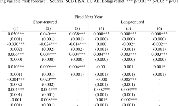
In Table 3, we report worker-level regressions in which the dependent variable is a
dummy variable that takes value 1 if a worker is fired within one year. The first set of
specifications in columns (1) to (4) does not contain the shock variable or its interactions.
The results are quite consistent across specifications. Short-tenured workers are more
likely to be fired at any point in time as the estimated likelihood of being fired is 6 to 7
percentage points higher for them. These effects are also very large in relative terms given
an unconditional probability of being fired of 6.2% across all workers. Constrained firms
are less likely to fire long-tenured workers than unconstrained ones in the regression with
firm fixed effects (column 2), while the RDD specification in Column (3) shows no
significant effect. The final result of the first four columns is that short-tenured workers are
more likely to be fired in constrained firms. The effect is large and significant and ranges
between 0.7% and 0.9%. Overall, these results are consistent with hypothesis 1.
Columns (5) to (8) of Table 3 show the fully interacted specification including
exchange rate appreciation shocks. The non-interacted coefficients follow the same pattern
as in columns (1) to (4). The shock variable is associated with a positive and significant
coefficient. Moreover, the interaction between shock and short tenure is negative and
significant. In other words, when a shock hits unconstrained firms, they deviate from the
LIFO policy and fire more long-tenured and fewer short-tenured workers relative to normal
times, confirming Hypothesis 3. The overall effect on firing is relatively small (under 1%
compared with a baseline firing rate of 6%). This is consistent with a temporary shock and
the identification of over-deviations from an industry-year average. However, the
composition of fired worker changes substantially in shock times for unconstrained firms.
34
allows unconstrained firms to fire the least productive workers across all tenure categories.
This effect also explains the result of the firm regressions, showing that tenure decreases
when firms are exposed to a shock. However, the next set of coefficients shows that this
broad firing effect is not present in financially constrained firms.
The effect of the shock for the firing of long-tenured workers by financially
constrained firms (the coefficient of Shock X Rating) is negative and significant. This result
is consistent with the model predictions that the costs of firing long-term workers are
higher for financially constrained firms. Finally, the interaction between short-tenured,
constrained and a negative shock has a clear positive coefficient across all specifications.
Financially constrained firms fire an abnormally large fraction of short-tenured workers
when they face a negative shock, confirming Hypothesis 4. The effect in columns (5) to (8)
ranges between 0.6% and 0.8%. This represents an increase of 10%-12.5% of the average
firing probability. Taken together, the results show that in normal times, the firing rate of
short-tenured workers is three times higher than that of long-tenured workers in
unconstrained firms (gold badge) but five times higher in constrained firms (bronze
badge). During shock times, the firing differential narrows down to a factor below two for
unconstrained firms, but the convergence of firing rates is absent for constrained firms.
The magnitude of these effects appears even more striking once put in perspective
with the size of the financing constraints captured by the rating. Given that we focus on
relatively healthy firms, the differences in access to credit across ratings are small. For
example, our estimates in Table A3 in Appendix 1 show increases with the average interest
rates paid between 0.16% and 0.30%. Alternatively, one can use, as benchmark, a
35
default of 35%, and the average default rates for each rating category. Such an exercise
yields differences in the average interest rates of 0.24% across gold-silver ratings and
0.78% across silver-bronze ratings. Junior loans could have a higher rate differential due to
lower recovery rates, but in any case, the effect is bounded between 0.37% for the
gold-silver transition and 1.21% for the gold-silver-bronze transition when we assume zero recovery
rates.9 Overall, the firms in our sample are financially healthy, although there are clear
differences in the interest rates they pay that signify their different degrees of credit
constraints.
6.3. Robustness checks
We run a number of robustness checks to confirm the results in the previous two
sections. Unless otherwise specified, the results and the details of the robustness checks are
shown in section EA2 of the External Appendix. We start with the definition of
constrained and shock. We explore the individual rating boundaries (gold-silver and
silver-bronze) and focus on firms in which a downgrade is most surprising (those that were Gold
for two years in a row before a downgrade). We also define the shock within a year using
the Shock (small) variable definition. The results of these alternative specifications are
consistent with the previous ones.
We then move on to the Firing variable. We consider two more stringent definitions of
firing: the first one requires as additional condition at least 180 days of unemployment.
The second one requires a drop in income of at least 10% when leaving the job. The results
are stronger under these stricter definitions (see Table EA5). Moreover, in Table 4, we
look at turnovers that are likely to be voluntary. We define voluntary as a turnover in
which a worker switches across firms and does not claim unemployment benefits in
9
36
between. This variable (also used in Baghai et al., 2016) should capture mostly voluntary
leaves and very few firings. When we use this definition of voluntary turnover instead of
firings, the main results no longer hold. The specifications with firm fixed effects in Table
4 show that after a demand shock, in a financially unconstrained firm, short-tenured
workers are actually more likely than long-tenured ones to voluntarily leave, thus reversing
the positive reallocation effect found using the fired workers indicator. Moreover, the triple
interaction coefficient is negative and significant instead of positive and significant.
Overall, these results suggest that any misclassification of voluntary leavers as fired
workers would actually dampen our results and is not driving them.
We also explore alternative tenure cuts to define short-tenured and long-tenured
workers who use either a three-year threshold to define short-tenured or definitions that
exclude workers of less than one year of tenure from the analysis. The results are, again,
consistent with those in the previous two sections (see Table EA6).
The effect of exchange rate shocks is potentially heterogeneous across firms if firms
are able to hedge their exposure through exchange rate derivatives. To rule out that this is a
factor affecting our results, we also run regressions (Table EA7) in which we exclude firms
with any financial assets (including derivatives). The results are robust to this exclusion.
Note also that when firms hedge, they tend to hedge their profits directly and not their
exports, so the marginal employment choices of hedged and non-hedged firms should be
the same.
7. Direct Evidence on Misallocation
The previous section shows evidence of firing policies being distorted by the presence
37
because more financially constrained firms fire an inefficiently large share of workers with
high productivity growth prospects. However, it is possible that other frictions not covered
by the model make financially unconstrained firms make suboptimal decisions that could
be attenuated by the presence of financing constraints. To rule out this possibility, in this
section, we aim to provide direct evidence of this misallocation by focusing on the quality
of workers who are fired and retained by constrained and unconstrained firms. We assess
the quality of workers using measures of their permanent productivity and their future
productivity. In particular, two productivity measures are calculated from separate wage
regressions: a worker’s predicted wage fixed effect and a worker’s expected wage growth.
We relate these measures to the firing policies of constrained and unconstrained firms
distinguishing between when they are in normal times and when they are experiencing
negative shocks.
7.1. Skill composition of fired and retained short-tenured workers
We explore the skill composition of short-tenured workers who are fired and retained.
We estimate a wage regression that includes a third-order polynomial on workers’ potential
work experience (age minus six minus years of education), year and firm fixed effects as
well as a worker fixed effect. The worker fixed effect can be interpreted as an estimate of
the worker’s time-invariant skills (see Abowd et al., 1999). We then run follow-up
regressions (reported in Table 5) in which the dependent variable is the average skill level
of short-tenure workers (average worker fixed effect) who are fired or retained in a given
year.10 The regressions follow a similar structure as the two first columns of Table 2, and it
10
The model has clear predictions about firms’ policies for firing short-tenured workers. The model also has predictions with respect to long-tenured workers, but these depend on the assumptions made about the productivity transitions between short-tenured and long-tenured workers. For this reason, we focus on short-tenured workers only.
38
is important to interpret both sets of results jointly, as the interpretation of the average skill
level of fired and retained workers depends on the firing intensity of the firm.
Columns (1) and (2) show the skill profile of short-tenured workers who are fired. The
first observed effect is that Shock is associated with a reduction in the skills of fired
short-term workers. The effect is sizeable, decreasing the average salary fixed effect of a fired
worker by 2.7% to 3%. The skill reduction is consistent with the results in Table 3; large
negative shocks are used by firms to fire across the tenure spectrum. More long-tenured
workers but fewer short-tenured workers are fired. The negative coefficient therefore
reflects that when fewer short-tenured workers are fired, those fired have lower skills (i.e.,
are more selected). More generally, if we think of tenure as a continuum, given that the
last-in-first-out pattern in firing is relaxed during negative shocks, we expect that the
firms’ sorting of workers relies less on tenure and more on productivity. As the sorting of
short-tenured workers according to their skill level becomes more pronounced, worse
workers get fired. This broad firing effect suggests that temporary negative shocks can
serve as a positive reallocation event in which unconstrained firms fire their less
productive workers across the tenure spectrum.
Next, the coefficient on Constrained is also negative and significantly different from
zero in the regression without firm fixed effects. This reflects the average skill-level effect
of fired workers in constrained firms relative to unconstrained firms during normal times.
Two counteracting effects are at work here. Constrained firms during normal times have
firing policies that are closer to a last-in-first-out rule. This would predict a positive
coefficient (more skilled short-term workers are fired). Simultaneously, as shown in Tables