Department of Economics Issn 1441-5429 Discussion paper 27/10
Immigrant and Native Saving Behaviour in Australia*
Asadul Islam1, Jaai Parasnis and Dietrich Fausten
Abstract
This paper examines whether the differences in the observed savings of immigrant and native households in Australia are related to underlying differences in observable characteristics of the two groups of households or to environmental factors. We use quantile regression and semi-parametric decomposition methods to identify the savings differential, and to isolate the factors that contribute to it. The basic finding is that while income can fully account for the observed difference in immigrant and native savings there are fundamental differences in the saving behaviour of the respective groups. Decomposition analysis suggests that the different characteristics of migrants and natives are
responsible for the observed difference in savings. The results also indicate that immigrants have a tendency to save more than natives when compared to Australian-born households of similar characteristics. These findings are consistent with the observed disparities in the wealth holdings of immigrant and native-born households in Australia.
Keywords: savings, immigrants, native-born, decomposition, Australia JEL classifications: F22, J61, D10
1 The corresponding author. Department of Economics, Monash University, PO Box 197, Caulfield East, Victoria 3145,
Australia; Tel: +61 3 99032783; Fax: +61 3 99031128; Email: [email protected].
* We thank Deborah Cobb-Clark, Steven Stillman, Chris Warwick and participants in the workshop on ―Consumption and Savingsԡ at Monash University and in the 2009 Australian Conference of Economists for their helpful comments and suggestions. The usual disclaimer applies.
© 2010 Asadul Islam, Jaai Parasnis and Dietrich Fausten
All rights reserved. No part of this paper may be reproduced in any form, or stored in a retrieval system, without the prior written permission of the author
Introduction
There is increasing evidence of disparities in the wealth and portfolio behaviour of immigrant
and native-born households (for example, Amuedo-Dorantes and Pozo 2002, Bauer et al.,
2007, Doiron and Guttmann, 2009 and Cobb-Clark & Hildebrand, 2006, 2009). Evidence presented in these studies of the existence of a sizeable gap between the stocks of wealth held by immigrant and native households naturally leads to an inquiry into the forces that generate this gap. Since the stock of household wealth constitutes the accumulation of savings flows it follows that saving behaviour is the fundamental driver of the observed differences in wealth holdings.
The literature typically attributes differential wealth holdings to differences in saving propensities with little regard to the specific circumstances and motivations that affect the two groups of households differentially. Unlike native households, immigrants have a greater opportunity and incentive for holding wealth abroad. Since their planning horizon extends by definition over (at least) two distinct geographical spheres, their wealth accumulation in only one of those spheres, their country of residence, is unlikely to provide a comprehensive view of immigrant wealth holdings. For instance, they may send remittances to support family and kinship or to fulfil social commitments. They may use their savings or bequests and inheritances to hold assets in the home country in the form of housing stock, capital investments, or even in very liquid form. Income uncertainty and the possibility of return migration in the face of adversity in the destination country provide incentives to build up
such asset holdings in the country of origin.1 Consequently, observed wealth differentials
within a particular jurisdiction are not necessarily indicative of different savings behaviours of immigrants and natives. The aim of this paper is twofold, to identify the respective saving patterns of immigrant and native households and to investigate the underlying determinants of savings. In particular, we explore whether there are systematic differences in saving behaviour across household groups. We then examine potential determinants of any observed differences in flows of saving and, hence, in wealth holdings.
The theoretical literature tends to favour the hypothesis that immigrants carry out more precautionary saving than natives and the resulting positive wealth differential in favour of immigrants (Amuedo-Dorantes and Pozo, 2002). Considerations in support of this position
1 Osili (2007) and Dustmann and Mestres (2009) provide detailed analyses of immigration and remittance
include the greater income uncertainty and more difficult access to welfare benefits typically faced by immigrants in host countries (Dustmann, 1997). The probability of return migration provides another motivation for strong saving (Galor & Stark, 1990; Dustmann, 1995). Geographic separation from family and friends makes it more difficult for immigrants to rely on their traditional networks for financial support in times of necessity. These factors provide potential incentives for immigrants to have higher precautionary saving rates than native households. Peer effects (Maurer & Meier, 2008) and inter-temporal time preferences (Browing & Crossley, 2001) may also promote such differential saving patterns.
The logical corollary of these conjectures, namely that immigrants have larger wealth
holdings than native households, is not supported by the existing empirical evidence. Bauer et
al. (2007) find that in 2002 immigrant households in Australia held approximately $18,000
less wealth than native households (at the median) after correcting for age and period since arrival. In the United States the median gap ($54,000) is approximately three times as large as in Australia, and it is more than seven times as large in Germany, exceeding $128,000. Cobb-Clark and Hildebrand (2009) and Doiron and Gutttmann (2009) corroborate the observed difference in the respective wealth holdings and asset portfolios of immigrant and native households in Australia. The basic problem is that this measured gap not only contradicts the a priori arguments but that it also is difficult to reconcile with the relative education advantage and other demographic characteristics of migrants. These attributes should
promote saving and lead to larger wealth holdings. According to Bauer et al (2007) these
characteristics are the main drivers of the wealth gap but they do not translate into a wealth advantage for immigrants. However, they may help to explain why the gap observed in Australia is relatively small.
Bauer and Sinning (2009) find that immigrants in West Germany save significantly less than natives. Their decomposition analysis indicates that this difference arises mainly from differences in observable socioeconomic characteristics (age, education, permanent income and the number of children) rather than differences in saving behaviour. They also find support for the Galor & Stark (1990) conjecture that the immigrant saving rate varies directly with the probability of return migration.
Labour market outcomes have an a priori ambiguous effect on saving patterns. Migrants in
2003) find that). While lower incomes tend to reduce saving, a higher probability of unemployment and greater sensitivity to adverse macroeconomic conditions are likely to stimulate precautionary saving (McDonald and Worswick, 1999). Immigrants and natives differ in terms of age, education and other demographic characteristics. For instance, in
Australia immigrants tend to have more years of schooling than natives (Antecol et al.,
2003), and a higher proportion are of working age. Life cycle variables can also account for differences between native and immigrant savings behaviour (Browning & Lusardi, 1996). Again, the net effect on relative saving performance is ambiguous, depending on the respective age distributions of the two populations.
The potential explanators for different saving patterns of migrant and native households suggested by the theory of saving behaviour and the migration literature can be grouped into two broad categories: factors that influence labour market outcomes, and cultural and institutional factors. The former include household-specific characteristics such as labour supply, educational attainment, family composition and life cycle considerations which influence labour force participation, employment and earnings. The latter include cultural practices, extended family obligations and differential access to formal and informal insurance arrangements to protect against shocks and possible reversal of the migration
decision (Bonin et al. 2009). Similarly, the socioeconomic strata in which migrants grew up,
the motivation for migration and the probability of return migration are potential
determinants of saving behaviour (Carroll et al. 1999). These cultural and institutional
influences are either specific to immigrants or they affect migrants and natives differentially (such as cultural practices). Some evidence of the influence on saving of country of origin and, hence, of the potential importance of social and cultural norms is provided in the
literature on the ―nativity gap‖. However, Carroll et al.(1994, 1999) obtain mixed findings for
Canada and the United States for the influence of cultural factors. They fail to identify any systematic differences by country of origin in the saving patterns of Canadian immigrants (1994) but they do observe such differences for US immigrants (1999).
In this study we first use Ordinary Least Squares (OLS) to identify the savings differential and to isolate the factors that contribute to the savings differential. The results indicate that differences in income of immigrants and natives can account for the observed differences in savings. In particular, when control for income we find that immigrants save more than natives – turning the finding from the raw data on its head. We then employ quantile
regression (QR) methods to identify the savings differential at different points of the conditional savings distribution. This enables us to describe the whole savings distribution and the relationship between savings and demographic and socio-economic characteristics as it evolves across its conditional distribution. The results of the QR analysis are similar to the OLS estimates.
Next we apply the quantile based decomposition technique of Machado and Mata (2005) to analyse the difference in savings between immigrants and natives. This method involves estimating quantile regressions on savings for immigrant and native households, and then constructing a counterfactual distribution of immigrant savings using the distribution of native covariates. This counterfactual distribution estimates the distribution of immigrant savings that would have occurred had immigrants been endowed with the distribution of native household characteristics (but behaved like immigrants). By identifying the ―migrant‖ returns to ―native‖ characteristics the counterfactual distribution isolates the consequences of ―immigrant behaviour‖. The decomposition method thus allows us to isolate the effects of the differences in the distributions of immigrant and native characteristics from the differences in the returns to those characteristics. Its substantive finding is that the diverse characteristics of immigrants and natives explain the savings gap. Immigrants have a tendency to save more than natives, giving rise to positive conditional differences (holding income and other characteristics fixed) in savings behaviour when compared to natives.
Data and Descriptive Statistics:
We use data from the Australian household expenditure surveys (HES) for 1988/89, 1993/94, 1998 and 2003/04. The HES data provide detailed information about the expenditure, income and household characteristics of a sample of households resident in private dwellings throughout Australia. The data allows investigating the savings behaviour over a significant period of time. Since household surveys rarely report a direct, robust and consistent measure of savings it is necessary to construct a savings series from data on income and consumption. Savings can be measured either as flow changes in the stock of wealth or as the difference between income and consumption flows. We use flow measure of household level savings considering the cross-sectional nature of the dataset. We focus on out-of-pocket saving, defined as the difference between consumption and after-tax income. This definition, in turn, requires accurate treatment of income and consumption in the presence of capital gains, mortgages, pension funds and accounting for the durable nature of some consumption items.
Income: Income comprises cash and in-kind receipts of a regular and recurring nature. It is the sum of wage and salary disbursements, tips, other labour income, farm income, business income (net proprietor‘s income from unincorporated business), net rental income, interest on
savings and dividends, and transfer income from government, private institutions and other
households, employer and employee contributions to pension funds, inheritance, gifts and other income from family members. Disposable income is defined as total household income minus taxes.
Capital gains: We exclude all capital gains and losses from household income. Differentiating between unrealized and realized gains is problematic, while including capital gains in the estimates of savings would be difficult because of the high degree of volatility of this component. Therefore, we consider the ―active‖ component of saving to be represented
by the difference between income exclusive of capital gains, and consumption.2
Consumer durables: Their appropriate treatment, as consumption or investment expenditure, has long been controversial. Consumer durables are typically treated as final consumption expenditure when purchased by households. Alternatively, the fact that they generate a stream of future services or income that raises future consumption possibilities suggests they should be treated as investment expenditure. Since total outlay on consumer durables is not insignificant, and since their services satisfy consumption demand, there is merit in recognising net acquisitions of consumer durables in consumption spending while also acknowledging their investment role.
We apply the perpetual inventory method to obtain an estimate of expenditure for the year
that corresponds to the stock ofconsumer durables (Jalava and Kavonius, 2009). In view of
the underlying ambiguity, and also in order to analyse the sensitivity of our estimates, we use three alternative specifications of consumption, each including car registration and insurance fee as 100 percent expenditure for the year, with corresponding specifications for savings (Sav1-Sav3).
(1) C1 includes all expenditure on consumer durables for the survey year;
2
We acknowledge that capital gains, even unrealized capital gains, can influence saving through the so-called ‗wealth effect‘. This is illustrated, for instance, by the consumption boom prior to the global financial crisis. The stock market boom had sustained massive increases in spending by reducing the saving rate as households treated capital gains as a substitute for savings.
(2) C2 includes an imputed value of consumer durables corresponding to a flat 15 percent depreciation of the stock;
(3) C3 excludes all consumer durables and treats them as investment. This definition uses
only items purchased for the year, and applies the depreciation method.3
Housing expenditure: Rent paid by households is included in consumption expenditure. Treatment of housing expenditure for owner-occupier households is more complex since they consume equivalent housing services without paying rent while building up equity in real estate. In recognition of this dual effect mortgage service payments can be decomposed into amortisation, which is treated as saving, and interest which is considered as consumption expenditure. Following Dynan et al. (2004), we treat gross imputed rent as the corresponding housing expenditure. The 2003-04 survey reports experimental estimates of imputed rents for owner-occupied dwellings. Imputed rents for earlier survey years are estimated by applying the methodology detailed in ABS (2008). Imputed rent is calculated using a hedonic model where rent is a function of the location and dwelling characteristics and the Inverse Mills ratio. The Inverse Mills ratio is obtained from a probit model controlling for the characteristics of the occupants.4
Consumption expenditure: Consumption equals total household expenditure plus imputed
rent for home owners less the sum of: mortgage amortisation payments, expenditure on home
capital improvement, life insurance payments, and spending on new and used vehicles including running costs (petrol, insurance, registration). This implies that expenditure for houses and vehicles are part of savings in this definition.
Pension and Superannuation: Contributions to pension plans are counted as transfers from governments to households. Household, and employer, contributions to private pension plans in expectation of a future pension are counted as savings and income, respectively. It follows that benefits paid by the plans to retirees are excluded from personal income because they draw down savings balances accumulated in the plan much like withdrawals from a bank account built up by retirees. Only the contributions made to the plan are regarded as income (the earnings of the plan are not income). In contrast, benefits obtained by households from
other sources such as child/age care benefit are transfer receipts and, hence, income.
3
Household durables and semi-durables are defined as consumption goods that might be used several times or continuously over a period of 2-3 years or longer. Durables include, inter alia, motor vehicles, furniture, cookers, fridges, washing machines, television sets, musical equipment, computer equipment, watches and jewellery. Semi-durables include, inter alia, clothing, footwear, household utensils, equipment for sport and books. Non-durables include food, beverages, tobacco, pharmaceutical products, petrol, cosmetics, newspapers etc.
4
INSERT TABLE 1 HERE
Descriptive statistics for migrant and native households from the four expenditure surveys are reported in Table 1. Both savings and income are reported in current Australian dollars per week. The income differential between the two groups is moderate throughout the period, changing from approximately 0.8% in favour of migrants (in 1988/89) to 3.6% in favour of natives (in 2003/04). With the exception of 1993/94 migrants consistently save less than natives, although the difference in 1998 is nugatory. Notably, when migrants enjoyed a positive income differential in 1988/89 they saved less than natives. It is also notable that the savings differential is robust with respect to the amount of consumer durable expenditure included in savings (Sav2 and Sav3). Conversely, when no durable expenditure is included in savings (Sav1) we observe insignificant weekly dis-savings by migrants in 1988, but significant and positive savings in 2003. Table 1 shows that both savings differential and income differential are increasing over time. Migrant household heads are consistently older than native household heads, with the age difference approximately doubling over the observation period. Migrant households are less likely to have a female head or to be a sole parent, and they are typically larger than native households.
We use a kernel smoothing technique to estimate the savings distribution for each year in order to describe the immigrant-native savings differentials across the distribution. These distributions are plotted in Figures 1A-1D. In 2003 the savings distribution of natives is slightly to the right of the immigrants‘ distribution. No such consistent distributional difference is apparent in the earlier years. They are almost identical in 1988 although the natives‘ distribution tends to be slightly to the right in 1993.
INSERT FIGURE 1 HERE
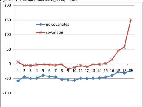
Figures 2A-2D display the difference in weekly savings between immigrants and natives at different quantiles. We also include unconditional quantile regression coefficients for different quantiles following Firpo (2007). The method allows estimating the unconditional quantile of savings while allowing covariates to match immigrants and natives. We include covariates in the first stage regression to estimate a propensity score for each household. That propensity score is then used as weight in estimating the unconditional savings at different quantiles. That is, we reweight the empirical distribution of the outcome variable using weights that equalize the empirical distributions of the explanatory variable. The raw data
estimates of quantiles in 2003 (Figure 2A) indicate that immigrants save considerably less than natives at each quantile of the savings distribution. However, when we use covariates to match immigrants and natives we find that the savings gap is reduced (in absolute terms) at each quantile, and that it turns positive at higher levels. Immigrants save more than natives at the 80th or upper quantile. In the intermediate years (1993 and 1998) the raw estimates of quantiles suggest that immigrants, in general, save more than natives above the median of the savings distribution but that otherwise they save less. After reweighting (using covariates) we find that the savings gap (in favour of natives) decreases across the entire distributions in 1988 and 1998. In 1988 immigrants saved more than natives above the median of the savings distribution while a decade later they did so along the entire distribution. The corresponding estimates for immigrant savings in 1993 exceed natives‘ only at the 85th quantile or above. The results indicate that a large part of the positive raw savings differential can be accounted for by the characteristics of households. They also indicate similarities in the raw savings differential between 2003/04 and 1988 as well as between 1993 and 1998. Thus, while there is a convergence of savings from 1988 to 1993 and 1998, at least above the median of the distribution, we see the trend reverse in 2003/04. That pattern is qualitatively consistent with the trends displayed by the three sets of savings figures presented in the descriptive statistics.
INSERT FIGURE 2 HERE Empirical Strategy:
Our general approach to compare the saving patterns of immigrant and native households is to estimate functions of the following form:
i i i i X M S
1
2
(1)where subscript i refers to household, X is a vector of household demographic and
socio-economic characteristics including income, M is a dummy variable equal to one if a
household head is born overseas and zero otherwise. S is the savings variable. We use the flow of savings rather than the saving rate or propensity to save as many low income households have high dis-savings that may dominate the resulting estimates.
β2 in equation (1) is an estimate of the savings differential between immigrant and native households using OLS. Sample selection is not a problem for our savings model since savings are either positive or negative depending on income and consumption. Since income
is the most important determinant of saving, we examine in detail its effect on the size of coefficient β2. The main objective is to ensure that observed differences in savings are not incorrectly attributed to differential saving behaviour when in fact they reflect differences in household income. We also consider the heterogeneity of saving behaviour across age groups since savings are likely to vary over the life cycle. For example, Attanasio (1998) finds that a typical age profile displays a pronounced hump, peaking around age 55. The saving-age profile could be an important explanatory factor in the present setting as immigrants face an extended transition period on arrival in Australia. Further, immigrants tend to be older than natives (Table 1). We, therefore, divide the sample of households into three distinct age groups: 20-35 years, 35-55 years, and 55-70 years.
OLS estimates of β2 measure the mean or average savings differential conditional on X. It is
not suitable in the presence of the skewed distributions that typically characterise savings data. A large number of households do not save at all, and their proportions are likely to differ between natives and migrants. It is likely that exogenous variables determine not only the mean but that they also influence other interesting parameters of the conditional distribution of the dependent variable (Koenker and Basset, 1987). We, therefore, use the quantile regression (QR) approach introduced by Koenker and Bassett (1978) to examine the
heterogeneity of saving behaviour.5 QR allows parameter estimates of the marginal effects of
the explanatory variables to differ across the quantiles of the dependent variable. This means that at each point of the distribution QR can control more fully for differences between the savings of immigrants and natives that are attributable to their respective characteristics. Since QR allows the savings differential to differ across quantiles, the reported results are unlikely to be dominated by some extreme values of savings which could bias OLS results.
The basic QR model specifies the conditional quantile as a linear function of covariates.
Following Buchinsky (1998), we specify the θth conditional quantile of the savings
distribution for the ith household (i=1,2,...N) as:
(2) ) 1 , 0 ( ) | ( , i
i i i i
i X M u Quant S x x S 5The estimation process of QR is similar to that of OLS in that parameter estimates are derived through minimization of errors. However, QR measures least distance of weighted absolute values of the errors whereas OLS measures least distance of the sum of the squared errors.
where Xi is a vector of exogenous variables, M is the immigration dummy variable, the
coefficient vector βθ represents the returns to covariates at the θth quantile, and γθ is the main
parameter of interest. Quant(Si | Xi)denotes the quantile of Si, conditional on regressor
vector Xi. The θth regression quantile (0<θ<1) of s is the solution to minimizing the sum of
absolute deviation residuals:
(3) | | ) 1 ( | | 1 min : :
i i x yi i iyi x i i i i X M S X M S nSince the minimization problem of equation (3) has no explicit form it is solved with linear programming methods. We estimate standard errors of the estimates by bootstrapping with 500 repetitions. Estimates of quantile regressions are interpreted like OLS regression estimates: they represent the marginal effect of covariates on the θth quantile of savings.
Decomposition:
Regressions based on equations (1) and (3) assume that β1 is equal for immigrant and native
households within a given quantile of savings distribution. This contradicts our working hypothesis that the savings behaviour of the two groups of households may differ, i.e., that
they respond differently to the exogenous factors included in X. Since the estimated β1‘s are
disproportionately influenced by the Australian-born groups which comprise the majority of the population they reveal little information about the behaviour of immigrants. At the same time, the distribution of migrants and natives with equal characteristics may differ significantly across job types. Superior knowledge of local labour markets as well as local experience and networks enable a native worker to obtain a better job than an equally qualified migrant worker. That is, compared to a migrant worker, a native worker may be
able to command higher returns for a given set of characteristics, 𝑋𝑖 . Green et al. (2007) find
that immigrants are more likely to be overeducated, that is, to be working in low-skilled occupations relative to their qualifications than natives. Since the potential returns to education and job experience may differ between the two groups they are also likely to affect the savings differentials. These returns reflect the differential income streams derived by migrant and native workers from a given set of characteristics X. In order to isolate the respective influence of characteristics and behaviour we decompose the savings differential.
The conventional decomposition method introduced by Blinder (1973) and Oxaca (1973) identifies the source of the difference between the means of two distributions. However, as
noted above, means are not particularly informative moments when distributions are skewed. Rather, it is necessary to decompose the entire density of the savings distributions. To that end we employ a decomposition procedure based on the quantile regression approach. Some alternative methods that focus on the entire distribution (see, for example, DiNardo, Fortin and Lemieux, 1996; Autor, Katz, and Kearney, 2008; Firpo, Fortin and Lemieux, 2009) are currently used in the wage inequality literature. We use the quantile-based decomposition method proposed by Machado and Mata (2005) which has gained popularity in recent studies (for example, Nguyen et al., 2007; Albrecht et al., 2003; Arulampalm et al., 2007). It enables us to decompose the immigrant-native savings differential at each quantile into two components: one component which is due to intergroup differences in the distribution of covariates (characteristics), and another which reflects the differences in the distribution of returns. That is, the decomposition enables us to identify the extent to which the savings gap can be attributed respectively to the different characteristics of natives and migrants and to the differences in their savings behaviour. (The later corresponds to the ‗return factor‘ in the wage inequality literature).
The basic idea of the Machado and Mata (2005) decomposition approach is to estimate the whole conditional distribution of savings by a quantile regression, and then to integrate the conditional distribution over the range of covariates in order to obtain an estimate of the unconditional distribution. It is then possible to estimate counterfactual unconditional distributions to perform the usual decompositions. We are particularly interested in the following counterfactuals:
i. the immigrant savings density function that would arise if immigrants had the same
characteristics as natives. This enables us to identify the coefficient effect which is
also known as the returns or savings structureeffect
ii. the density function that would arise if immigrants had the same returns to
characteristics as natives. This enables us to determine the covariate effect, which is
also known as the composition or endowmenteffect.
We construct the counterfactual savings distributions of natives and migrants, respectively, as follows:
(1) Estimate quantile regression coefficients βm for each quantile θ=0.01, 0.02,...0.099,
(2) Use the natives data to generate the fitted values S*(θ)=Xaβm(θ). For each θ this
generates Na fitted values, where Na is the size of the native sub-sample.
(3) Select n elements at random from the elements of S*(θ) for each θ and stack these into a 99×n element vector S*. The empirical CDF of these values is the estimated counterfactual distribution of natives.
(4) Estimate immigrant counterfactual density by reversing the roles of immigrant and
native data in steps 1 and 2. That is, use the native dataset to estimate the quantile regression coefficient and generate the bootstrap data from the immigrant dataset.
Let Sm(θ) and Sa(θ) represent the θth quantile of the immigrant and native distributions. Then
the difference between their savings distributions at the θth quantile is given by:
Sm(θ)- Sa(θ)= {Sm(θ)- S*(θ)}+ {S*(θ)- Sa(θ)}. (4)
We use the immigrant counterfactual density to obtain: Xmβm(θ)- Xaβa(θ)= Xmβm(θ) –Xaβm(θ)+ Xaβm(θ) –Xaβa(θ)
=Xa{βm(θ)- βa(θ)}+βm(θ){Xm –Xa} (5)
The first term on the right hand side of equation (5) represents the returns or savings
structure or coefficient effect: it measures the contribution to the migrant-native savings gap
at the θth quantile of differences in the returns obtained by migrants and natives with
hypothetically identical characteristics. The second term on the right hand side is the
covariate or endowment or composition effect: it measures the contribution of the different characteristics (covariate values) of immigrant and native households to the savings gap at
the θth quantile. In contrast to the wage inequality literature, the savings structure effect is a
little difficult to interpret. It reflects the consequences of unknown dimensions of behaviour, having accounted for household socio-economic characteristics. Possible factors that could contribute to the savings structure effect include the difference, by nativity status, in household spending on human capital, particularly on investment in children‘s education. Card (2005), for example, finds that immigrant households invest more in their children‘s education. Another factor is the role of interfamily assistance in smoothing consumption. The development literature (for example, Islam and Maitra (2009)) notes that consumption smoothing takes place at the community or village level, or between kinship level. Since most recent immigrants originate predominantly from developing countries, differences between immigrants and natives in their reliance on nonmarket methods of support and financial assistance may account for systematic savings differences by nativity status. A third factor
comprises differences in attitudes or preferences regarding wealth accumulation. For example, it is probable that the very different experiences of immigrants and natives may give rise to different levels of risk aversion or distrust towards institutions, financial and
others.6 We leave these conjectures for future research. For present purposes we interpret the
savings structure or returns effect as reflecting differential preferences or attitudes towards saving by immigrant and native households. These behavioural differences may reflect a combination of the factors mentioned above as well as other influences.
Results:
INSERT TABLE 2 HERE
Table 2 presents OLS estimates of equation (1). In particular, it shows the effect of the
nativity status variable on different measures of weekly household savings (2). The
estimated coefficients represent immigrant relative to native household saving. They are reported for the four survey years with (even numbered columns) and without (odd numbered columns) controlling for income. The regressions also include household demographic and socio-economic characteristics such as, age, sex, marital status, education, employment status of household head, number of children and number of adults, and type of family (nuclear or joint). It also includes state fixed effects to capture variation across different geographic locations. The results show that immigrant households save considerably less than natives when all other variables but income is included. Including income as a control, however, changes the situation significantly—immigrants consistently save more than natives, both at the level of the household and per capita.7 That difference has remained roughly constant throughout the period of observation. Conversely, when we do not control for income we observe highly significant substantial savings gaps in favour of Australian-born. For example for 2003, column 1 of Table 2 indicates that immigrant households save $40-$55 less per week than natives. On the other hand, column 2 which controls for income records positive savings differentials in favour of immigrants of $19-$25 per week. The results overwhelmingly support the fact that measured immigrant savings are smaller than savings by natives. But that difference is largely attributable to differences in income. When we control for income we obtain the opposite results of a savings gap in favour of immigrants. Table 2 also indicates that this conclusion is robust with respect to different measures of savings that reflect different treatments of expenditure on consumer durables. In the
6 Barsky et al. (2002) provide a similar argument of wealth accumulation by blacks and whites in America.
7
following, we only report results for the savings measure that includes durable expenditure (Sav3).
INSERT TABLE 3 HERE
Table 3 reports coefficients of the immigrant dummy for different age groups using the full set of characteristics, including income. We split the sample according to the age of the household head as reported in the survey. We group households into different age categories since a considerable proportion of immigrants are at their transitional stages. This would also reduce the impact of labour market entry and exit. It is immediately apparent that relative immigrant savings are not consistent across age groups or over time. Abstracting from the 1993 figures, relative savings by the young have decreased over time, both at the household level and per capita. Savings of the middle group (age 35-55) and old group (55-70) have trended upwards along an inverted U-shape, decreasing from 1998 to 2003. While most immigrants save more than natives when conditioning on income and other characteristics, it is the younger immigrants who in recent years are saving less than the native-born. This age group would have arrived recently in Australia. Compared to their local counterparts, they face considerable challenges to settle and assimilate in Australia. It is, therefore, not surprising that their savings are lower compared to young native Australians.
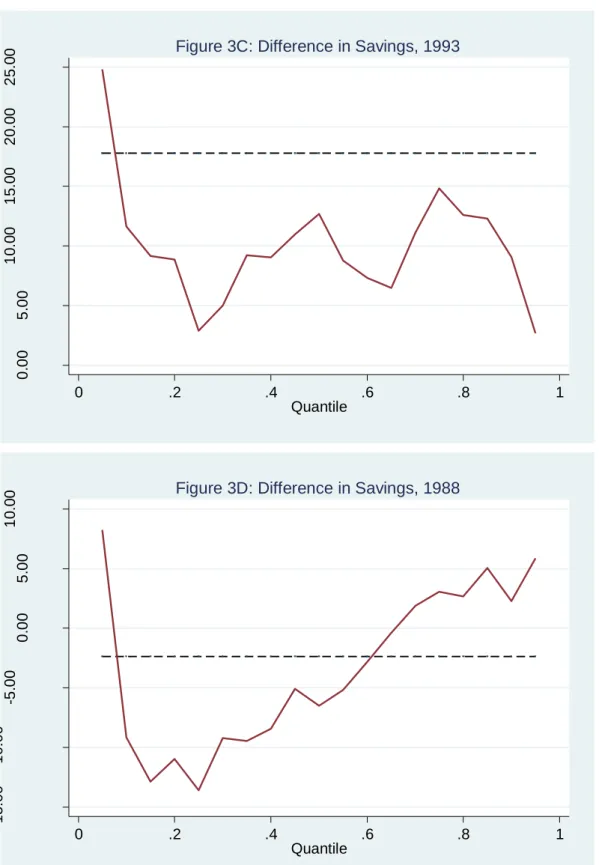
INSERT TABLE 4 HERE INSERT FIGURE 3 HERE
Table 4 reports conditional (on income and other regressors) quantile regression estimates following Koenker and Bassett (1978). With the exception of 1988, immigrant households save more at each quantile of the savings distribution. The savings differential is generally larger above the median of the distribution (except in 1998 when the largest difference is
observed at 25th quantile), and that difference is increasing with time. For example, at the 75th
quantile, the immigrant-natives weekly conditional savings difference is only $3.05 in 1988. By 2003 that difference has increased more than five-fold to $17.43. The estimation results based on per-capita savings reveal a similar picture. Immigrant households‘ per-capita
weekly saving at the 90th percentile in 1988 was $6.8 higher than that of natives. By 2003,
that differential had more than doubled, to about $14.
The fundamental finding is that immigrants save more than natives along virtually the entire distributions for each observation year. Even poor immigrant households save more than their
native counterparts, except for 1988. Figures 3A-3D plot the estimates of the (conditional) quantile regression coefficients for each percentile of the savings distribution. The dashed lines represent the coefficient estimates obtained from the OLS regressions. The figures show
that all the coefficients are positive with exceptions occurring in 1988 for the lower half of
the distribution and in 2003 below the 30th quantile. This means that the conditional savings of immigrants exceed natives‘ savings at each percentile of the savings distribution.
INSERT FIGURE 4 HERE
The results from Machado-Mata decomposition are depicted in Figures 4A-4D. The effects of characteristics or composition effects associated with an X variable correspond to the term
βm(θ)(Xm –Xa). It represents the component of the savings differential that is due to
differences in characteristics. Similarly, the effects of coefficient or the structure effects are
captured by the term Xa(βm(θ)- βa(θ)). This represents the difference in the returns obtained
by immigrant and native households with given characteristics which we attribute to behavioural differences in savings. Figure 4A, for example, shows that the raw savings gap in
2003 favours natives until about the 95th percentile. The figure shows that the role of
characteristics/covariates in explaining the savings gap increases as we move up along the savings distribution. The decomposition analysis demonstrates that the negative savings gap is attributable to the different characteristics of the two groups of households. It also indicates that the differences in characteristics between immigrants and natives alone can account for more than the observed raw differences in savings. If immigrants and natives had identical characteristics the former would have saved more than the latter. The differences in characteristics matter more at the upper quantile than in the lower ones. The behavioural differences in savings are also stronger in the top quartile. This means that among the poorer households, differences in household characteristics matter more than the differences in returns to those characteristics. On the other hand, dominance of returns effects at the upper end of the distribution means that richer immigrant households display a relatively strong preference towards savings.
The decomposition results for 1998 indicate that raw saving differences become positive
beyond the median, and they are clearly significant after the 60th quantile. The figure shows
that the savings gap can be attributed mostly to the differences in characteristics, and that the total difference in savings and the composition effect move in parallel. The composition
effect, which captures the savings gap associated with observable characteristics (X), is
very flat curve for behavioural differences across the entire distribution, indicating that this difference is roughly constant across the different groups of households. We observe a similar pattern in 1993 and 1988 (Figures 4C and 4D, respectively). In 1993 the raw savings difference becomes positive in the vicinity of the median, and there is a sharp increase towards the end of the distribution. The difference is, however, explained well by the differences in characteristics. The saving difference in 1988 is fully explained by differences
in characteristics after the 40th quantile, and the returns effects or behavioural differences is
almost zero for the corresponding part of the distribution.
Overall, we find that differences in characteristics drive differences in savings, and these differences have become increasingly important in recent years. The returns effect has also contributed increasingly to the change of the savings differential in favour of migrant households. To the extent that the returns effect reflects behavioural differences, immigrants tend to display increasing preferences towards saving.
Our main finding across OLS, QR and semi-parametric decomposition analyses is that differences in the observed characteristics of migrant and native households account for relatively lower migrant saving. However, given these characteristics, particularly income, migrants have a consistently higher propensity to save than native households. This result is consistent with the recent findings that immigrants hold less wealth than natives (Doiron & Guttman, 2009; Cobb-Clark & Hilderbrand, 2009) notwithstanding a stronger disposition to save.
Conclusion:
At the most basic level, our results indicate that both sets of explanatory variables – labour market outcomes and cultural and institutional factors - are important determinants of the nativity saving gap. Labour market outcomes, specifically income, are the single most important determinant of the observed savings gap in favour of native households. At the same time, demographic and other characteristics play a significant role in explaining the differential saving behaviour of immigrant and native households. In fact, our analysis suggests that immigrant households tend to save more than native households when we control for these characteristics, and that this property characterizes the entire savings distribution. However, the savings differential is not invariant across the entire savings distribution: it is higher at the upper end of the savings distribution. At the same time, the
results suggest some heterogeneity in immigrant saving behaviour: recent younger immigrants tend to save less than their native counterparts, even conditioning on income. However, anecdotal evidence suggests that younger immigrants also make larger remittances to their home country compared to their older counterparts.
The fundamental finding of a positive savings gap in favour of immigrants applies to household as well as per capita saving. It is robust over time and across different treatments of consumer durables reflected in the alternative specifications of consumption spending. Thus, the raw savings and wealth data obscure important differences in underlying saving behaviour. To the extent that saving behaviour is a consideration in the formulation of immigration policy the raw data should be treated with care and circumspection. On the positive side, policies that facilitate the labour market assimilation of migrants are likely to yield a nontrivial dividend in promoting national savings and, thus, easing the pressure on Australia‘s current account balance.
References
ABS (2008), ―Experimental Estimates of Imputed Rent, Australia” Cat. No. 6540.0, Austrlian
Bureau of Statistics, Canberra.
Albrecht, J. W., Bjorkland, A., & Vroman, S. B. (2003), ―Is There a Glass Ceiling in
Sweden‖, Journal of Labor Economics, 21(1), 147-177.
Antecol, H., Cobb-Clark, D., & Trejo, S. J. (2003). ―Immigration Policy and the Skills of
Immigrants to Australia, Canada and the United States‖, Journal of Human Resources, 38(1),
192-218.
Amuedo-Dorantes, C. & Pozo, S. (2002) ―Precautionary Savings by Young Immigrants and
Young Natives‖, Southern Economic Journal, 69, 48-71.
Arulampalam, W., Booth, A. L., & Bryan, M. L. (2007), ―Is There a Glass Ceiling over
Europe? Exploring the Gender Pay Gap Across the Wage Distribution‖, Industrial and Labor
Relations Review, 60(2), 163-186.
Attanasio, O. (1998), ―A Cohort Analysis of Saving Behaviour by US Households‖, Journal
of Human Resources, 33(3), 575-609.
Attanasio, O., Berfloffa, G., Blundell, R., & Preston, I. (2002) ―From Earnings Inequality to
Consumption Inequality‖, The Economic Journal, 112, C52-C59.
Autor, D. H., Katz, L. F., & Kearney, M. S. (2008), ―Trends in U.S. Wage Inequality:
Revising the Revisionists‖, The Review of Economics and Statistics, 90(2), 300-323.
Barsky R. ,Bound J., Charles K.K. & Lupton J.P., (2002), ―Accounting for the Black-White
Wealth Gap: A Nonparametric Approach”, Journal of the American Statistical Association,
American Statistical Association, 97, 663-673.
Bauer, T. K., Cobb-Clark, D. A., Hildebrand, V. A., & Sinning, M. (2007) ―A Comparative Analysis of the Nativity Wealth Gap‖, ANU Centre for Economic Policy Research Discussion Paper No. 554.
Bauer, T. K., & Sinning, M. G. (2009). ―The Savings Behavior of Temporary and Permanent
Migrants in Germany‖, Journal of Population Economics, forthcoming.
Blinder, A. S. (1973), ―Wage Discrimination: Reduced Form and Structural Estimates‖,
Journal of Human Resources, 8, 436-455.
Bonin, H., Constant, A., Tatsiramos K., & K. F. Zimmermann (2009) ―Native-Migrant
Differences in Risk Attitudes‖, Applied Economics Letters, 16(15), 1581-1586.
Browing, M. & Crossley, T. (2001) ―The Life-cycle Model of Consumption and Saving‖, The
Journal of Economic Perspectives, 15, 3-22.
Browning, M., & Lusardi, A. (1996). Household Saving: Micro Theories and Micro Facts.
Journal of Economic Literature, 34(4), 1797-1855.
Card, D. (2005). ― Is the New Immigration Really so Bad?‖, Economic Journal, 115(507),
F300-F323, November
Carroll, Christopher D., Rhee, C., & Rhee, B. K. (1994), ―Are There Cultural Effects on
Saving? Some Cross-sectional Evidence‖, The Quarterly Journal of Economics, CIX(3).
Carroll, Christopher, Â D., Rhee, B. K., & Rhee, C. (1999), ―Does Cultural Origin Affect
Saving Behavior? Evidence from Immigrants,‖ Economic Development and Cultural
Cobb-Clark, D. A. (2003) ―Public Policy and the Labor Market Adjustment of New
Immigrants to Australia‖, Journal of Population Economics, 16, 655-681.
Cobb-Clark, D. A., & Hildebrand, V. A. (2009). ―The Asset Portfolios of Native-born and
Foreign-born Households‖, Economic Record, 85(268), 46-59
Cobb-Clark , D. A. & Hildebrand, V. A. ( 2006). ―The Wealth And Asset Holdings Of
U.S.-Born And Foreign-U.S.-Born Households: Evidence From SIPP Data,‖ Review of Income and
Wealth, 52(1), 17-42.
DiNardo, J., N. M. Fortin, et al. (1996). ―Labor Market Institutions and the Distribution of
Wages, 1973-1992: A Semiparametric Approach.‖ Econometrica 64(5): 1001-1044.
Doiron, D., & Guttmann, R. (2009). ―Wealth Distribution of Migrant and Australian-born
Households‖, Economic Record, 85(268), 32-45.
Dustmann, C. (1997), ―Return Migration, Uncertainty and Precautionary Savings‖, Journal of
Development Economics, 52, 295-316.
Dustmann, C. (1995) ―Savings Behavior of Return Migrants‖, Zeitschrift für Wirtschats-und.
Sozialwissenschaften (ZWS), 115, 511-533.
Dustmann, C. & Mestres, J (2009). ―Remittances and Temporary Migration,‖ CReAM Discussion Paper Series 0909, Centre for Research and Analysis of Migration (CReAM), Department of Economics, University College London
Dynon, K. E., Jonathan, S., & Zeldes, S. P. (2004). ―Do the Rich Save More?,‖ Journal of
Political Economy, 112(2), 397-444.
Firpo, S. (2007), ―Efficient Semiparametric Estimation of Quantile Treatment Effects‖,
Econometrica, 75(1), 259-276.
Firpo, S., Fortin, N., & Lemieux, T. (2009), ―Unconditional Quantile Regressions‖,
Econometrica, 77(3), 953-973.
Galor, O., & Stark, O. (1990), ―Migrants' Savings, the Probability of Return Migration and
Migrants' Performance,‖ International Economic Review, 31(2), 463-467.
Green, C., Kler, P. &Leeves, G. (2007), ―Immigrant Overeducation: Evidence from Recent
Arrivals to Australia, Economics of Education Review, 26(4), 420-432.
Islam, A., and Maitra, P. (2009), ―Health Shocks and Consumption Smoothing in Rural Households: Does Microcredit have a Role to Play?, Working Paper, Monash University Jalava, J., & Kavonius, I. K. (2009), ―Measuring the Stock of Consumer Durables and its
Implications for Euro Area Savings Ratios‖, Review of Income and Wealth, 55(1), 43-56.
Lee, S. (2007). "Endogeneity in quantile regression models: A control function approach."
Koenker, R., & Bassett, G. (1978), ―Regression Quantiles‖, Econometrica, 46, 33-50.
Koenker, R., & Bassett, G. (1987), ―An Empirical Quantile Function for Linear Models with
IID Errors,‖ Journal of the American Statistical Association, 77, 407-415
Maurer, J., & Meier, A. (2008) ―Smooth it Like the ‗Joneses‘? Estimating Peer-Group Effects
in Intertemporal Consumption Choice‖, Economic Journal, 118, 454-476.
Machado, J. A. F., & Mata, J. (2005), ―Counterfactual Decomposition of Changes in Wage
Distributions Using Quantile Regression‖, Journal of Applied Econometrics, 20(4), 445-465.
McDonald, J. T., & Worswick, C. (1999), ―The Earnings of Immigrant Men in Australia:
Assimilation, Cohort Effects and Macroeconomic Conditions‖, Economic Record, 75, 49-62.
Miller, P. W., & Neo, L. M. (2003), ―Labour Market Flexibility and Immigrant Adjustment‖,
Economic Record, 79, 336-356.
Nguyen, B. T., Albrecht, J. W., Vroman, S. B., & Westbrook, D. M. (2007), ― A Quantile
Regression Decomposition of Urban-Rural Inequality in Vietnam‖, Journal of Development
Economics, 83(2), 466-490.
Oaxaca, R (1973). ―Male-Female Wage Differentials in Urban Labor Markets‖, International
Economic Review 14(3): 693-709.
Osili, O. (2007). ―Remittances and savings from international migration: Theory and
evidence using a matched sample‖, Journal of Development Economics, 83(2), 446-465,
Table 1: Descriptive Statistics
Variables 2003/04 1998 1993/94 1988/89 Migrants Natives Migrants Natives Migrants Natives Migrants Natives
Savings: Sav1 74.20 (620.69) 109.30 (564.31) 0.60 (447.65) 6.19 (406.54) -25.54 (398.65) -33.43 (362.83) -15.24 (338.08) 17.27 (346.68) Sav2 207.76 (598.10) 250.33 (530.83) 103.46 (415.68) 107.79 (376.76) 57.30 (375.35) 49.88 (334.66) 56.18 (309.46) 82.63 (324.69) Sav3 215.35 (598.76) 258.25 (531.53) 121.61 (416.59) 125.72 (378.71) 71.91 (377.21) 64.59 (335.89) 68.79 (310.36) 94.16 (325.75) Disposable income 1027.80 (750.94) 1065.28 (717.33) 721.68 (511.05) 722.12 (496.37) 622.78 (483.34) 596.93 (415.49) 514.90 (366.02) 510.94 (395.46) Age 51.01 (15.21) 47.88 (16.11) 48.95 (14.30) 45.56 (15.74) 48.43 (15.29) 46.09 (16.78) 47.70 (15.06) 46.20 (16.80) Sex (female) 0.38 (0.48) 0.41 (0.49) 0.36 (0.48) 0.42 (0.49) 0.34 (0.47) 0.40 (0.49) 0.18 (0.39) 0.25 (0.43) Married 0.66 (0.47) 0.59 (0.97) 0.63 (0.48) 0.54 (0.50) 0.65 (0.47) 0.56 (0.50) 0.71 (0.45) 0.64 (0.48) Single parent 0.06 (0.24) 0.08 (0.28) 0.06 (0.23) 0.08 (0.27) 0.05 (0.22) 0.67 (0.25) 0.05 (0.22) 0.06 (0.24) No of children 0.51 (0.90) 0.56 (0.97) 0.61 (0.98) 0.62 (1.02) 0.62 (1.06) 0.63 (1.06) 0.70 (1.03) 0.67 (1.04) No of persons 2.60 (1.31) 2.49 (1.32) 2.75 (1.43) 2.60 (1.38) 2.83 (1.49) 2.62 (1.39) 2.94 (1.42) 2.72 (1.40) No of adults in 2.10 (0.92) 1.93 (0.84) 2.15 (0.96) 1.98 (0.87) 2.21 (1.01) 1.99 (0.84) 2.23 (0.97) 2.05 (0.87) No. of Obs. 1891 5066 1918 4974 2426 5963 2067 5158
Notes: Sav1 assumes that all expenditure on consumer durables for the survey year is included in consumption. Sav2 includes a share of the imputed value of consumer durables in consumption corresponding to a flat
15 percent depreciation of the stock of consumer durables. Sav3 includes all consumer durable expenditure in savings. Standard deviations are reported in parentheses.
Table 2: OLS results with or without controlling income for different savings definition
(1) (2) (3) (4) (5) (6) (7) (8)
Controlling for Income NO YES NO YES NO YES NO YES
Household savings 2003 1998 1993 1988
Sav1 (includes all durables) -40.63* 25.31* -7.40 24.41** 25.23+ 28.49** -34.05** -6.62
(16.03) (12.88) (12.06) (9.37) (13.94) (10.31) (9.09) (6.99)
Sav2 (incl 15% durables) -55.26** 19.19+ -12.99 22.98** 15.81 19.40* -33.08** -3.02
(14.58) (10.28) (11.05) (7.28) (13.07) (7.90) (8.29) (5.23)
Sav 3 (excluding durables) -55.91** 18.99+ -13.98 22.73** 14.14 17.79* -32.91** -2.38
(14.58) (10.22) (11.04) (7.12) (13.09) (7.69) (8.30) (5.10) Per-capita savings
Sav1 (includes all durables) -17.40* 8.90 -3.18 10.38* 8.83 10.04+ -13.35** -3.34
(7.38) (6.53) (5.50) (4.76) (6.82) (5.77) (3.87) (3.24)
Sav2 (15% durables) -22.78** 6.76 -4.37 10.74** 7.50 8.83+ -12.51** -1.56
(6.81) (5.67) (5.01) (3.97) (6.31) (4.86) (3.55) (2.64)
Sav3 (excluding durables) -22.91** 6.79 -4.58 9.49* 7.26 8.24+ -12.37** -1.25
(6.80) (5.65) (5.00) (3.95) (6.31) (4.82) (3.55) (2.60) R-square 0.10-0.18 0.43-0.61 0.03-0.08 0.43-0.59 0.03-0.06 0.43-0.61 0.01-0.04 0.32-0.64 No. of Obs. 6956 6892 4513 7225
Notes: Each cell represents an OLS regression coefficient corresponding to the immigration variable in equation (1) The regressions also include household demographic and socio-economic characteristics such as, age, sex, marital status, education, employment status of household head, number of children and number of adults, and type of family (nuclear or joint). It also includes state fixed effects to capture variation across different geographic locations. Huber-White standard errors are in parentheses. **, *, + indicate significance at 1, 5, and 10 percent respectively.
Table 3: Coefficient of migration on savings by age of household head (OLS estimates) (1) (2) (3) (4) Household savings 2003 1998 1993 1988 Age 20-35 -19.75 -17.64 32.38* 4.90 (21.74) (15.35) (15.26) (10.03) Age 35-55 34.65* 44.03** 14.74 11.13 (16.20) (11.29) (12.46) (8.48) Age 55-70 31.55 45.14** 48.46** -7.16 (23.16) (14.39) (18.43) (10.45) Per-capita savings Age 20-35 -14.25 -10.79 15.31* 1.65 (11.05) (7.48) (7.22) (5.35) Age 35-55 11.15 18.60** 6.77 3.75 (7.29) (6.75) (8.96) (3.96) Age 55-70 25.98+ 27.86** 18.22* -4.01 (15.19) (8.06) (8.51) (5.32) R-square 0.54-0.61 0.44-0.48 0.44-0.61 0.47-0.69
Notes: Each cell represents an OLS regression coefficient corresponding to the immigration variable in equation (1) for the respective age group.. The regressions also include household demographic and socio-economic characteristics such as, age, sex, marital status, education, employment status of household head, number of children and number of adults, and type of family (nuclear or joint). It also includes state fixed effects to capture variation across different geographic locations. Huber-White standard errors are in parentheses. **, *, + indicate significance at 1, 5, and 10 percent respectively.
Table 4: Quantile regression coefficients on savings Quantile (1) (2) (3) (4) Household savings 2003 1998 1993 1988 Q(.25) 2.70 23.46** 2.87 -13.61* (11.90) (8.32) (9.22) (6.10) Q(.5) 7.47 11.80* 12.68* -6.52+ (7.03) (5.45) (6.23) (3.52) Q(.75) 17.43* 15.00** 14.84** 3.05 (7.40) (4.55) (5.53) (3.52) Q(.9) 16.03+ 12.51* 9.07 2.26 (8.55) (5.67) (6.63) (4.13) Per-capita savings Q(.25) 3.77 10.77** 5.27 -3.73 (5.77) (3.58) (3.94) (2.60) Q(.5) 2.72 8.49** 4.40+ -1.44 (3.68) (2.60) (2.53) (1.89) Q(.75) 6.61+ 7.46** 5.12 2.93 (3.64) (2.84) (3.23) (1.88) Q(.9) 14.06** 4.26 6.12 6.80** (4.74) (3.98) (4.30) (2.34)
Notes: Each cell represents a quantile regression coefficient corresponding to the immigration variable in equation (2).The regressions also include household demographic and socio-economic characteristics such as, age, sex, marital status, education, employment status of household head, number of children and number of adults, and type of family (nuclear or joint). It also includes state fixed effects to capture variation across different geographic locations. Bootstrapped standard errors with 500 replications are in parentheses. **, *, + indicate significance at 1, 5, and 10 percent respectively.
Figure 1: Saving density functions
Notes: Savings (in AUS$) include all durables. For expositional purpose, we truncated savings at either end of the distribution. The regression estimates, however, do not exclude those observations though they are few in number.
0 .0 0 0 5 .0 0 1 D e n si ty -1000 0 1000 2000 Weekly savings Immigrants Natives
Figure 1A: Density of Savings of Immigrants and natives, 2003
0 .0 0 0 5 .0 0 1 .0 0 1 5 .0 0 2 D e n si ty -1000 0 1000 2000 Weekly Savings Immigrants Natives
Figure 1B: Density of Savings of Immigrants and natives, 1998
0 .0 0 0 5 .0 0 1 .0 0 1 5 .0 0 2 .0 0 2 5 D e n si ty -1000 0 1000 2000 Weekly savings Immigrants Natives
Figure 1C: Density of Savings of Immigrants and natives, 1993
0 .0 0 1 .0 0 2 .0 0 3 D e n si ty -1000 0 1000 2000 Weekly savings Immigrants Natives
Figure 2: Unconditional Savings Gaps Figure 2A: Unconditional savings Gap: 2003
Notes: In Figures 2A-2D, no covariates includes raw savings gap (in AUS$) at different quantiles (savings of immigrants minus native-born Australian households). Covariates include savings gap at different quantiles using weighting procedure described in Fipro (2007)
Figure 2B: Unconditional savings Gap: 1998 -100 -50 0 50 100 150 200 1 2 3 4 5 6 7 8 9 10 11 12 13 14 15 16 17 18 19 no covariates covariates -60 -40 -20 0 20 40 60 80 1 2 3 4 5 6 7 8 9 10 11 12 13 14 15 16 17 18 19 no covariates covariates
Figure 2C: Unconditional savings Gap: 1993
Figure 2D: Unconditional savings Gap: 1988 -40 -20 0 20 40 60 80 1 2 3 4 5 6 7 8 9 10 11 12 13 14 15 16 17 18 19 no covariates covariates -80 -60 -40 -20 0 20 40 1 2 3 4 5 6 7 8 9 10 11 12 13 14 15 16 17 18 19 no covariates covariates
Figure 3: Immigrant – Native Savings Gaps
Notes: The graphs (3A-3D) use the quantile regression coefficient for each percentile of the distribution, and then plot the coefficient against percentiles. The solid lines plot the estimates of the (conditional) quantile regression coefficients for each percentile of the savings distribution. The dashed lines represent the coefficient estimates obtained from the OLS regressions. The difference in weekly savings is defined as the savings of immigrants minus savings of native-born Australian households.
-1 0 .0 0 0 .0 0 1 0 .0 0 2 0 .0 0 3 0 .0 0 d if fe re n ce i n w e e kl y sa vi n g s 0 .2 .4 .6 .8 1 Quantile
Figure 3A. : Difference in Savings, 2003
0 .0 0 5 .0 0 1 0 .0 0 1 5 .0 0 2 0 .0 0 2 5 .0 0 D if fe re n ce i n Sa vi n g s 0 .2 .4 .6 .8 1 Quantile
0 .0 0 5 .0 0 1 0 .0 0 1 5 .0 0 2 0 .0 0 2 5 .0 0 D if fe re n ce i n Sa vi n g s 0 .2 .4 .6 .8 1 Quantile
Figure 3C: Difference in Savings, 1993
-1 5 .0 0 -1 0 .0 0 -5 .0 0 0 .0 0 5 .0 0 1 0 .0 0 D if fe re n ce i n Sa vi n g s 0 .2 .4 .6 .8 1 Quantile
Figure 4: Decomposition of Savings Differential
Notes: Graphs 4A-4D plot the regression coefficients using Machado-Mata (2005) quantile regression decomposition procedure. The ―effects of characteristics‖, also known as ―composition effect‖, identifies the savings differential that is due to differences in characteristics, while the ―effect of coefficients‖, also known as ―structure effect‖, identifies the difference in the returns to the characteristics. ―Total differential‖ is the sum of composition effect and structure effect.
-2 0 0 -1 0 0 0 1 0 0 2 0 0 Sa vi n g s D if fe re n ce 0 .2 .4 .6 .8 1 Quantile
Total differential Effects of characteristics
Effects of coefficients
Figure 4A: Decomposition of differences in distribution, 2003
-2 0 0 -1 5 0 -1 0 0 -5 0 0 50 Sa vi n g s D if fe re n ce 0 .2 .4 .6 .8 1 Quantile
Total differential Effects of characteristics
Effects of coefficients
-1 0 0 0 1 0 0 2 0 0 3 0 0 Sa vi n g s D if fe re n ce 0 .2 .4 .6 .8 1 Quantile
Total differential Effects of characteristics
Effects of coefficients
Figure 4C: Decomposition of differences in distribution, 1993
-1 5 0 -1 0 0 -5 0 0 Sa vi n g s D if fe re n ce 0 .2 .4 .6 .8 1 Quantile
Total differential Effects of characteristics
Effects of coefficients