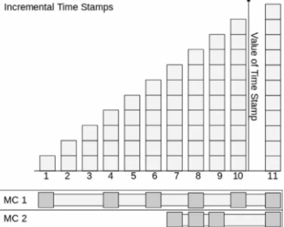
Scalable real-time classification of data streams with concept drift
Full text
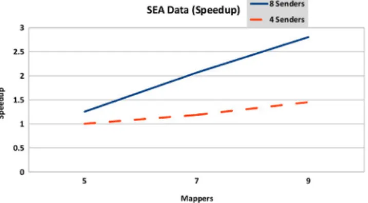
Figure

Related documents
20) Bachelor of Laws (Five Year Course) % Amended by Ordinance No.. 6 i) Environmental Studies shall be a compulsory subject for a previous year examination of the following
As marketing involves communication and delivering information to customers, all participants updated the information on their products or services through their
institutions to embrace new parameters and protocols. Finally, I will conclude with how COL has responded to the challenges of QA and provided support to Member States. But first
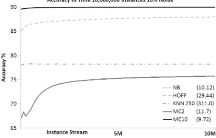
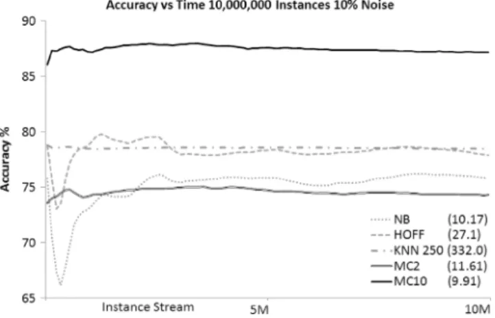
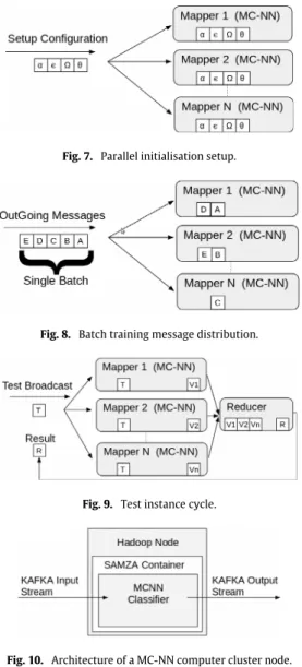
Hadoop performance is sensitive to network bandwidth. Replication or data movement across tiers during such net- work intensive phase may adversely affect the performance of the
Key words searched in the databases include director of nursing , DON, administration, nursing home , long-term care, turnover, intent to leave , intent to stay , role
Table 16 reports the results of the fixed-effect regressions with robust standard errors of next interval Tobin’s Q and ROA as they relate to the variable remuneration components
DIMMs, and hard disk drives, as opposed to their associated raw materials. This enables us to express the environmental impact of complex ensembles of diverse
