Interpretable Machine Learning

(1)

Master’s Thesis

Interpretable Machine Learning - An

Application Study Using the Munich

Rent Index

Julia Fried

Supervised by Prof. Dr. Bernd Bischl

Christoph Molnar Giuseppe Casalicchio

Ludwig Maximilians University Munich

Department of Statistics

(2)

Declaration of Authorship

I declare that I have authored this thesis independently, that I have not used other than the declared sources / resources, and that I have explicitly marked all material which has been quoted either literally or by content from the used sources.

Munich, October 15, 2018

(3)

Abstract

Machine learning can be used to model complex relationships. Usage of these algorithms is rare for business applications due to missing model interpretability and a resulting lack of trust in model decisions. The field of interpretable machine learning (IML) combines machine learning with tools that explain algorithmic decisions. Especially model-agnostic

methods are popular because they provide the ability to exchange the underlying machine learning models by maintaining the output form.

Model-agnostic methods are widely used in research, but less proven on practical examples and applications. This thesis analyses model-agnostic tools with regard to their global and local explainability. The methods are validated using a practical example, the estimation of the Munich rent index 2017. In order to explain global decisions of the machine learn-ing model, the Morris method and average marginal effects are compared, whereby average marginal effects prove to be more informative for the Munich rent index. Local decisions concern a specific observation and in this thesis LIME and Shapley values are analysed. Shapley values are more useful due to the underlying implementation and are chosen in this IML application study. The IML methods are implemented in an interactive dashboard to analyze algorithmic decisions and predict outcomes for instances.

In addition, the IML approach is compared with the “original” Munich rent index 2017, which is based on interpretable models. The question, whether the IML approach can be used to estimate the Munich rent index, is answered. As a result model-agnostic methods provide explanations for machine learning models and this work shows that the Munich rent index can be estimated with the IML approach. Model-agnostic interpretable machine learning offers enormous advantages because the underlying models are interchangeable and complex patterns in data can be explained globally and locally. Due to the state of de-velopment of the used IML methods, this thesis is experimental and requires further tests of interpretable machine learning in practical examples. Future research and improvement of the R packages will make interpretable machine learning a powerful tool and drive the commitment of machine learning in business applications.

(4)

List of Figures

1 Representation of nature . . . 1

2 Data modeling culture . . . 1

3 Algorithmic modeling culture . . . 2

4 Smooth functions in the MRI 2017 . . . 6

5 Feature importance plot . . . 17

6 PDPs for numeric and categorical features . . . 18

7 User specific values for local rent estimation . . . 19

8 Intuition behind LIME . . . 20

9 LIME plot . . . 21

10 Shapley plot . . . 22

11 AMEs in the global effects table . . . 24

12 PDPs in the global effects table . . . 25

13 Input value forms in the IML dashboard . . . 25

14 Results for local rent prediction . . . 25

15 Shapley value explanations . . . 26

16 Comparison categories for GAM vs. IML . . . 27

17 Splines vs. PDPs for living area . . . 33

18 Splines vs. PDPs for construction year . . . 33

19 Global effects I . . . 40

20 Global effects II . . . 41

21 Global effects III . . . 41

22 Input form for local effects . . . 42

23 Local rent estimation . . . 42

24 Shapley values for local explanations . . . 43

(7)

List of Tables

1 GAM formula abbreviations . . . 6

2 Surcharges and deductions of the MRI 2017 . . . 7

3 XGBoost tuning . . . 11

4 Random forest tuning . . . 11

5 SVM tuning . . . 11

6 Benchmark of GAM (*) and ML models regarding MSE and MAE. . . 12

7 AMEs partial derivative approximation . . . 14

8 Example of Morris method for four variables. . . 15

9 Example for different coding possibilities during AME calculation. . . 17

10 GAM coefficients vs. AME I . . . 31

11 GAM coefficients vs. AME II . . . 32

12 Used R packages . . . 44

(8)

Abbreviations

Abbreviation Meaning

AM Algorithmic modeling AME Average marginal effects CV Cross validation

DM Data modeling

GAM General additive models IML Interpretable machine learning

LIME Local interpretable model-agnostic explanations MAE Mean absolute error

ML Machine learning MRI Munich rent index MSE Mean squared error Rent / sqm Net rent per square meter OAT One-step-at-a-time

OLS Ordinary least squares PD Partial dependence PDP Partial dependence plots SVM Support vector machines XGBoost eXtreme Gradient Boosting

(9)

1. Potential of Interpretable Machine Learning

1

Potential of Interpretable Machine Learning

The following chapters give an introduction to different data modeling approaches and mo-tivate the use of interpretable machine learning (IML).

1.1

Challenges of Data-driven Decisions

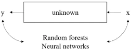
The use of data is essential for the management of successful businesses and for well-grounded decisions (Bose, 2009). Advanced analytics in particular offers the toolbox for data-driven decisions (Barton and Court, 2012). The goal of advanced analytics is to predict future events or to extract information from data. Both objectives intend to model a target variable y

from input variables x, with an unknown relationship, as shown in figure 1.

Figure 1: Symbolic representation of unknown relationship between input variables

x and target y.

The modeling of this nature can be done with various algorithms. The selection of a par-ticular algorithm depends on various factors, such as the complexity of the task, but also on the statistical culture to which the programmer belongs (Breiman et al., 2001). In the statistical world there are mainly two cultures: the “data modeling” (DM) culture and the “algorithmic modeling” (AM) culture, which define the approach how data is analysed. It also determines how the model output can be explained. The first group - the DM culture - assumes a stochastic data model inside the black box, where possible solutions are shown in figure 2.

The other group - the AM culture, often referred to as machine learning (ML) - treats the inside as a black box and thus as unknown. Instead of assuming a data model, the approach relies on finding an algorithm that predicts y based on input data x with best possible performance. Figure 3 shows some examples of possible algorithms (Breiman et al., 2001). The difference between the two approaches is that the DM culture concentrates on assuming a data model before starting the algorithmic process, and the AM culture does not need prior model assumptions, but selects algorithms based on their predictive accuracy. The first one has the advantage that a lot of structuring takes place before the real modeling

(10)

Figure 3: Examples for algorithms used by the algorithmic modeling culture.

process starts and thus the model itself can be simpler. These prior assumptions lead to more interpretable models, whereby interpretability in this case is “the degree to which an observer can understand the cause of a decision” (Biran and Cotton, 2017). Users are able to follow the decision path of the algorithm and explain the given results.

ML models have the advantage of flexibility and predictive accuracy, but come with a lack of model interpretability. This means that users do not understand the underlying logic of how the algorithm generates outputs. This leads to a lack of trust in business applications because the output of a model is not easy to explain. Subsequently, the results lead to a reduced acceptance of machine learning implementations as described by Barton and Court (2012).

In summary, it follows that interpretable models lack predictive accuracy and can not depict nature if patterns in the data are too complex for simple models. In contrast, flexible black box models are not interpretable and are less accepted by business users. Ideally, both goals - predictive accuracy and interpretability - are met. The research field of IML combine both goals, where various IML tools can explain model outputs. An interesting approach is the area of model-agnostic methods. These kind of methods extract ex-post explanations from the black box model and therefore allow the programmer to implement any algorithm and still interpret the model in the same way (Ribeiro et al., 2016a).

1.2

Motivation

Although there are different model-agnostic tools, practical examples are rare. Therefore, this master’s thesis aims to implement model-agnostic IML methods for a real use case.

To illustrate IML, the modeling process is applied to the Munich rent index (MRI) 2017. This case illustrates the tenant market in Munich and predicts appropriate rents for several apartment characteristics. The problem is actually solved with an interpretable regression algorithm in which all influencing factors can be precisely determined. The DM approach allows a comparison with other approaches and is one reason why this example is chosen.

(11)

Other intents are the data set itself, housing variables, such as the size of the housing or the year of construction, are easy to understand.

This master’s thesis analyses whether it is possible to use the MRI with machine learning models in combination with IML methods as an explanation and identifies opportunities and risks associated with the AM culture approach. Further motivation of this work is to compare several IML tools on the MRI and to identify suitable methods for concrete problems. The advantages and disadvantages associated with different methods are also validated.

1.3

Outline

This thesis is structured as follows: Chapter 2 explains the MRI and its model results. It addition, it defines an appropriate output for the IML alternative. Chapter 3 presents suitable machine learning algorithms for the named example and provides information about the selected black box model. In chapter 4 IML is introduced in detail and suitable tools for the rent index problem and their evaluation are shown. Additionally, changes that are made to the final IML methods are explained. Chapter 5 gives an overview of the result dashboard from the IML approach, which is discussed in chapter 6. The thesis concludes with a summary and an outlook in chapter 7.

(12)

2. Introduction to the Munich Rent Index

2

Introduction to the Munich Rent Index

This chapter provides more in-depth information about the MRI and explains its modeling process. The results of the model are explained and alternatives to the current calculation are provided.

2.1

Rent Indices as a Controlling Instrument of Renters Markets

This thesis uses the MRI as a case study for IML. One reason for the creation of the rent index is the exorbitant demand for affordable living spaces in German metropolises and the resulting extremely high rents (Windmann and Kauermann, 2017a). Rent indexes represent the local rent level on a broad information basis and have legal consequences if they meet the requirements for “qualified rent indexes”. These requirements are defined in§558 d BGB and determine that a rent index is legally binding if it has been created using recognized scientific methods and accepted by the township or representatives of landlord and tenants. In addition, a qualified rent index must be adapted to market changes every two years and re-created after four years (Bundesinstitut fuer Bau, 2014). The MRI is published by the city of Munich and provides a qualified rent index that establishes legal restrictions on rent increases and allows tenants to check whether they are paying reasonable rents in Munich (Windmann and Kauermann, 2017a).

In order to create the MRI, a representative data basis must be collected. This represents a random sample of all apartment types with their features in Munich. The sample is anal-ysed statistically in order to obtain a rent index and determines the influence of apartment characteristics on prices. Qualified rent indexes can be represented via “table rent indexes” or “regressions methods”. To generate table rent indexes, the housing market is represented by combinations of dwelling values (e.g. size under 40 sqm., simple apartment location) (Bundesinstitut fuer Bau, 2014), but the MRI is created using regressions methods. This has two advantages: On the one hand complex patterns can be illustrated, on the other hand the sample size can be much smaller than with table rent indexes. The latter almost requires a census, which is hardly feasible in Munich, in order to be able to produce a trustworthy rent index (Windmann and Kauermann, 2017b).

2.2

Statistical Background of the Munich Rent Index Calculation

As introduced in chapter 2.1, the MRI is created using regression methods. In this chapter, the requirements for the data set are discussed on the one hand, and the used regression

(13)

method of the MRI 2017 is analysed on the other hand.

Due to legal regulations, as described in §558 d BGB, not all available apartments in Mu-nich are included into the sample during the data collection process. For example, only flats where the rent has changed within the last four years, either due to rent increases or new rentals, are included. Another example of excluded dwellings are furnished or subleased ones. Flats that are eligible within the scope of the MRI are selected with a random sample. The data of these flats are collected via a questionnaire from landlords and renters. The interviewees answer questions about their apartment (e.g. size of flat, hot water supply or floor covering), the building (e.g. number of levels or type of building) and its location (like infrastructure or proximity to the center). A total of 577 different variables were collected for the MRI 2017 to explain prices of housing. Answers that had an extremely low occurrence, such as the absence of a bathroom or basement apartments, were deleted. In the MRI 2017, 3,222 questionnaires were collected. After the exclusion of 68 statistically meaningless obser-vations, 3,154 observations remained for statistical modeling (Windmann and Kauermann, 2017b). Even if 577 variables are available, not all are included to model the MRI 2017. A total of 21 variables is used, where the selection of the final features was determined via the significance tests and the AIC criteria (Akaike, 1974).

A specific regression method - generalized additive models (GAM) - is used to statistically model the target variable “net rent per square meter” (rent / sqm) (Windmann and Kauer-mann, 2017b). In this case the simple linear regression formulaY =β0+β1X (James et al.,

2013) is re-formulated into the GAM formula (StatSoft, 2006):

Y =g X

i

fi(Xi)

. (1)

fi are smooth functions of covariates, which allows a flexible specification of the dependence between the response variable and the covariates (Wood, 2003).

In the case of the MRI 2017 the general GAM formula is adapted to the rent index ques-tion. The GAM function for the MRI 2017 is formulated in equation 2 (Windmann and Kauermann, 2017b), where all abbreviations are explained in table 1.

rent / sqm =β0+f(L) +g(C) +β1X1 +β2X2+· · ·+ε. (2) f(L) and g(C) are smooth functions, where P

β0+f(L) +g(C) describes the average rent

(14)

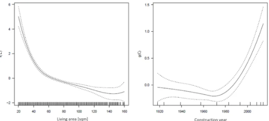
Figure 4: Estimated smooth functions for living area ˆf(L) and construction year ˆ

g(C) in the MRI 2017

Parameter Explanation L Living area [sqm]

C Construction year in which the building was constructed

X1, X2, . . . Further rent influencing factors like location of the flat, flooring or

hot water supply

Table 1: Abbreviations used in the GAM formula 2 for the MRI 2017.

2.3

Global and Local Effects for the Munich Rent Index 2017

The estimation of the MRI 2017 is a two-step weightedordinary least squares(OLS) method. The reason to have a two-step estimation procedure lays in a possible variance heteroscedas-ticity of the error term. First, an unweighted OLS is used to estimate rent/sqmˆ and squared residuals are determined to calculate the weights wi = 1/E(ri2). In a second step, the weighted OLS method is used to determine the MRI. The estimate of the base rent

P

β0+f(L) +g(C) is 11.23 EUR / sqm, where the smooth functions are plotted in figure 4.

The base rent depends on the living area and construction year and can be extracted from table 2 in Windmann and Kauermann (2017a) for specific apartments.

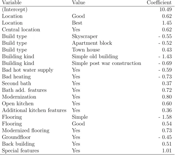
In addition to the base rent surcharges and deductions - further coefficients of the regression model - are necessary to predict the rent and are shown in table 2.

(15)

Variable Value Coefficient

(Intercept) 10.49

Location Good 0.62

Location Best 1.45

Central location Yes 0.62

Build type Skyscraper - 0.55

Build type Apartment block - 0.52

Build type Town house 0.43

Building kind Simple old building - 1.43 Building kind Simple post war construction - 0.69

Bad hot water supply Yes - 0.59

Bad heating Yes - 0.73

Second bath Yes 0.37

Bath add. features Yes 0.72

Modernization Yes 0.80

Open kitchen Yes 0.60

Additional kitchen features Yes 0.36

Flooring Simple - 1.58

Flooring Good 0.54

Modernized flooring Yes 0.73

Groundfloor Yes - 0.45

Back building Yes 0.51

Special features Yes 1.01

(16)

These results can be used on the one hand for a global interpretation according to table 2 and on the other hand to for the calculation of the estimated rent / sqm for a single apartment. The original implementation of the latter one can be found online1_.

2.4

Alternatives to the Current Rent Index Calculation

This chapter sets quantifiable objectives for an alternative MRI implementation. As ex-plained in chapter 1.1 there are two modeling cultures, where the current MRI implementa-tion is represented by the DM culture. In order to achieve the goals of predictive accuracy and interpretability, the AM approach in combination with IML (IML) is implemented. For similar results as the interpretable approach delivers, explainable results have to be created. This includes on the one hand a “coefficient”-like table (compare table 2), in which the algorithmic decisions are explained. On the other hand, it must be possible to predict rents for certain apartments and the output must be locally explainable.

To fulfill the goals from chapter 2.4, a new MRI estimation procedure were set up. It is intended to produce comparable results as in the GAM implementation, but using the AM approach. The IML process includes the following steps:

• Usage of the MRI data set,

• Selection of several, suitable ML algorithms and hyperparameter tuning,

• Benchmarking of results and usage of the best performance model,

• Identification and choice of suitable IML tools,

• Generation of an interpretable explanation for the best model with comparable results as the GAM model produces.

In order to formulate the last two points concretely global and local explanations are gen-erated. Global insights are a “coefficient”-like table, where the presented results should provide one effect per feature value to allow users to understand the relationships between the individual variables and the model explanation. The local explanation can be compared to the online calculator, presented in chapter 2.3. Additionally local decisions should be explained with IML tools.

(17)

3. Use of Machine Learning as an Alternative Approach

3

Use of Machine Learning as an Alternative Approach

In this chapter the ML part of the process (see 2.4) is explained in more detail. This includes the handling of the input data set, the selection of suitable ML algorithms and benchmarking of all models.

3.1

Modifications of the Input Data Set

The analysis of the input data describes the variables and their characteristics. As described in chapter 2.2, 577 raw variables were collected, but due to the variable selection based on significance tests and AIC criteria (Windmann and Kauermann, 2017b), 21 variables were included in the GAM model. The final variables can be taken from table 2, column “vari-able”. In the ML based approach, the same features are considered for two reasons: First, data protection reasons do not allow the use of all variables and the second reason is based on a better comparability of the GAM model and the IML approach.

The GAM model provides a global explanation and allows rent estimation for a specific apartment. The latter one is done using an online calculator and uses combinations of variables instead of the provided raw variables. In order to create consistency, the variable names are unified. Newly created is “residential situation”, which contains the original variables “location” and “centralized location”. The reason for this decision is the need for a combined feature in the online calculator to estimate the rent of an apartment. Users can only determine the residential situation on the basis of a specific city map2. Therefore the combined variable is used. Another change is made to the variables that contain information about the flooring. The original input data has separate variables, such as “good floor” [yes/ no] or “simple floor” [yes/ no]. These are summarized in the online calculator. Therefore, this thesis uses “flooring” as input variable.

3.2

Selection of Suitable ML Algorithms

To find the best algorithm for the rent index task, several algorithms were used and their performance compared. Based on algorithm classes presented in ML books from Friedman et al. (2001) and James et al. (2013) the following methods were used:

• Boosting,

• Random forests,

2_{Munich city map}

(18)

• Support vector machines (SVM) and

• Linear regression.

The first three algorithms are classical ML algorithms, the latter were chosen to analyze the performance of the MRI 2017 using a simple method for comparison purposes. The mean absolute error (MAE) and themean squared error (MSE) were used to measure the quality of the models and to select the best one. To ensure a fair measurement, all algorithms are validated with a 10-fold cross validation (CV). To further increase the performance, the hyperparameters of the ML models were tuned by performing random search with 200 it-erations. In order to measure the performance correctly, nested resampling was used. The selection of hyperparameters and their ranges is a manual process for which no standard procedure exists. In this thesis provided parameter configurations from the mlrHyperopt

package (Richter, 2017) are used. To be able to compare the different methods the R package

mlr3 were used. Below more information about the specific algorithms is given.

Boosting

The idea of boosting is the combination of weak classifiers into a powerful committee (Fried-man et al., 2001) and is strongly implemented in the tree-based XGBoost (eXtreme Gradient Boosting) algorithm. This method is used in the mlr learner regr.xgboost, which is se-lected to estimate the MRI 2017 with a boosting model.

The MRI data set contains a variety of factorial variables that can not be easily used for the XGBoost method. In practice, the input data set is edited to contain multiple numeric

dummy features4 _{that contain the same information as the categorical features.}

In case of the MRI modeling, the original variables are retained to enable a learner pre-sentation of global and local effects. Therefore, changes are made to the original XGBoost implementation so that dummy features are created within the algorithm for modeling pur-poses, but the output remains in the form of the original input data.

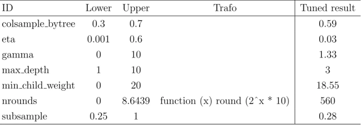
Since the XGBoost method does not provide good results on its own due to the large number of available parameters, tuning is essential. Table 3 shows the selected parameters and final hyperparameter settings.

3_mlr_{R package -}_{https://github.com/mlr-org/mlr}

4_{Dummy features are partitioned categorical features that contain the value 0 or 1 to show if a specific}

(19)

ID Lower Upper Trafo Tuned result

colsample bytree 0.3 0.7 0.59

eta 0.001 0.6 0.03

gamma 0 10 1.33

max depth 1 10 3

min child weight 0 20 18.55

nrounds 0 8.6439 function (x) round (2ˆx * 10) 560

subsample 0.25 1 0.28

Table 3: Tuning range and results for XGBoost on the MRI 2017 data set.

Random Forest

In the random forest algorithm, a number of decision trees are build on bootstrapped train-ing samples. Splits in a decision tree are based on a random sample ofmout ofppredictors. This process is known as decorrelation of trees and makes the result more reliable (James et al., 2013).

To build a random forest the mlrlearnerregr.randomForest is selected and table 4 shows the chosen hyperparameters and their results after tuning.

ID Lower Upper Tuned result

mtry 1 17 5

nodesize 1 10 9

Table 4: Tuning range and results for random forest on the MRI 2017 data set.

Support vector machines

SVMs have been historically developed for classification problems and separates two classes with a linear classifier and a maximum safety margin between the classes. For regression SMVs work vice versa: A functionf(x) with a safety margin is placed around the real func-tion.

Table 5 shows the tuned hyperparameters and their results, where regr.ksvm were used as learner.

ID Lower Upper Trafo Tuned result C −5 10 function (x) 2ˆx 26262.76 sigma −15 15 function (x) 2ˆx 0.000145252

(20)

Linear regression

To compare the tuned ML algorithms with a simple linear regression, the learner regr.lm

is used to build this model. In the next chapter the benchmark of all methods is described.

3.3

Usage of the Best Performance Model

The selection of the final model is based on MSE and MAE and additionally all results are compared with the performance of the GAM model (chapter 2.3). The GAM modeling process in the MRI did not include a CV based performance measurement. Therefore, the original GAM model is recalculated with CV to be comparable to the ML models. Table 6 shows the ML and GAM (*) models and their performance measurements.

MSE MAE XGBoost 4.63 1.62 GAM (*) 4.67 1.63 Random forest 4.70 1.62 SVM 4.73 1.63 LM 4.87 1.67

Table 6: Benchmark of GAM (*) and ML models regarding MSE and MAE.

The performance of the XGBoost model regarding MSE and MAE works best and this method is selected as final model.

(21)

4. Interpretable Machine Learning as Explanation for Black Box Models

4

Interpretable Machine Learning as Explanation for

Black Box Models

The following chapters describe model-agnostic IML methods that are suitable to explain the output of the MRI. The used methods are divided into global and local tools to achieve the goal of describing the overall model output and to understand the decisions made for one apartment.

4.1

Tools to Analyse Global Effects for the Munich Rent Index

In order to fulfill the goal of global explanations as described in chapter 2.4, the decisions of the ML algorithm must be explained. In detail, global means that the influence of all features is described together. In the sense of “global IML” different model-agnostic tools are avail-able. With regard to the the goal - to obtain a table with “coefficient” -like explanations for a regression task - two methods are analysed in detail: Average marginal effects (AME) and the Morris method. Furthermore, the selected “coefficient”-like effects are supplemented by variable feature importance and partial dependence plots (PDP) to provide further insights.

4.1.1 Average Marginal Effects

AMEs are the average influence of one variable as mean of the marginal effects over all observations and were designed for regression analysis (Best and Wolf, 2012). In a first step, marginal effects are determined for each observed value of X. Marginal effects can be calculated using partial derivatives and communicate the rate at whichy changes at a given point in covariates space with respect to one covariate dimension and holding all covariate values constant. In regression terms the marginal effect of one variable xj is the slope of the regression surface.

In common AME implementations (Leeper, 2017; Casalicchio, 2018) numerical derivatives are approximated with:

f0(x) = lim ε→0

f(x+ε)−f(x)

ε , (3)

where small steps ε in x are taken and ˆy is calculated at each point. An improvement to this simple difference method is the symmetric difference approach:

f0(x) = lim ε→0

f(x+ε)−f(x−ε)

2ε , (4)

(22)

the results are averaged to a single quantity per feature (Leeper, 2017).

In the approaches from Leeper (2017) and Best and Wolf (2012) AMEs can only be estimated for numerical features. The improvement by Casalicchio (2018) makes it possible to handle other data types, like factor variables. For factor variables, each characteristic is handled separately to obtain its own AME per feature characteristic. Therefore, in a first step, the different factor levels are separated for one feature xj. The variable xj is changed to keep one feature level only and predictions are made for the new data set, like shown in table 7. All predictions are averaged to one quantity and the described procedure is repeated until all averaged predictions are available per feature level. To obtain AMEs per feature characteristic, each characteristic is dummy coded, where the prediction of a feature characteristic is compared with a reference category, resulting in AMEs per feature characteristic.

xj all covariables prediction 0 original values prediction 1 0 original values prediction 2

.. .

0 original values prediction n

Table 7: Usage of R’s prediction() with a modified data set to approximate partial derivatives for factor variables.

The average marginal effects provide an intuition how much a certain variable (characteristic) increases or decreases the prediction of the target variable. In the case of the MRI the target variable is rent / sqm, for example 9.50 EUR / sqm for a specific apartment. For a variable characteristic the AME can be −0.50 EUR / sqm. This means that the rent / sqm is decreased by −0.50 EUR / sqm.

4.1.2 Morris’ Elementary Effects Screening Method

The Morris method is part of the scope of global sensitivity analysis and determines which inputs have important effects on an output (Morris, 1991). The Morris method is based on a so-called one-step-at-a-time (OAT) design, in which an input parameter xi is changed at each run and the model change is evaluated (Campolongo et al., 2005). With this method the input can be classified into three groups: variables with negligible effects, with linear effects that have no interaction and inputs with non-linear and/ or interaction effects. For screening techniques, which include the Morris method, the input space for each variable is discretized and several OAT designs are realized. The repetition of OATs helps to estimate

(23)

elementary effects for each input from which global effects can be derived. The elementary effect E_j(i) of the j −th variable is defined as (Iooss and Lemaˆıtre, 2015):

E_j(i) = f(X

(i)_{+ ∆}_e

j)−f(X(i))

∆ . (5)

(i) in this case describes thei−th repetitionrof the OAT design, whereris usually between 4 and 10 due to Saltelli et al. (2004). ∆ is a pre determined multiple of _n₋1₁ and ej is a vector of the canonical base.

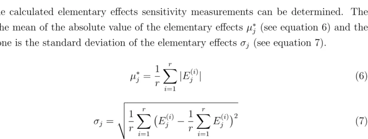
From the calculated elementary effects sensitivity measurements can be determined. The first is the mean of the absolute value of the elementary effects µ∗_j (see equation 6) and the second one is the standard deviation of the elementary effects σj (see equation 7).

µ∗_j = 1 r r X i=1 |E_j(i)| (6) σj = v u u t 1 r r X i=1 E_j(i)− 1 r r X i=1 E_j(i)2 (7)

µ∗_j measures the influence of variablej on the output and high values ofµ∗_j indicate that the input variable has an important influence on the output. σj provides information whether the input variable has interaction effects with other variables. Larger values indicate fewer linear features or interaction effects.

Table 8 shows an example for the MRI. The most important variables are selected, whereµ∗

provides a ranking for the features andσprovides information about linearity and interaction effects.

Variable Value mu sigma

Additional kitchen features 0 1.95 1.79 Flooring Good floor 1.93 0.56 Flooring Simple floor 1.14 0.39 Build type Apartment block 0.76 0.12

Table 8: Example of Morris method for four variables.

4.1.3 Usage of Average Marginal Effects as Final Method

In order to decide which of the methods is used in the MRI implementation, the advantages and disadvantages of both methods are compared. An advantage of the Morris method is

(24)

the affordable computation time, since the model only needs to be evaluated once for each run, which is linear in the number of model factors. Another advantage is the provision of a second indicator σ, which provides information about linearity and interaction effects by default. An important disadvantage is the sparse documentation of the Morris method for implementation purposes. Provided test examples are not suitable for an intuitive under-standing of the Morris method. Furthermore, the Morris results provide an intuition about feature importance, but no indicator how the target variable is influenced by one feature characteristic. To achieve a measurement that provides information about increase or de-crease in EUR / sqm the Morris method need to be adapted manually.

AMEs do provide effects per feature characteristic in EUR / sqm and additionally provide a simple interpretation and an intuitive way to describe relationships (Leeper, 2017). As explained in chapter 4.1.1, partial derivatives are required to explain global effects. In the case of the AME, a numerical approximation of the first derivative at point x is calculated via epsilon difference. When using tree-based methods this leads to problems if the step length ε is set too small.

As this thesis uses the tree-based XGBoost algorithm, the AME method must be adapted by setting an appropriate step length. The selection of ε is done semi-automatically by changing the step length and measuring the AME as output. If all features, where the PDP values differs in the continuous spectrum, have valid AMEs the step length is set.

Due to the simple interpretability and provision of effects for all features, the AME method is implemented in the MRI, where the results of the AME implementation are presented in chapter 5. Since the MRI data set contains a lot of factor variables, the AME process is analysed more closely for this type of variable: AMEs provide one effect per feature char-acteristic, and for categorical variables, the features are split by category. Each effect is provided per category. In the used R package ame (Casalicchio, 2018), the categorical fea-tures are dummy coded using a randomly selected category as reference category. In the case of the MRI, this coding makes the interpretation of AMEs more complicated. For example forresidential situation it is difficult for the user to derive effects from the reference category to another one. For this reason, the original coding is changed to effect coding. In this case, all effects are calculated to the mean effect instead of a reference category. The difference is shown in table 9.

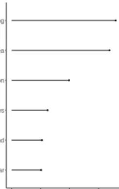
To provide additional information about the features, thefeature importance of each variable is considered. This measurement provides a quantity of importance for each variable and

(25)

Effect coded Dummy coded Average (light blue) -0.88

Good (yellow) -0.33 0.55 Best (light red) 0.42 1.31 Central average (dark blue) -0.49 0.39 Central good (orange) 0.41 1.29 Central best (dark red) 0.86 1.74

Table 9: Example for different coding possibilities during AME calculation.

describes how much a model relies on a specific feature (Breiman, 2001). It is calculated in the following manner: First, an error measurement eorg( ˆf) = L(Y,fˆ(X)) is calculated, for example, the MAE for regression problems. Next, each individual variable value Xj is permuted in a loop and in each loop the error measure is recalculated (eperm( ˆf)). The proportion of both errors is the feature importance for the selected variable (Fisher et al., 2018):

F Ij =

eperm( ˆf)

eorg( ˆf)

(8) Unimportant features are equal to one, because the model does not rely on this variable during prediction and therefore the error eperm( ˆf) does not change. An example for feature importance is plotted in figure 5.

In case of the MRI, MAEs are used to measure the error and, additionally, the number of shuffles is set to 20 to provide stable results.

● ● ● ● ● ● Construction year Building kind Additional kitchen features Residential situation Living area Flooring 1.00 1.05 1.10 1.15 Feature Importance F eature

Figure 5: Example for Feature importance, where the six most important features are visualized.

The AME method has the disadvantage that information is lost because all information is compressed to a single key figure. For example, nonlinear connections can not be displayed

(26)

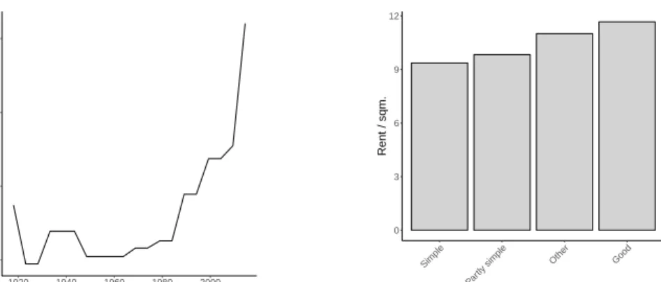
(Best and Wolf, 2012). To obtain the information of nonlinear connections, the single quan-tity is extended by PDPs. These plots are useful when the influence of one input variable is plotted on the output f(x) (Friedman, 2001). The partial dependence of f on the selected input variable xS is:

fS(xS) = EXC[f(xS, XC)] =

Z

f(xS, xC)dP(xC), (9)

where fS is the expectation of f over themarginal distribution of all variables xC excluding the variable of interest xS. To obtain PDPs in practice the average over the training data

Xi, i= 1, . . . , n with fixedxS is taken (Zhao and Hastie, 2017):

¯ fS(xS) = 1 n n X i=1 f(xS, XiC). (10)

The presentation of PDPs can be visualized with bar plots for categorical variables and as a line plots for numeric features. In the given example (figure 6), the rent / sqm increases if the apartment is in a building with a newer construction year and the rent also increases if the flooring in the flat is better.

11.0 11.5 12.0 12.5 1920 1940 1960 1980 2000 Construction year Rent / sqm. 0 3 6 9 12 Simple Par tly simple Other Good Flooring Rent / sqm.

Figure 6: Example for PDPs, where line plots visualize numeric features and barplots presents factor variables.

4.2

Tools to Analyse Local Effects for the Munich Rent Index

In order to be able to explain the estimated rent of a single apartment, different settings need to be considered. First, a user must be able to specify the feature values for a particular apartment, second, the underlying model must estimates the rent and third, the result must be explainable. The latter becomes more important for highly complex data patterns. If there is a strong non-linear connection within the data, it is useful to check the variable influ-ences on local level (Ribeiro et al., 2016b). Two methods are considered: Local interpretable model-agnostic explanations (LIME) and Shapley values.

(27)

4.2.1 Specification of Individual Feature Values

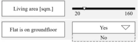
In order to estimate local effects, an observation of the data set is selected or a new obser-vation can be defined by a user. To allow users to estimate the rent for one apartment, the latter option is analysed. According to the GAM based MRI the range of possible input values is fixed to the underlying data set. Figure 7 shows possible ranges for living area and ground floor.

Figure 7: Symbolic insertion of user specific values for local rent estimation for the MRI 2017.

It must be taken into account how missing values, such as the absence of a value for “living area”, are handled. It is possible that the user may skip unknown entries or alternatively must enter all values. The options are

• Unknown values are replaced by suitable alternatives (mean/ median),

• A new model is estimated without the unknown features,

• The predicted rent is given as an interval to consider missing values or

• Missing values are not allowed.

The first option would use an alternative value, such as the mean value. It is possible that the input of this automatically calculated indicator strongly influences the output of the model and distorts the model. It is possible to exclude features and recalculation a new model, but on the one hand, is computationally intensive and on the other hand, compari-son between different apartments is more complex due to different models. The third option uses prediction intervals to overcome missing values and is not a standard procedure. To be able to use this option, further development is required to develop this solution. To be comparable with the original MRI online calculator5, the fourth option is chosen: Missing values are not allowed and the user must set all values before the rent is estimated.

Another point to consider is the order of input variables. In case of the MRI, the variables are ordered according to their feature importance, which is the same measurement as in chapter 4.1.3. The arrangement is inspired by best practices for creating web forms (Puri,

(28)

2012; Jarrett and Gaffney, 2009) and allows the user to fill in all required information in a simple and intuitive way.

Once it has been ensured that all necessary entries are made, the rent can be estimated and explained. In the next chapters, local interpretation methods are discussed.

4.2.2 Local Interpretable Model-agnostic Explanations

LIME is a local explanation method that is able to explain a single observation. For this method, local surrogate models are fitted, which are interpretable models like decision trees or linear models. These interpretable models enable the user to understand decisions of the black box model.

The LIME explanation defines the following optimization problem:

ξ(x) = arg min g∈G

L(f, g, πx) + Ω(g). (11)

L(f, g, πx) measures how unfaithfully the selected surrogate modelg approximates the black

box model f. LIME explains a specific observation and measures how close the selected instance of interest z and x are with the proximity measure πx. To keep surrogate models interpretable, a complexity measurement Ω(g) is minimized. To ensure that this method is model-agnostic, which means thatf stays a black box,L(f, g, πx) needs to be approximated. Therefore samples around x0 are chosen randomly, which lead to a new observation of inter-estz0. For this instance a prediction is generated and equation 11 is optimized. By this, the surrogate model explains the local observation (Ribeiro et al., 2016b).

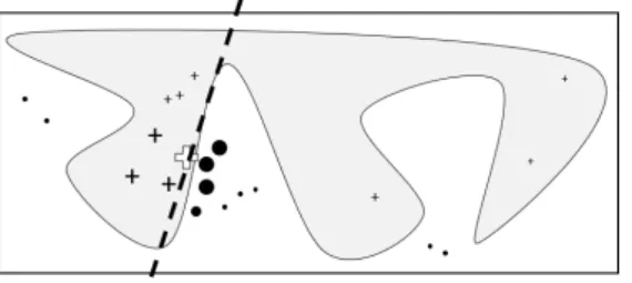
Figure 8: Intuition behind LIME to describe the local explanation (Ribeiro et al., 2016b)

Figure 8 visualizes the idea of LIME. Shown is a decision function in white/ grey and the selected observation of interest (white cross). The aim is to explain the black box model for this instance. Therefore new sample observations are drawn from the neighborhood of the target observation and predictions for these samples are generated with the black box

(29)

model. The closer the sample is to z, the higher the weight πx. By optimizing equation 11 the interpretable model separates two classes (crosses and dots) and provides a local explanation for the observation of interestz.

Figure 9 shows the LIME explanation for one example. An observation is selected from the MRI data set and six features are explained by LIME. It becomes clear that “building kind = other” has a positive effect on the rent, while the other features have negative effects. In particular, “simple floor” causes a rent reduction by about 1.20 EUR / sqm for this observation.

Flooring = Simple floor Additional kitchen features = 0 Residential situation = Average (light blue) Open kitchen = Other kitchen type Special features = Not available Building kind = Other

−1.0 −0.5 0.0 0.5

Effect

F

eature v

alue

Figure 9: Example for LIME plot with six explained feature values.

4.2.3 Shapley Values

The goal of the Shapley value method, proposed by Strumbelj and Kononenko (Strumbelj and Kononenko, 2014), is to explain the contribution of input features for an individual observation.

The contribution is expressed by a quantity which denotes the influence of a feature value. The quantity can be positive, negative or zero. A positive one increases the prediction for the observation, a negative one decreases it and a zero feature value has no impact.

The method works by changing the inputs and observing the outputs, to meet the require-ment of being model-agnostic. To handle computational power, a subset of M instances is sampled from the data set and the Shapley value φij (established by Shapley (Shapley, 1988)) is approximated by Monte-Carlo sampling (Strumbelj and Kononenko, 2014):

ˆ φij = 1 M M X m=1 ˆ f(x∗+j) ˆf(x∗−j), (12)

where the prediction ˆf(x∗+j_{) for} _x

i. has randomly exchanged feature values from a random data point x, except for feature value xij. For ˆf(x∗−j) the procedure is similar with the

(30)

difference that xij is included in the sample from x (Lundberg and Lee, 2016).

The interpretation of the Shapley value φij is the contribution of the feature value xij to the prediction for the selected observation compared to the average prediction for the data set. Figure 10 shows an extract of the calculated Shapley values for the MRI data set as an example. Shown is the same observation as in the LIME example (see figure 9). Six features and their specific values are visualized in the plot. The selection is based on the absolute highest Shapley values for this example. It is shown that “building kind = other” has a positive effect on the rent and the other five variables have a negative trend. As in the LIME example, a simple flooring has the greatest negative effect, for this observation a simple floor contributes −1.60 EUR / sqm to the compared to the average prediction.

Flooring = Simple floor Residential situation = Average (light blue) Additional kitchen features = 0 Construction year = 5 Modernized flooring = No modernized floor Building kind = Other

−1.5 −1.0 −0.5 0.0

Phi

F

eature v

alue

Figure 10: Example for Shapley plot with six explained feature values.

4.2.4 Usage of Shapley Values as Final Method

The decision which method - LIME or Shapley values - is implemented in the MRI tool is based on the comparison of advantages and disadvantages of both methods. The use of lin-ear models to explain the outcome allows an easy interpretation for LIME. This is because effects can be interpreted as regression coefficients. On the other hand LIME does have key drawbacks: First LIME relies on distance measurements to determine the neighborhood of the instance of interest, which is a disadvantage in a high dimensional space (“curse of dimensionality” (Keogh and Mueen, 2011)), and also there exist no standard procedure for choosing weight for πx. Related is the disadvantage of kernel width definition. The kernel width defines the neighborhood and it is not obvious which width to choose. Furthermore, the user must manually select k features. In the case of the MRI the goal is to explain the complete prediction, therefore all features should be by default explainable, which is not proposed in LIME. Another disadvantage is the usage of surrogate models. If the underlying relationship between the variables is too complex, even for the local instance, LIME can not

(31)

explain the decisions that are made by the machine learning model.

Compared to LIME, the interpretation of Shapley values is more complex because all effects are given in the relation to the average prediction. Another drawback is the selection of the number of samples. The more samples are chosen, the higher the required computational power. This limits the programmer to manually select a manageable amount of samples, which is not a standard procedure. The Shapley method has a major advantage in the cal-culation process: First, this method is based on solid theory, based on mathematical axioms from game theory (Shapley, 1988). It is ensured that the Shapley method fairly distributes the difference between the actual prediction and the average prediction among the feature values of the instance. For these reasons, the Shapley value method is used for the local effects analysis.

Due to the use of Shapley values in this thesis, the sample size must be determined, which is done via experiments: For one observation the difference between actual and average pre-diction is compared to the averaged sum of Shapley values for different sample sizes. Ideally the averaged sum of Shapley values converges to the difference between actual and average prediction. This steps are repeated for different observations and the plots (see Appendix D) are compared. As a result there does not exist the right sample size, but different exper-iments showed that a sample size of 150 is a good trade-off between computational power and trust able results.

(32)

5. Result Presentation with Shiny Dashboard

5

Result Presentation with Shiny Dashboard

The results for global and local effects in the MRI application study are published for users. Therefore, a shiny dashboard6 _{was created, where on the one hand the global effects are}

shown for the ML model and on the other hand an user can interactively estimate a rent for an apartment. The dashboard has two benefits: First, an online tool is created for the IML MRI and these results can be easily compared with the original rent index calculation. The second advantage is having a showcase for IML and its usage possibilities.

The app is published underhttps://juliafried.shinyapps.io/MunichRentIndex/and is structured in an introduction page, the global effects table and an interactive rent estimation for one flat. In the following, examples for the latter two pages are given.

5.1

Global Effects Table

The global effects table provides AMEs, PDPs and feature importance for all feature values. Figure 11 shows an extract of the lowest and highest effects.

Figure 11: Highest and lowest AMEs with their corresponding feature values.

The table is ordered by “AME” (third column: Effect), which shows the increase or decrease in the target variable rent / sqm, if a feature characteristic (first and second column: Feature

and Value) is present. For example increases the occurrence of a good flooring (last element in the table) the rent / sqm for an apartment by around 1.10 EUR compared to the average.

As described in chapter 4.1 the AME provides a single quantity per feature characteristic, which can be too compressed for non-linear connections. Therefore the PD curves are added in the fourth column (PDP). For categorical features the the PDP shows the predicted target variable “rent / sqm” with the selected feature characteristic in pink. PDPs for numerical

(33)

variables show the predicted rent in a continuous curve with highlighted spikes in pink. An example for PD curves for categorical and numerical features is shown in figure 12.

Figure 12: Excerpt of PDPs for numeric and categorical variables of the global effects table.

5.2

Local Effects Explanation

The “rent index calculator“ page allows to estimate the rent for a single apartment and explains the results locally with Shapley values. In order to be able to estimate the rent, all input values must be set first. Depending on the feature type, an user must select the feature with a slider (numeric values) or by dropdown (categorical variables), as shown in figure 13. To make the input process as simple as possible, all input fields are preset with mean values for numeric features and with the mode for categorical features.

Figure 13: Excerpt from the input values form to request user input for a specific apartment.

Figure 14: Predicted rent for a specific apartment.

After querying all variable values, the rent for the given flat is estimated. Figure 14 shows the corresponding result. Beneath the estimated results a visualized local explanation is given,

(34)

as shown in figure 15. A slider filter is provided so that the user can concentrate on the most important (highest and lowest) values. All Shapley values are provided in numerical form, too, if the user prefers to view the explanations in text form.

(35)

6. Discussion of Results

6

Discussion of Results

To be able to quantify the differences between the DM and AM approach and therefore synonymic the GAM model and the IML method, both solutions are compared. In the latter chapter the limitations and chances of used IML methods are discussed.

6.1

Comparison of the Two Approaches

To compare the two approaches theimplementation process and theoutput is analysed. Both categories are split to sub-categories and are discussed on a lower level, as shown in figure 16.

Figure 16: Visualization of the comparison categories to analyse GAM and IML approaches.

6.1.1 Implementation Process

The implementation process is similar for the DM and the AM approaches: First, the data set must be prepared, which includes, for example, handling of missing values or feature se-lection. In the next step, one or more models are fitted to the data set and the performance is measured. After the pure modeling, the results are analysed and interpreted. But even if the process is similar on the surface, the details differ. The following subcategories show relevant differences.

Feature selection. The variable selection is done via significance tests and additionally ac-cording to the AIC criteria (see 3.1). The same data set is used to model the alternative approach, but it is important to address how features are selected in the DM and AM com-munities in practice. The first selects the variables before starting the modeling process, for example through significance tests. In the ML culture feature selection can also take place before the model is fitted, but it is also possible to include this step into the modeling process. This has the advantage that features in the pipeline are automatically selected and manual work can be avoided. Another perspective relevant to this paragraph is one reason

(36)

why feature selection is performed. Due to the desire of simple, interpretable models, to avoid overfitting (Windmann and Kauermann, 2017b) and also to include the most rele-vant variables only, the DM community uses the variable reduction to receive a manageable model. The AM community has no need to select input variables. In many cases, this step can be omitted and powerful models are achieved. In the case of the MRI the situation is different. Since the user must fill in all variable values to estimate the rent for a flat (see chapter 4.2.1), it does not make sense to include all variables in the model.

Model choice. The GAM model is selected from expert knowledge and prior assumptions that can be made after manual analysis data patterns, which makes it possible to have a fairly simple model that fits well with the data, but requires manual thought and data anal-ysis before starting the modeling process begins. Especially in the case of the MRI, where the data patterns are complex, interaction effects and smooth functions (see 2.2) must be determined manually and lower the model interpretability. In contrast, ML pipelines enable a a semi-automated modeling process and provide the best model. Today, hyperparameter tuning requires manual work, but the development of automated parameters selection is well advanced, enabling an automated pipeline.

Runtime. Due to data set preparation and careful model selection the runtime for the GAM model is fast, which is not given for the chosen ML models. In case of the MRI data set, the GAM model delivers results in seconds and the comparison and tuning of ML models takes hours. Longer runtimes can be justified through hyperparameter tuning on the one hand and benchmarking of several models on the other hand. It is questionable how important runtimes are. Nowadays it is possible to rent fast servers for an affordable price and the ML comparison process can be done much faster.

Interchangeability. The MRI is redone every two years (see 2.1) and therefore it is impor-tant to build on a framework that can be reused. In the DM approach the model must be re-developed each time. Due to a similar task, the GAM model is recycled and adjusted in practice. The IML pipeline is an automated process, newly collected data can be integrated into the machinery and the IML output is preserved. Manual work is required for perfor-mance validation and potential hyperparameter changes. Besides the MRI task the provided IML pipeline including the dashboard (see chapter 5) can be used for any data and tasks due to an automated process and model-agnostic IML tools. This advantage is important because it allows the usage of one pipeline to solve multiple problems and explain various tasks with a dashboard.

(37)

6.1.2 Output

In the category “output” the performance and the interpretability are discussed. The output of the GAM model - the coefficients table - is compared to the IML approach.

Performance. Both, the DM and the AM approaches, have a high performance, where the performance table described in chapter 3.3 calculates the model quality as in the ML culture. With respect to performance, two different perspectives are analysed: First, the difference how the DM and AM community measure “goodness of fit”, and second, the specific indi-cators are compared. The DM and AM approaches differ during the model fitting process, they also differ in the determination of performance criteria. The quality of the GAM model is measured by internal criteria such as AIC or deviance, which can lead to unreliable and overly optimistic indicators. In the case of the MRI, the AIC is an important measurement, but the focus is less on performance measurement than on variable selection and output explanation. In contrast a ML model is trained and tested on different kind of data. During model testing an external performance criteria, such as MSE or MAE, is estimated. To ensure a well calculated indicator, CV is used. Due to the more reliable measurement of the ML modeling process, this approach is preferable.

As shown in 3.3, the quality of the GAM model in terms of MSE and MAE is very good. It is useful to further deepen the development of the MRI in order to discuss the goodness of fit of the GAM model. As described in chapter 3.1, the same variables are used for for estimating ML models as are used for the regression model. Possible is that the performance of the ML models improve with access to all input variables. Due to data security reasons, it is not possible to validate this hypothesis. Another reason that can influence a good GAM performance is inspired by the theory of the self-fulfilling prophecy by Merton (1948). It says that the prophecy or rather prediction is fulfilled due to indirect or direct causes. In the case of the MRI, two options are offered to positively influence the performance. First, the landlords are bound to the qualitative rent index (see 2.1) and thus future rents are influenced by the output of the GAM model. Second, the questionnaire to collect the input data is influenced by the GAM model, it is possible that variables that are not used to model the MRI for several years are excluded from the questionnaire and therefore influence the input data in favor of the GAM model.

Interpretability. The interpretation of linear regression models is simple due to the linear relationship between input and output. As output, a table with coefficients and confidence intervals is provided to analyse the effects of features on the target variable. In the case of the MRI, a more complex model is used to depict more complex patterns, like non-linear

(38)

relationships and interaction effects. The risk of misinterpretation is increased for the output of this more complex GAM model (Leeper, 2017). Another drawback is that variables that are modeled via splines are not be expressed in one number.

The intrinsic interpretability as provided for linear models is not given for ML models that are used to model the MRI. Therefore, additional tools must be used to explain the decisions of the black box. Compared to the DM approach AMEs, see chapter 4.1, are used to get a “coefficient”-like table as provided in the GAM model. After the creation of this table, the interpretability is intuitive, even for non-statisticians. Additionally further tools are imple-mented to increase model insights: PDPs and feature importance. PDPs provide information about the linearity of numeric variables and show the connections between different feature values for categorical variables. The feature importance method provides insights about the most relevant variables for the underlying algorithm. In addition to the global insights, local IML tools are applied to explain the model for single observations. The used Shapley values (see 4.2) visualize the feature values contribution to the final prediction, which allows users to get an overview of important effects at first glance. It allows users to understand the decisions, even if no further thoughts are given to the global model. Another advantage of IML is that the tools can be used with any model after the initial set up and do not require adaptions.

Comparison of global effects. In a first step, the GAM coefficients and global effects are compared. Table 10 and 11 shows the coefficients and AMEs of the variables.

(39)

Variable Value GAM Coefficients AME

(Intercept) 10.49 NA

Back building Yes 0.51 -0.25

Back building No NA 0.25

Bad heating Yes -0.73 -0.36

Bad heating No NA 0.36

Bad hot water supply Yes -0.59 -0.30

Bad hot water supply No NA 0.30

Build type Skyscraper -0.55 -0.28

Build type Apartment block -0.52 -0.37

Build type Town house 0.43 0.51

Build type Other NA 0.14

Building kind Simple old building -1.43 -0.62 Building kind Simple post war construction -0.69 -0.02

Building kind Other NA 0.64

Living area Range from 20 to 160 ∗2) _-0.03

Construction Year Range from 1918 to 2014 ∗2) _0.001

Flooring Simple -1.58 -1.10

Flooring Partly simple ∗1) _-0.64

Flooring Good 0.54 1.20

Flooring Other NA 0.54

Modernized flooring Yes 0.73 0.54

Modernized flooring No NA -0.54

Groundfloor Yes -0.45 -0.24

Groundfloor No NA 0.24

Modernization Yes 0.80 0.29

Modernization No NA -0.29

Table 10: Comparison of GAM coefficients and AMEs of the MRI (I/II)

∗1) _{Interaction effect with simple floor}

(40)

Variable Value GAM Coefficients AME

Add. kitchen features Yes 0.36 NA

Add. kitchen features 0 NA -0.77

Add. kitchen features 1 NA -0.17

Add. kitchen features 2 NA 0.49

Add. kitchen features 3 NA 0.45

Open kitchen Yes 0.6 0.25

Open kitchen No NA -0.25

Residential Situation Average NA -0.85 Residential Situation Central average NA -0.52

Residential Situation Good NA -0.36

Residential Situation Central good NA 0.42

Residential Situation Best NA 0.50

Residential Situation Central best NA 0.81

Location Good 0.62 NA

Location Best 1.45 NA

Central location Yes 0.62 NA

Second bath Yes 0.37 0.40

Second bath No NA -0.40

Bath add. feat Yes 0.72 0.39

Bath add. feat No NA -0.39

Special features Yes 1.01 0.40

Special features ... No ... NA -0.40 Table 11: Comparison of GAM coefficients and AMEs of the MRI (II/II)

Since the GAM model is dummy coded, the reference categories are marked with “NA”. The comparison between the different codings is possible though, for example if the apartment is located in a “back building”, the GAM coefficient is 0.51 EUR / sqm in relation to the reference category (apartment is not in back building). The corresponding AMEs are 0.25 and −0.25 EUR / sqm (in back building/ not in back building). The further comparison shows that the directions of all feature characteristics are the same for the DM and AM approach and that all values are close. Special cases are the location-related variables and living area/ construction year. The first case occurs due to a different data labeling. The coefficients-table contains “location” and “central location”, but is used as one variable in the online calculator. In this thesis the variables are combined to “residential situation” and therefore the results are less comparable. It turns out that for the combined variable

(41)

central good and (central) best locations have an positive influence on the rent / sqm. The GAM coefficients are positive if the location is good or best and a central location has an positive effect. The other special case are the spline modeled variables “living area” and “construction year”. In the DM approach these variables are not expressed in a coefficient, but the visualization in a plot is preferred. Figure 17 and figure 18 shows the splines vs. the PDPs of the corresponding variables to compare the trends: Larger apartments have a lower rent / sqm and the construction year influences the rent with an increasing trend, but also older buildings have more higher influence. This process causes an AME around 0, which is shown in table 10. 10 11 12 13 14 15 40 80 120 160 Living area Rent / sqm.

Figure 17: Splines of GAM model and PDPs for living area of MRI 2017

11.0 11.5 12.0 12.5 1920 1940 1960 1980 2000 Construction year Rent / sqm.

Figure 18: Splines of GAM model and PDPs for construction year of MRI 2017

6.2

Chances and Limitations of the IML Application Study

The challenges and opportunities of IML are discussed below. In particular, the use of methods in this thesis and their practical problems are compared to advantages of IML.

6.2.1 Practical Problems With Current Methods

Development of IML methods. The development of IML methods is new, where problems like missing documentation or mathematical checks occur. The used papers, for example the

(42)

LIME paper (Ribeiro et al., 2016b) was published in 2016 and the use of Shapley values for IML (Strumbelj and Kononenko, 2014) was suggested in 2014. In contrast the GAM paper (Hastie and Tibshirani, 1986) was published in 1986 and improved from there on. Regarding AMEs used in this thesis, no paper has been published so far, and as such the use of AME in this thesis is experimental. There is an AME paper for regression models from Leeper (2017) and AMEs have also been validated in the paper from Best and Wolf (2012), but the mentioned literature is not exactly what is implemented in the used ame R package. Since many IML methods are new and in an experimental phase, the underlying mathematical proofs are not given in every case. As explained in chapter 4.2.4, the comparison between LIME and Shapley values has opted for the Shapley method due to stable mathematical axioms which prove correctness of Shapley values.

R package implementation. R packages for IML methods used in this thesis are new, for example the ame package was released on GitHub in 2017. Also, the iml package that is used to produce PDPs, feature importance and Shapley value explanations was published on CRAN in March 2018. These new packages present several challenges: First, examples and tutorials explaining how to implement the provided methods are sparse. Second, the methods must be adjusted manually to achieve the MRI goals, and third, packages updates can affect the functionality of the dashboard.

Using the Morris method is quite complex due to a lack of explanation. The method is pro-vided by thesensitivitypackage, but only one example is given. The same problems occur with theamepackage, with the difference that the AME implementation is closely related to the mlrpackage, which is well documented. Practical problems with the AME method arise in this thesis because AMEs were developed for regression algorithms. This thesis uses tree-based methods, such as XGBoost, that require manual adaption of the step length within the package. The latter challenge faces package updates. New features can break the dash-board. An example is the creation of PDPs with the imlpackage. The implem