OpenBU http://open.bu.edu
Theses & Dissertations Boston University Theses & Dissertations
2016
Sequence queries on temporal
graphs
https://hdl.handle.net/2144/17056
GRADUATE SCHOOL OF ARTS AND SCIENCES
Dissertation
SEQUENCE QUERIES ON TEMPORAL GRAPHS
by
HAOHAN ZHU
B.E., Tsinghua University, 2007 M.E., Chinese Academy of Sciences, 2010
Submitted in partial fulfillment of the requirements for the degree of
Doctor of Philosophy 2016
First Reader
George Kollios, PhD
Professor of Computer Science
Second Reader
Evimaria Terzi, PhD
Associate Professor of Computer Science
Third Reader
Mark Crovella, PhD
HAOHAN ZHU
Boston University, Graduate School of Arts and Sciences, 2016 Major Professor: George Kollios, Professor of Computer Science
ABSTRACT
Graphs that evolve over time are called temporal graphs. They can be used to describe and represent real-world networks, including transportation networks, social networks, and communication networks, with higher fidelity and accuracy. However, research is still lim-ited on how to manage large scale temporal graphs and execute queries over these graphs efficiently and effectively. This thesis investigates the problems of temporal graph data management related to node and edge sequence queries. In temporal graphs, nodes and edges can evolve over time. Therefore, sequence queries on nodes and edges can be key com-ponents in managing temporal graphs. In this thesis, the node sequence query decomposes into two parts: graph node similarity and subsequence matching. For node similarity, this thesis proposes a modified tree edit distance that is metric and polynomially computable and has a natural, intuitive interpretation. Note that the proposed node similarity works even for inter-graph nodes and therefore can be used for graph de-anonymization, network transfer learning, and cross-network mining, among other tasks. The subsequence match-ing query proposed in this thesis is a framework that can be adopted to index generic sequence and time-series data, including trajectory data and even DNA sequences for sub-sequence retrieval. For edge sub-sequence queries, this thesis proposes an efficient storage and optimized indexing technique that allows for efficient retrieval of temporal subgraphs that satisfy certain temporal predicates.For this problem, this thesis develops a lightweight data management engine prototype that can support time-sensitive temporal graph analytics ef-ficiently even on a single PC.
1 Introduction 1
2 Node Sequence Query 6
3 Existing Node Similarity Measures 9
3.1 Node Similarity Applications . . . 9
3.2 Node Similarity . . . 10
3.3 Categories of Node Similarity . . . 11
3.4 Link Similarities . . . 12
3.4.1 Distance-based Similarity . . . 12
3.4.2 SimRank-based Similarity . . . 12
3.4.3 HITS-based Similarity . . . 14
3.4.4 Random Walk-based Similarity . . . 15
3.4.5 Sampling-based Similarity . . . 16
3.4.6 Link-based Similarity Conclusion . . . 16
3.5 Neighborhood Similarities . . . 17
3.5.1 Neighbor Set Similarity . . . 17
3.5.2 Neighbor Vector Similarity . . . 18
3.5.3 Feature-based Similarity . . . 18 3.5.4 Path-based Similarity . . . 20 3.5.5 Role-based Similarity . . . 20 3.5.6 Graphlets-based Similarity . . . 21 3.6 Discussion . . . 23 v
4.1 Introduction . . . 24
4.2 Related Work . . . 27
4.3 NED: Inter-Graph Node Similarity with Edit Distance . . . 28
4.3.1 K-Adjacent Tree . . . 28
4.3.2 NED . . . 29
4.3.3 NED in Directed Graphs . . . 30
4.4 TED*: Modified Tree Edit Distance . . . 31
4.4.1 Edit Operations in TED* . . . 32
4.5 TED* Computation . . . 33
4.5.1 Algorithmic Overview . . . 35
4.5.2 Node Padding . . . 35
4.5.3 Node Canonization . . . 36
4.5.4 Bipartite Graph Construction . . . 39
4.5.5 Bipartite Graph Matching . . . 40
4.5.6 Matching Cost Calculation . . . 41
4.5.7 Node Re-Canonization . . . 42 4.6 Correctness Proof . . . 43 4.7 Metric Proof . . . 44 4.7.1 Identity . . . 45 4.7.2 Triangular Inequality . . . 46 4.8 Isomorphism Computability . . . 48 4.9 Complexity Analysis . . . 51
4.10 Parameter K and Monotonicity . . . 51
4.11 TED*, TED and GED . . . 53
4.12 Weighted TED* . . . 54
4.13 Experiments . . . 57
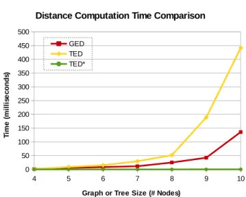
4.13.1 TED*, TED and GED Comparison . . . 58
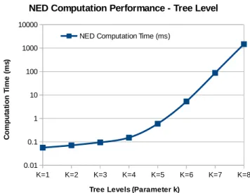
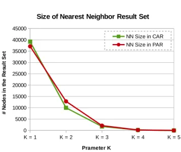
4.13.3 Analysis of Parameter k . . . 61
4.13.4 Query Comparison . . . 63
4.13.5 Case Study: De-anonymizing Graphs . . . 65
4.14 Conclusion . . . 66
4.15 NED for Graph Similarity . . . 67
5 A Generic Sequence Query Index: Reference Net 70 5.1 Reference Net Introduction . . . 70
5.2 Reference Net Related Work . . . 72
5.3 Reference Net Preliminaries . . . 74
5.3.1 Similar Subsequences . . . 75
5.3.2 Query Types . . . 76
5.3.3 Using Metric Properties for Pruning . . . 77
5.4 The Consistency Property . . . 77
5.5 Segmentation . . . 80
5.6 Indexing Using a Reference Net . . . 82
5.7 Algorithms for Reference Net . . . 86
5.7.1 Insertion . . . 86
5.7.2 Deletion . . . 87
5.7.3 Range Query . . . 88
5.8 Subsequence Matching . . . 88
5.9 Experiments . . . 91
5.9.1 Space Overhead of Reference Net . . . 93
5.9.2 Query Evaluation . . . 97
5.10 Reference Net Conclusions . . . 101
6 Edge Sequence Query: LiTe-Graph Engine 103 6.1 LiTe-Graph Introduction . . . 103
6.2.1 Temporal Graph Model . . . 105
6.2.2 Temporal Subgraph Query . . . 107
6.3 Storage Representation . . . 108
6.4 Index on Temporal Edges . . . 110
6.4.1 Temporal Indices . . . 110
6.4.2 Index on Temporal Edges . . . 111
6.4.3 Improved Index on Temporal Edges . . . 113
6.5 Time-Sensitive Analytics . . . 117
6.5.1 PageRank . . . 117
6.5.2 Temporal Shortest Path Finding . . . 118
6.5.3 Other Algorithms . . . 119
6.6 System Overview . . . 119
6.7 Real-World Temporal Graphs . . . 121
6.7.1 Temporal Graph Extraction . . . 121
6.7.2 Life Span Distribution . . . 122
6.8 Evaluation . . . 124
6.8.1 Experimental Settings . . . 124
6.8.2 Experiments . . . 124
6.9 LiTe-Graph Related Work . . . 134
6.10 LiTe-Graph Conclusion . . . 136
7 Conclusions 138
List of Journal Abbreviations 140
Bibliography 143
Curriculum Vitae of Haohan Zhu 153
3.1 Node Similarity Applicability Comparison . . . 22
4.1 Notation Summarization for TED* Algorithm . . . 34
4.2 NED Datasets Summary . . . 56
5.1 Computation Ratio of RN and CT for Proteins . . . 98
5.2 Computation Ratio of RN and CT for for Songs . . . 99
6.1 Lite-Graph Notation Summarization . . . 109
6.2 Temporal Index Comparison . . . 111
6.3 LiTe-Graph Datasets Summary . . . 122
3.1 An Example of Node Roles . . . 10
3.2 How similar betweenA and α ? . . . 19
4.1 K-Adjacent Tree . . . 29
4.2 TED* vs Tree Edit Distance . . . 32
4.3 Node Canonization . . . 37
4.4 Completed Weighted Bipartite Graph Construction . . . 41
4.5 Computation Time Comparison Among TED*, TED, and TED . . . 56
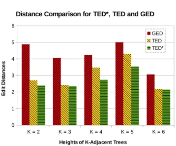
4.6 Distance Comparison Among TED*, TED, and TED . . . 57
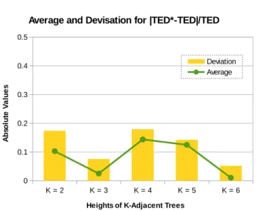
4.7 Distance Relative Error Between TED* and TED . . . 58
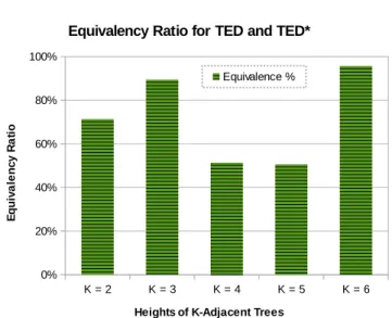
4.8 Equivalency Ratio Between TED* and TED . . . 59
4.9 TED* Computation Time . . . 60
4.10 NED Computation Time . . . 61
4.11 Nearest Neighbor Query vs Parameter k . . . 62
4.12 Top-l Ranking vs Parameter k . . . 63
4.13 Computation Time Among NED, HITS, and Feature . . . 64
4.14 NN Query Time of NED with VP-Tree . . . 65
4.15 De-Anonymize PGP Graph . . . 66
4.16 De-Anonymize DBLP Graph . . . 67
4.17 De-Anonymization with Different Permutation Ratio . . . 68
4.18 De-Anonymization with Different Top-kFindings . . . 69
5.1 An Example of Reference Net . . . 83
5.2 Difference between Net and Tree. . . 85 x
5.4 Distance Distribution for PROTEINS . . . 91
5.5 Distance Distribution for SONGS . . . 92
5.6 Distance Distribution for TRAJ . . . 92
5.7 Space Overhead forPROTEINS . . . 94
5.8 Space Overhead forSONGS . . . 95
5.9 Space Overhead forTRAJ . . . 96
5.10 Query Performance for PROTEINS. . . 97
5.11 Query Performance for SONGSin DFD Space . . . 98
5.12 Query Performance for SONGSin ERP Space . . . 99
5.13 Query Performance for TRAJ in ERP Space . . . 100
5.14 Query Performance for TRAJ in DFD Space . . . 100
5.15 Query Results for PROTEINS . . . 101
6.1 Temporal Graph and Temporal Edges . . . 106
6.2 Two Examples of Temporal Subgraphs . . . 108
6.3 LiTe-Graph Architecture . . . 121
6.4 Edge Life Span Distribution . . . 123
6.5 Edge Life Span Distribution Cont. . . 123
6.6 Temporal Graph Storage Space Comparison . . . 125
6.7 Covering Subgraph Query Time Comparison . . . 126
6.8 Persisting Subgraph Query Time Comparison . . . 127
6.9 Temporal Subgraph Query vs Query Ranges . . . 128
6.10 Temporal Subgraph Query vs Starting Positions . . . 129
6.11 Revisitings with Different Datasets for LiTe-Graph . . . 130
6.12 Revisitings with Multi-threads for LiTe-Graph . . . 131
6.13 LiTe-Graph Performance with Multi-threads . . . 132
6.14 LiTe-Graph System Parameter Analysis . . . 133
6.16 In-Memory LiTe-Graph . . . 135
BLAST . . . Basic Local Alignment Search Tool BWT . . . Burrows-Wheeler Transform CT . . . Cover Tree
DBLP . . . Computer Science Bibliography DFD . . . Discrete Fr´echet Distance DNA . . . Deoxyribonucleic Acid
DSD . . . Dense Snapshot-Delta Combination DTW . . . Dynamic Time Warping
EB . . . Edge Bitmap
ERP . . . Edit Distance with Real Penalty ES . . . Edge Stream
FPGA . . . Field-Programmable Gate Array GED . . . Graph Edit Distance
GPU . . . Graphics Processing Unit HITS . . . Hyperlink-Induced Topic Search IP . . . Internet Protocol
LiTe-GRAPH . . . Lightweight Temporal Graph Engine MVBT . . . Multi-Version B-Tree
NC . . . Node Centric
NED . . . Inter-Graph Node Similarity with Edit Distance NN . . . Nearest Neighbor
PGP . . . Pretty Good Privacy PPI . . . Protein-Protein Interaction RN . . . Reference Net
SNP . . . Strict Non-Deterministic Polynomial-Time SS . . . Snapshot Sequence
SSD . . . Sparse Snapshot-Delta Combination TED . . . Tree Edit Distance
TED* . . . Modified Tree Edit Distance VP-TREE . . . Vantage Point Tree
G(t) . . . A temporal graph
u(ts, te) . . . A node sequence
T(u, k) . . . k-adjacent tree of nodeu
Li(u) . . . ith-level of k-adjacent tree of nodeu C(n) . . . Canonization label of node n
x⊏y . . . Node x is a child of node y Pi . . . Padding cost for the level i Mi . . . Matching cost for the level i G2
i . . . Complete bipartite graph in the level i w(x, y) . . . Edge weight in G2i betweenx andy m(G2i) . . . Minimal cost for G2i matching
fi :fi(x) =y . . . Node mapping function forG2i matching Q . . . A query sequence with length|Q|
X . . . A database sequence with length|X|
SX . . . A subsequence of X SQ . . . A subsequence of Q
E(t) . . . Temporal graph in temporal edge set
Esub(t) . . . Temporal subgraph in temporal edge set T . . . Series of time stamps
e(u, v, ts, te) . . . A temporal edge
l=te−ts . . . Life span of a temporal edge
tx,ty . . . Thresholds for query conditions n . . . Number of edges
B . . . Bucket size
f(·) . . . Hashing function
bi . . . ith bucket for hashing table r . . . redundancy ratio
Introduction
In the era of Big Data, the management and analytics of graph and sequence (or time series) data is an essential topic, because not only can such data grow rapidly to extremely large sizes, but they are also important representations of data from many real-world applications. For example, graph data are used to organize social networks, biological protein-protein interaction (PPI) networks, transportation networks, and communication networks, among others. Meanwhile, sequence or times series data are used, for example, to represent DNA sequences, trajectories, songs, stock market statistics and many kinds of economic and financial information.
Much research has focused on graph data and sequence data management and ana-lytics. However, the fusion of graph data and sequence data has generated a new field, temporal graphs, for which research on efficient management and analytics is limited. Tem-poral graphs are a promising research area from which real-world applications will benefit tremendously. Therefore, this thesis focuses on sequence queries, which are fundamental to temporal graph management and analytics.
First, this thesis introduces some real-world applications of temporal graphs. As de-scribed above, collaboration, transportation, and communication networks can be format-ted into graphs. In real-life settings, those networks are not static and may evolve over time. For example, consider DBLP collaboration networks in which the nodes are authors. If two authors collaborate on a publication, an edge connects them. Every year, author collaborations on publications may change. Moreover, very few authors have exactly the same collaborators for two consecutive years. If we consider only the aggregated
collabo-rations for the whole time period in DBLP, which is a stack graph, it will be difficult to tell how authors’ collaborations evolve, and it also will not be accurate to compare two authors and judge whether they have similar collaboration patterns or not.
Another example comes from communication networks such as autonomous system networks in which the nodes are autonomous systems: if two systems communicate, an edge exists between them. Like the collaboration networks, in communication networks the autonomous system topologies vary from day to day. It is hard to find exactly the same topologies on two consecutive days. If we consider only the aggregated autonomous system topologies, it will be difficult to conduct analytics on them for designated periods, as in the case of computing centralities of autonomous systems for a certain period when system connections are stable.
According to the above instances, it is clear that temporal graphs differ significantly from static graphs because temporal information exists in graphs and is important in ana-lytics. Meanwhile, temporal information introduces difficulties in managing and analyzing temporal graphs. Notice that it is also hard to extend the management and analytics to classic temporal data for temporal graphs. The temporal graph is a special type of tem-poral data where each object on a specific timestamp is a graph, whereas classic temtem-poral data management and analytics usually deal with numeric values and character sets. Thus, managing and analyzing temporal graphs efficiently forms a novel domain and becomes a challenging task.
This thesis focuses on sequence queries on temporal graphs, namely node sequence and edge sequence queries. Such queries are unique and fundamental in temporal graph management and analytics. First, only in temporal graphs may nodes and edges evolve over time. Node sequences and edge sequences merely exist in temporal graphs. Second, node sequence queries can be used to find similar nodes or similar node behaviors. In different applications, nodes may represent different objects. In collaboration networks, similar nodes could mean similar authors, while in communication networks, similar nodes may stand for similar autonomous systems. Overall, node sequence queries can help
iden-tify similarities among network entities. Third, edge sequence queries are the most basic building blocks for finding temporal subgraphs, which are needed for time-sensitive ana-lytics on temporal graphs, such as computing centralities in autonomous system networks when the connections are stable or investigating connectivities in mobile networks when all connections are completed. Overall, edge sequence queries are key components in assisting time-sensitive analytics of temporal graphs.
In this thesis, the node sequence query decomposes into two building blocks: graph node similarity and generic subsequence query. Because the node sequence query detects similar node behaviors, it is essential to first define a similarity measure for a pair of nodes, then apply the sequence query to node sequences. For the node similarity, this thesis proposes a modified tree edit distance that is metric and polynomially computable and has a natural intuitive interpretation. Note that the proposed node similarity is a metric for inter-graph nodes and therefore can be used for graph de-anonymization, transferring learning across networks, and performing biometric pattern recognition, among other tasks. The generic subsequence query proposed in this thesis is a framework that can be adapted for indexing sequence and time-series data, including trajectory data and even DNA sequences for subsequence retrieval. On the other hand, for the edge sequence query, the edge sequence can be used to express evolving subgraphs that satisfy certain temporal predicates. For this problem, this thesis proposes and describes a lightweight data management engine prototype that can support time-sensitive temporal graph analytics efficiently even on a single PC.
To summarize, the contributions of this thesis are listed below:
• This thesis thoroughly investigates existing node similarity measurements and com-pares those measures based on applicabilities.
• This thesis proposes a novel inter-graph node metric based on edit distance (NED).
– Real-world graphs demonstrate that NED is efficient for nearest neighbor node query and top-k similar node ranking tasks.
– NED can achieve a higher precision in graph de-anonymization tasks.
• This thesis introduces a modified tree edit distance (TED*) that is both metric and polynomially computable on unordered, unlabeled trees.
– TED* is a good approximation to the original tree edit distance whose compu-tation on unordered unlabeled trees is NP-Complete.
• This thesis proposes a generic indexing framework for sequence and time series data that makes minimal assumptions about the underlying distance and thus can be applied to a large variety of distance functions.
– This thesis introduces the notion of Consistency as an important property for distance measures applied to sequences.
– This thesis proposes an efficient filtering algorithm that produces a shortlist of candidates by matching only O(|Q| · |X|) pairs of subsequences, whereas brute force would match O(|Q|2· |X|2) pairs of subsequences.
– This thesis introduces a generic indexing structure called Reference Net with linear space; range similarity queries can be further efficiently answered based on Reference Net.
– The generic indexing framework is empirically demonstrated to provide good performance with diverse metrics such as the Levenshtein distance for strings, and ERP and the discrete Fr´echet distance for time series.
• This thesis proposes a lightweight temporal graph management engine called LiTe-Graph.
– LiTe-Graph can efficiently manage large-scale temporal graphs (up to a billion edges) on a single PC.
– LiTe-Graph is space- and time-efficient (in milliseconds) for temporal subgraph queries.
– LiTe-Graph improves temporal hashing for faster temporal subgraph queries.
– LiTe-Graph is compatible with existing graph algorithms for time-sensitive an-alytics on temporal graphs.
– LiTe-Graph has been evaluated using many real-world temporal graphs from diverse applications.
The following thesis is organized as follows:
• Chapter 2 investigates the existing node similarity measurements with their applica-bilities.
• Chapter 3 briefly describes the node sequence query problem and splits it into two subroutines: inter-graph node similarity and generic sequence index.
• Chapter 4 proposes NED, a novel inter-graph node metric based on edit distance that uses a modified tree edit distance, TED*.
• Chapter 5 discusses a generic indexing framework with Reference Net. Combined with NED, the framework can answer node sequence queries efficiently.
• Chapter 6 introduces LiTe-Graph, a temporal graph engine that provides efficient edge sequence queries on temporal graphs.
Node Sequence Query
This chapter introduces the first query type, node sequence query, which it splits into two independent subroutines: inter-graph node similarity measurements and generic sub-sequence retrieval.
Firstly, the node sequence is defined formally. Let a temporal graphG(t) be a sequence of graph snapshots G(t) =< G1, G2, . . . , Gn >, where each graph snapshot Gi is a static
graph associated with a time stampti. Let T be the series of time stamps for the temporal
graph G(t). ThenT =< t1, t2, . . . , tn >. A snapshot can be represented as Gi = (Vi, Ei),
whereVi is the vertex set and Ei is the edge set at the time stampti.
Assume there is a nodeuexisting from time stamp tsto time stampte, which meansu
∈Vi,∀s≤i≤e. Then the node sequence ofu fromtsto tecan be represented asu(ts, te)
=< us, us+1, . . . , ue>.
The node sequence query problem is defined as:
Definition 1. For a given node sequence u(tus, tue), find the most similar node subsequence
v(tv
s, tve) in the temporal graph G(t).
Notice that, the time stamp tus may not be the same as tvs. Also, the time stamp tue
may not be the same as tv
e. Therefore, two node sequences may not have the same length
and may span different sets of snapshots in the temporal graph. Furthermore, nodeuand nodev may even belong to different temporal graphs. Therefore, the first problem derived from node sequence query is how to define the similarity between two node sequences, and the second problem is how to efficiently find the most similar subsequence.
Fortunately, there are many distance functions for sequences or time-series that can be used for measuring pairwise node sequences, such as dynamic time warping (DTW) distance, ERP distance, or discrete Fr´echet distance. However, if those distance functions are used, an underlying distance between pairwise objects in the sequences or time-series should be formalized. For example, if discrete Fr´echet distance is used to measure two tra-jectories, there should be an underlying distance for pairwise 2D locations (2-dimensional vectors), usually Euclidean distance. If ERP distance is used to measure the two songs, there should be another underlying distance for pairwise pitches (integer values), usually the Hamming distance. Therefore, when distance functions for node sequences are used, there should be an underlying distance to measure the pairwise nodes. Ideally, this un-derlying distance should be a metric and should be capable of handling a pair of nodes in different graphs.
Hence, to conduct the node sequence query, the first key step is to find an inter-graph node similarity measurement that is a metric. Chapter 3 first investigates all existing node similarity measurements; unfortunately, no existing measurement can satisfy the re-quirements for the node sequence query. However, Chapter 4 proposes a novel label-free inter-graph node similarity measurement that satisfies all metric properties.
Because many different distance functions can be used for comparing pairwise node sequences, the second key step is to design a generic subsequence indexing framework that can benefit a variety of distance functions for sequences and time-series. Chapter 5 introduces a generic subsequence indexing method that works for diverse metrics such as the Levenshtein distance for strings, ERP, and the discrete Fr´echet distance for time series. Overall, the node sequence query can be split into different tasks as described in Chapter 3, 4, and 5. Combining the inter-graph node similarity in Chapter 4 with the generic subsequence indexing method in Chapter 5 can solve the node sequence query effectively and efficiently.
Chapter 3 provides a comprehensive study of node similarity measurements and com-pares and analyzes existing node similarity measurements according to their applicabilities.
The analysis demonstrates a lack of node similarity measurements that can measure pair-wise nodes in different graphs without additional information other than the topological structures and at the same time satisfy the metric properties. As a measurement, sat-isfying the metric properties is important and valuable because a metric measurement is compatible with many metric indexing techniques for accelerating query speed.
Thus, Chapter 4 proposes a novel inter-graph node metric based on edit distance called NED that satisfies all metric properties. NED introduces a new modified tree edit distance (TED*). The computation of classic tree edit distance on unlabeled, unordered trees is NP-Complete. However, TED* is a metric that is also polynomially computable on unlabeled, unordered trees. According to the empirical study, TED* provides a good approximation to the classic tree edit distance. As an inter-graph node similarity, NED can be used for graph transfer learning, graph de-anonymization, and many other stand-alone applications. Finally, Chapter 5 proposes a generic subsequence indexing method that can be com-bined with any metric measure in diverse domains, such as sequences, time series, or strings. Consider a node sequence as a sequence of topological structures: when the node similarity is metric, it is easy to adopt any sequence or time-series distance function for the node sequence. Therefore, using the reference net introduced in the generic subsequence indexing method can enable efficient retrieval of the node subsequence. Notice that, the generic subsequence indexing method is not only designed for node sequence query. It can be even used to any kind of sequence and time-series data which has a very large variety of applications.
Existing Node Similarity Measures
3.1 Node Similarity Applications
Graph, as a commonly used representation for describing the real-world data, has received a lot of attentions from many different areas. Graph is utilized to organize data in com-munication networks, social networks, and biological networks, to name a few.
Node is the basic component of graphs. In communication networks, the nodes are machines. In social networks, the nodes are people. While in biological networks, the nodes are genes and proteins. Measuring the similarity between two nodes is an essential task and also a fundamental building block for graph analysis.
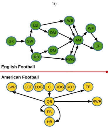
Figure 3.1, shows two graphs: english football positions and american football positions. In these two graphs, the nodes are the player positions and the edges indicate the passing paths in general. Consider the following question: How similar (in terms of functionalities) between a sweeper (SW) and an attacking midfielder (AM) in an english football team? How similar (in terms of roles) between an attacking midfielder (AM) in an english football team and a quarterback (QB) in an american football team? To answer such kind of questions, a measurement to describe the similarity for pairwise nodes in graph structures is needed.
Similarly in social network graphs, people may want to know how relative of one person to the other one in a social network. Such measure may indicate how fast the information can be propagated from one person to the other one. Also people may want to know for a given person in her/his own social network, whether there is another person in a different
Figure 3.1: An Example of Node Roles
social network has the similar impact or role. For example, which current english football player has the most similar impact in the soccer social network as “Tom Brady” in the current american football players’ social network.
All of above applications require a measurement to describe how similar of two nodes in graph structures. However, different applications consider different aspects of the nodes. Therefore, there exists many different node similarities which measure a pair of nodes according to different criteria. In this chapter, the existing node similarity measurements are briefly summarized and categorized.
3.2 Node Similarity
Given two nodes: nodeu in graphGa(Va, Ea) and nodevin graphGb(Vb, Eb) respectively,
where u ∈ Va and v ∈ Vb. Let the node similarity between a pair of nodes be s(u, v). In
the counterpart, let the node distance between a pair of nodes be d(u, v) which describes the node dissimilarity. Indeed, both node similarity and node distance can answer the
question: How similar between nodeu and nodev?
In this chapter, only the node similarity measurements that take the linkage information from graphs into account are included. Such node similarity measurements sometimes are called as structure-based similarities. In the opposite way, there is another type of content-based comparisons which only consider the attribute or property information of nodes. For example, a sweeper (SW) and an attacking midfielder (AM) may be compared based on their heights, weights, speeds and durations. But none of these properties is related to the linkage information in a graph. Therefore, such kind of node similarity measurements is not considered in this chapter.
Notice that, the graph Ga(Va, Ea) and graph Gb(Vb, Eb) may be the same graph which
indicates that two nodes to be compared should be in the same graph. There is a com-parative study [77] which compare a number of link-based similarities between two nodes in the same graph. In this chapter, all kinds of node similarities are considered, no matter the pair of nodes belong to the same graph or belong to two different graphs.
3.3 Categories of Node Similarity
In [77], the node similarity measurements are categorized into two major classes: similarity for homogeneous graphs and similarity for heterogeneous graphs. While in [57], there is another categorization which classifies the node similarity measurements based on the functionalities into two parts: node roles and node proximities.
This chapter mainly splits the existing node similarity measurements into two groups based on the structural information they use for the comparisons. If a node similarity mea-surement may use the linkage information from the whole graph to compare two nodes, it is called as global-link-based similarity or link-based similarity for short. As a counter-part, if a node similarity measurement merely use the linkage information from the local neighborhood subgraphs to compare two nodes, it is called as local-neighborhood-based similarity or neighborhood-based similarity for short.
All the measurements mentioned in [77] belong to the linked-based similarity measure-ments in this chapter. However, this chapter also discusses the linked-based similarity measurements which can deal with two nodes in different graphs. Compared to [57], node proximities are usually measured by link-based similarities. Whereas, node roles can be measured by both link-based similarities and neighborhood-based similarities.
3.4 Link Similarities
In this section, the link-based similarities are split into five different sub-classes: shortest path distance-based similarity, SimRank-based similarity, HITS algorithm-based similarity, random walk algorithm-based similarity and sampling graph-based similarity.
3.4.1 Distance-based Similarity
The very basic idea to measure the similarity between two nodes is to use shortest path distance or minimal weighted distance between two nodes. In [56], several distance-based similarity measurements are enumerated called graph theoretic distances. However, such straightforward distances are efficient but ignore information from related paths between two nodes. Distance-based similarity can be used for special cases of graphs, for example, uncertain graphs. Potamias et al. [96] proposes a distance function for a pair of nodes in uncertain graphs which is kind of distance-based similarity for special graphs.
3.4.2 SimRank-based Similarity
Among a huge amount of link-based similarities, SimRank [45] is the most popular mea-surement which says two objects are similar if they are related to similar objects. Here “related” means connecting by edges. The SimRank is defined ass(u, v) for a pair of nodes
u and v below: sk+1(u, v) = C |I(u)||I(v)| |I(u)| X |I(v)| X sk(I(u), I(v)) (3.1)
where I(u) and I(v) are the sets of in-neighbors of u and v respectively and C is a decay factor.
Tremendous research work follows SimRank and improves it from different aspects. They compose a big family of SimRank-based similarities. Several papers improve the computation speed for SimRank. Thek-iteration time complexity of the original algorithm of SimRank is O(kn2d2), where n is number of nodes in graph G and d is the average
incoming degree of nodes. Lizorkin et al. [78] improves the computational complexity of SimRank from O(kn4) to O(kn3) in the worst case. Yu et al. [132] further speeds up the
computation of SimRank toO(kd′n2), whered′ is typically much smaller than the average incoming degree of nodes. Power-SimRank [14] makes use of the power-law distribution of similarity scores to reduce iterations for some vertices. Li et al. [72] propose to compute SimRank between a specified pair of node which is much faster than computing all-pairwise SimRank.
Moreover, there are many papers [64, 30, 60] which investigate top-k SimRank com-putation for a single source node. The linearization method proposed by Kusumoto et al. [60] can linearly compute approximated SimRank for a single source. Yu et al. [136] even improve the quality of approximated SimRank.
There are also some variants of SimRank proposed to address the drawbacks of the original SimRank. For example, P-Rank [143] jointly combines both in-link and out-link in the computation. PSimRank [28], Simrank++ [3] and MatchSim [75] try to solve a common problem in SimRank: the similarity will decrease if number of common neighbors increases. SimRank* [134] investigates the problem of zero similarity which is due to the asymmetric path between a pair of nodes. RoleSim [46] considers a problem in SimRank that if two nodes are automorphic, the similarity should be maximal which is not true in SimRank. Although MatchSim and RoleSim try to solve different problem in SimRank, both of them consider not only global transitivity information but also local neighborhood information. Different from SimRank which considers all pairwise neighbors in each iteration, MatchSim and RoleSim try to pick one neighborhood matching in each iteration.
Some other work on SimRank includes: non-iterative solution for SimRank proposed by Li et al. [70], paralleled algorithm to deal with SimRank by He et al. [41] and partial-pairs SimRank computation by Yu et al. [135].
In the application level, Sun et al. [112], Zheng et al. [144] and Tao et al. [116] utilize SimRank for similarity joining. While Yin et al. [131] adopt SimRank for clustering. Xi et al. [126] introduce a SimFusion which consider heterogeneous data sources but share the similar idea with SimRank. Moreover, recently, there are some work [90, 133] focuses on SimRank computation for evolving or dynamic graphs.
SimRank-based similarities compose a hug family of node similarities which are very popular to measure the proximity between a pair of nodes in one graph.
3.4.3 HITS-based Similarity
Beside the SimRank-based node similarity measurements, there is another type of node similarities which are based on HITS algorithm [53] introduced by Kleinberg. Blondel et al. [12] propose a measure of similarity between a pair of vertices in two directed graphs. The similarity matrix is defined in an iterative function:
Sk+1 =BSkAT +BTSkA (3.2)
where A and B are two adjacency matrices of two graphs. Let A be ann ×n matrix and let B be anm ×m matrix. While S is an m× nsimilarity matrix. The entry (u, v) of S is the similarity value between the node u in graphA and the nodev in graph B.
Initially, the similarity values of all pair-wise nodes in the similarity matrix are set to 1. By iteratively updating the similarity matrix, the similarity matrix finally oscillates between two limits, w.r.t even limit and odd limit.
Clearly, if n and m are large, the node similarity matrix is not feasible to compute. There are some papers [137, 89] which consider local neighborhood subgraphs of two nodes instead of the whole graphs. Such methods can reduce the size of matrices to be multiplied.
However, number of iterations for the convergence may still be large in the computation. The HITS-based similarities also use linkage information to compare nodes. Notice that, although HITS-based similarity tries to compare two nodes in two different graphs, the absolute similarity values in the similarity matrix are not comparable in general. It only tells that among the nodes from another graph, which one will be more similar to a given node.
Be more specific, assume there are three nodes: u in graph A,v in graph B and w in graphC. Even if the similarity value between uand v in the matrix from graph A andB
may be larger than the similarity value between u andw in the matrix from graphA and
C, it does not mean the node uis more similar to node v than node w.
3.4.4 Random Walk-based Similarity
Besides the family of SimRank-based similarities and HITS-based similarities, there is another kind of similarities which also utilize the adjacency matrix and transitivity infor-mation to measure the similarity between two nodes.
Random walk with restart [92, 118] is a typical solution which can provide a good relevance score between two nodes in a weighted graph as shown in Equation (3). Koutra et al. [26] adopt fast belief propagation to compute node affinities which represent the similarity between pairwise nodes in the same graph in their algorithm DeltaCon. Fast belief propagation is identical to personalized random walk with restart under specific conditions.
~ri=cW˜ ~ri+ (1−c)~ei (3.3)
Personalized PageRank [40] is another solution which generates query-specific impor-tance scores. The topic-sensitive PageRank is able to deliver the imporimpor-tance ranking for a given query node.
et al. [65] proposes a vertex similarity in networks. Their method finds that two vertices are similar if their immediate neighbors in the network are themselves similar. Symeonidis and Tiakas [114] transform the adjacency matrix into a similarity matrix which is based on the degree of each node. Then by computing the products of the shortest paths between each pair of nodes, the extended matrix represents the similarities between pairwise nodes in the same graph. Line et al. [74] proposes a PageSim which computes similarity by using PageRank scores.
The random walk-based similarities usually compare two nodes int the same graph, since two nodes should be reachable by links. The exception is similarity flooding [84]. The similarity flooding can calculate pairwise node similarities between two different graphs, since the similarity flooding generates one propagation graph from two target graphs. The propagation graph generation relies on edge labels which are required to be matched from two target graphs.
3.4.5 Sampling-based Similarity
There are some other link-based similarities which consider a subset of edges from the original graphs which are called as sampling-based similarity in this chapter.
Zhang et al. [140] utilizes random path to provably and quickly estimate the similarity between two nodes. The similarity describes how likely two nodes appear on a same path after randomly sampling several paths with a given length.
Panigrahy et al. [93] proposes a node affinity. In the node affinity, for a given probability threshold, the maximum fraction of edges that can be deleted randomly from the graph without disconnecting two reachable nodes is defined as the affinity between those two reachable nodes.
3.4.6 Link-based Similarity Conclusion
Link-based node similarities compare two nodes based on the graph transitivity and infor-mation propagation to represent how close two nodes are. Those measurements may use
the linkage information from the whole graph. All SimRank-based similarities, most ran-dom walk-based similarities (except similarity flooding) and all sampling-based similarities compare two nodes in the same connected graph since only if two nodes are reachable, there exists the proximity between them. The HITS-based node similarities and similarity flooding can compare two nodes in two different graphs, because these methods generate a virtual single graph based on the linkage information from two graphs. In most cases, the link-based node similarities consider the topological information only which means there is no extra information needed for those measurements. Similarity flooding, otherwise, needs edge labels in the comparison.
3.5 Neighborhood Similarities
In this section, the neighborhood-based similarities are split into six different sub-classes: neighbor set based similarity, neighbor vector based similarity, feature vector based simi-larity, path based simisimi-larity, role based similarity and graphlets based similarity.
3.5.1 Neighbor Set Similarity
The neighbor set similarity measure two nodes by comparing the neighbors of two nodes. The two neighbor sets are usually compared by using set comparison methods such as: Jaccard coefficient, Sørensen–Dice coefficient, Ochiai coefficient and so on.
In [79, 110, 127], the instant neighbors of two nodes are compared to represent the node similarity. In SCAN[127], the structural similarity of two nodes is defined as:
σ(u, v) = p|Γ(u)∩Γ(v)|
|Γ(u)||Γ(v)| (3.4) where Γ(u) and Γ(v) are the instant neighbor sets of nodeu and v respectively. Usually such similarities work for two nodes in the same connected graph and the compared nodes should be close to each other. Otherwise, if two nodes do not share any common neighbor, the similarity will be always 0.
3.5.2 Neighbor Vector Similarity
Lu et al. [80] extend the comparison between instant neighbor sets tok-hop neighbor sets. Firstly, two authority value vectors of k-hop neighbors are computed by using the HITS algorithm. The authority value vectors are inn-dimensions wheren is number of nodes in the union set of two k-hop neighbor sets. Then the node similarity is computed by using the cosine distance between two authority value vectors.
Khan et al. [49] propose a neighborhood-based similarity measurement (Ness) which also compares two nodes based on their k-hop neighbors. Firstly Ness constructs two neighborhood vectors of nodes u and v according to the neighbors’ labels and distances. The neighborhood vector of u is denoted by R(u) = {hl, A(u, l)i}, where l is a neighbor label andA(u, l) represents the strength of labell.
A(u, l) = h X i=1 αi X d(u,v)=i I(l∈L(v)) (3.5)
where α is a constant propagation factor between 0 and 1. Then the cost function or distance function between two nodesu andv is defined as:
CN(u, v) =
X
l∈RQ(v)
M(AQ(v, l), Af(u, l)) (3.6)
whereM is a positive difference function.
Similarly, in NeMa [50], the node similarity is defined by using the same neighborhood vector, but the cost function is normalized which can provide a better result for graph matching problem.
3.5.3 Feature-based Similarity
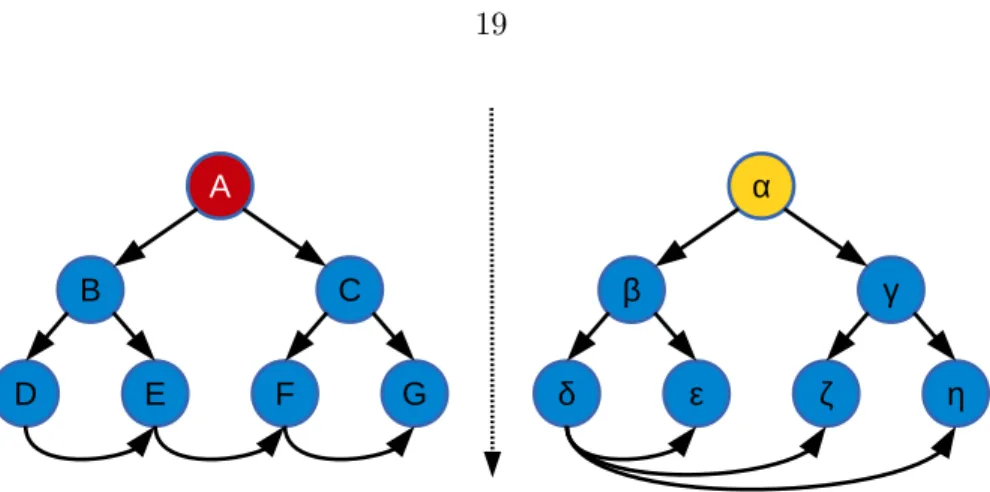
Both neighbor set similarities and neighbor vector similarities require node identifiers or node labels to aid the comparison. If two nodes do not share common neighbor identifiers or neighbor labels, the distance will be always 0. For example, in Figure 3.2, the similarity
Figure 3.2: How similar between A and α?
between node A and nodeα is 0 when using neighbor set similarities and neighbor vector similarities. To address such problem, there is another kind of measurements which extract the features from local neighborhood structures and compare the feature vectors as the node similarity.
Akoglu et al. [1] propose an “OddBall” algorithm to detect abnormal nodes in the graph. In “OddBall” algorithm, the feature vector is constructed by using egonet features which include: degree of the node, number of edges in egonet, total weights of egonet and principal eigenvalue of the weighted adjacency matrix of egonet.
Berlingerio et al. [8] propose a “NetSimile” method which also extracts the feature vectors from nodes’ egonets. But compared to “OddBall”, “NetSimile” extracts 7 features: degree, clustering coefficient, average degree of neighbors, average clustering coefficient of neighbors, number of edges in ego-network, number of outgoing edges of ego-network and number of neighbors of ego-network.
For the geometric graphs which include spatial information, Armiti and Gertz [4] extract lengths and angles information from edges of egonet and construct the vertex features. Then by using string edit distance, the vertex distance is calculated based on their vertex features.
All of above methods extract the features from the egonet which only includes the instant neighbors of a node. Sometimes, more features from a broader neighborhood struc-ture are needed.
Henderson et al. [43] propose a recursive structural features called “ReFex” which recursively combines local features with neighborhood features to construct regional fea-tures that capture “behavioral” information. They separate structural attributes into three types: local, egonet and recursive features. Local and egonet features together are called neighborhood features, and all three together are called regional features. In the neigh-borhood features, local feature is the node degree and egonet features include number of within-egonet edges, as well as number of edges entering and leaving the egonet. While in the recursive features, “ReFeX” collects two types of recursive features: means and sums. They also have a pruning strategy to reduce number of recursive features in “ReFeX”.
All above feature-based similarities can compare two nodes in two different graphs without any label or identity information. Such kind of measures solve the issue raised in Figure 3.2 and feature-based measures could solve problems like graph de-anonymization and transfer learning.
3.5.4 Path-based Similarity
Another type of similarities focuses on local neighborhood structures is called path-based similarity. Path-based similarity needs specific path schemes and node types to measure a pair of nodes. PathSim [113] is a path-based similarity measurement between two nodes in a single connected graph. PathSim utilizes a symmetric meta path to define the node similarity between a pair of nodes in the same type. HeteSim [109] is also a path-based sim-ilarity which measures two nodes in heterogeneous graphs as PathSim. However HeteSim adopts relevance path which can be asymmetric to measure the node similarity.
3.5.5 Role-based Similarity
There is a graph mining task called node role mining. Such task is quite related to the neighborhood-based node similarity measurements. Because if one node is assigned a role, other similar nodes (by using neighborhood-based node similarity measurements) to this node can be assigned to the same role. In the opposite way, the node similarity can be
defined by using the node roles.
Henderson et al. [42] propose “RolX”, an unsupervised approach for automatically extracting structural roles from a graph. In their approach each node is assigned a mixed-membership of roles which means, if there are totallyrdifferent roles, the role of each node can be represented as ar-dimensional vector and each element in the vector is the weight of each role. The roles are clusters or groups of nodes and number of roles r should be pre-specified in the approach. “RolX” consists of three components: feature extraction, feature grouping and model selection. Each node has a feature vector which represents the neighborhood structural information. “RolX” adopts the vectorization method in [43] for feature extraction. Let a node-feature matrix be Vn×f wheren is number of nodes and f
is number of features per node. The feature grouping is to findGand F satisfying:
argmin
G,F k
Vn×f −Gn×rFr×f k s.t. G≥0, F ≥0 (3.7)
wherer is number of roles.
A structural similarity can be defined based on node roles. Since each node can be represented as a vector of mixed-membership of roles. By comparing the distribution over the set of extracted roles, the similarity between two nodes can be measured.
There are some other node role discovery methods. Gilpin et al. [32] consider the supervision in role discovery, where the node role discovery can refer the expert knowledge. Scripps et al. [106] adopt degrees and community scores to construct 4 types of community-based roles: “Ambassadors”, “Big Fish”, “Bridges” and “Loners”. While Chou et al. [19] discover 3 kinds of community-based roles: “Bridges”, “Gateways” and “Hubs” by using topological information.
3.5.6 Graphlets-based Similarity
In biological networks, such as protein-protein interaction networks (PPI), gene regulatory networks, and metabolic networks, finding a mapping from the nodes of one network to the
Table 3.1: Node Similarity Applicability Comparison
Similarity Inter-G Extra-Info Tri-Ineq
SimRank [45] No No No P-Rank [143] No No No PSimRank [28] No No No SimRank++ [3] No No No MatchSim [75] No No No SimRank* [134] No No No RoleSim [46] No No Yes
HITS-based Similarity [12, 137, 89] Yes No No
Random Walk with Restart [92, 118] No No No
Personalized PageRank [40] No No NO
Similarity Flooding [84] Yes Edge Label NO
Sampling-based Similarity [140, 93] No No No Neighbor Set Similarity [79, 110, 127, 127] Yes Node Identifier Yes Neighbor Vector Similarity [80, 49, 50] Yes Node Label No
OddBall [1] Yes No Yes
NetSimile [8] Yes No Yes
Geometric Feature-based Similarity [4] Yes Edge Length Yes
ReFex [43] Yes No No
Path-based Similarity [113, 109] No Node Type No Role-based Similarity [42, 32, 106, 19] Yes Node Role Yes Graphlets-based Similarity [23] Yes Graphlets Yes
nodes of another network is a basic problem in order to align the pairwise networks [21]. Such technique is useful in identifying previously undiscovered homologies between pro-teins of different species and revealing functionally similar subnetworks. Graphlets-based similarity is a typical way to find the node similarity between pairwise nodes. Graphlets are small connected non-isomorphic induced subgraphs of a large network [97] and gener-alize the notion of the degree of a node. For example: [82, 23] extract feature vectors by using graphlets. Davis et al. [23] adopts 30 graphlets and their 73 automorphism orbits to construct the feature vectors of nodes in protein-protein interaction networks. However, they are also limited to the small neighborhood around each node and as the size of the neighborhood increases the accuracy of this method decreases.
3.6 Discussion
Clearly, different applications need different node similarity measurements and different node similarity measurements have different applicabilities. In the discussion, the node similarities discussed above are majorly compared from 3 aspects:
• Whether node similarity can compare two nodes in two different graphs ?
• Whether node similarity can compare two nodes without any extra information ?
• Whether node similarity can rank more than two nodes ?
Be more specific, the first question asks “if two nodes are not reachable, whether the node similarity will always return 0”. The second question asks “What kind of information is needed to let the node similarity work”. The third question asks “Whether two similar-ities of two different pairs of nodes are comparable (or even satisfy triangular-inequality)” Table 3.1 summarizes the existing node similarities based on the questions raised above. If the similarity is able to compare two nodes in two different graphs, in the column “Inter-G”, it is “Yes”. Otherwise, it is “No”. If the similarity does not need any extra information except the topological structure, in the column “Extra-Info”, it is “No”. Otherwise, the extra information needed is listed. If the similarity satisfies the triangular-inequality, in the column “Tri-Ineq”, it is “Yes”. Otherwise, it is “No”.
A Novel Node Metric: NED
4.1 Introduction
Node similarity is a fundamental problem in graph data analysis. Many applications use node similarity as an essential building block to develop more complex graph data mining algorithms. These applications include node classification, similarity retrieval, and graph matching.
In particular, node similarity measures between nodes in different graphs (inter-graph nodes) can have many important applications including transfer learning across networks and graph de-anonymization [43]. An example comes from biological networks. It has been recognized that the topological (neighborhood) structure of a node in a biological network (e.g., a PPI network) is related to the functional and biological properties of the node [23]. Furthermore, with the increasing production of new biological data and networks, there is an increasing need to find nodes in these new networks that have similar topological structures (via similarity search) with nodes in already analyzed and explored networks [21]. Notice that additional information on the nodes can be used to enhance the distance function which uses the network structure around the node. Another application comes from communication networks. Consider a set of IP communication graphs from different days or different networks have been collected and only one of these networks has been analyzed [43]. For example, nodes in one network may have been classified into classes or roles based on their neighborhood. The question is how to use this information to classify nodes from the other networks without the need to build new classifiers (e.g.,
across-network classification) [43]. Finally, another important application of inter-graph node similarity is to use it for de-anonymization. As an example, given an anonymous social network and a non-anonymized social graph in the same domain, comparing pairwise nodes is able to de-anonymize or re-identify the nodes in the anonymous social network by using the structural information from the non-anonymized communication graph [43].
In recent years, many similarity measures for nodes in graphs have been proposed but most of them work only for nodes in the same graphs (intra-graph.) Examples include SimRank [45], SimRank variants [134, 3, 46], random walks with restart [118], and set matching methods [79, 110, 127, 49, 50]. Unfortunately these methods cannot be used for inter-graph nodes. Existing methods that can be used for inter-graph similarity [1, 8, 43, 12], they all have certain problems. OddBall [1] and NetSimile [8] only consider the features in the ego-net (instant neighbors) which limits the neighborhood information. On the other hand, more advanced methods that consider larger neighborhood structures around nodes, like ReFeX [43] and HITS-based similarity [12] are not metric distances and the distance values between different pairs are not comparable. Furthermore, the distance values are not easy to interpret.
This chapter proposes a novel distance function for measuring inter-graph node similar-ity with edit distance, called NED. In NED measure, two inter-graph nodes are compared according to their neighborhood topological structures which are represented as unordered
k-adjacent trees. In particular, the NED between a pair of inter-graph nodes is equal to a modified tree edit distance called TED* that is also proposed in this chapter. Introduc-ing the TED* is because the computation of the original tree edit distance on unordered
k-adjacent trees belongs to NP-Complete. TED* is not only polynomially computable, but it also preserves all metric properties as the original tree edit distance does. TED* is empirically demonstrated to be efficient and effective when comparing trees. Compared to existing inter-graph node similarity measures, NED is a metric and therefore can admit efficient indexing and provides results that are interpretable, since it is based on edit dis-tance. Moreover, since the depth of the neighborhood structure around each node can be
parameterized, NED provides better quality results in the experiments, including better precision on graph de-anonymization. A detailed experimental evaluation is provided to show the efficiency and effectiveness of NED using a number of real-world graphs.
Overall, this chapter makes the following contributions:
[1] Propose a novel distance function, NED, to measure the similarity between inter-graph nodes.
[2] Propose a modified tree edit distance, TED*, on unordered trees that is both metric and polynomially computable.
[3] By using TED*, NED is an interpretable and precise node similarity that can capture the neighborhood topological differences.
[4] Show that NED can admit efficient indexing for similarity retrieval.
[5] Experimentally evaluate NED using real datasets and show that it performs better than existing approaches on a de-anonymization application.
The rest of this chapter is organized as follows. Section 4.2 introduces related work of node similarity measurements. Section 4.3 proposes the unordered k-adjacent tree, inter-graph node similarity with edit distance which is called as NED in this chapter and the NED in directed graphs. Section 4.4 introduces TED*, a modified tree edit distance, and its edit operations. Section 4.5 elaborates the detailed algorithms for computing TED*. Section 4.6 presents the correctness proof of the algorithm and Section 4.7 proves the metric properties of TED*. Section 4.8 illustrates the isomorphism computability issue when comparing node similarities. Section 4.9 provides the analysis of the complexities and Section 4.10 introduces the analysis of the only parameterkin NED and the monotonicity property in NED. Section 4.11 theoretically compares the TED* proposed in this chapter with TED and GED from two aspects: edit operations and edit distances. Section 4.12 proposes a weighted version of NED. Section 4.13 empirically verifies the effectiveness and efficiency of TED* and NED. Section 4.14 concludes the whole chapter and Section 4.15 proposes the future work.
4.2 Related Work
One major type of node similarity measure is called link-based similarity or transitivity-based similarity and is designed to compare intra-graph nodes. SimRank [45] and a number of SimRank variants like SimRank* [134], SimRank++ [3], RoleSim [46], just to name a few, are typical based similarities which have been studied extensively. Other link-based similarities include random walks with restart [118] and path-link-based similarity [113]. A comparative study for link-based node similarities can be found in [77]. Unfortunately, those link-based node similarities are not suitable for comparing inter-graph nodes since these nodes are not connected and the distances will be always 0.
To compare inter-graph nodes, neighborhood-based similarities have been used. Some primitive methods directly compare the ego-nets (direct neighbors) of two nodes using Jaccard coefficient, Sørensen–Dice coefficient, or Ochiai coefficient [79, 110, 127]. Ness [49] and NeMa [50] expand on this idea and they use the structure of thek-hop neighborhood of each node. However, for all these methods, if two nodes do not share common neighbors (or neighbors with the same labels), the distance will always be 0, even if the neighborhoods are isomorphic to each other.
An approach that can work for inter-graph nodes is to extract features from each node using the neighborhood structure and compare these features. OddBall [1] and NetSimile [8] construct the feature vectors by using the ego-nets (direct neighbors) information such as the degree of the node, the number of edges in the ego-net and so on. ReFeX [43] is a framework to construct the structural features recursively. The main problem with this approach is that the choice of features is ad-hoc and the distance function is not easy to interpret. Furthermore, in many cases, the distance function may be zero even for nodes with different neighborhoods. Actually, for the more advanced method, ReFeX, the distance method is not even a metric distance.
Another method that has been used for comparing biological networks, such as protein-protein interaction networks (PPI) and metabolic networks, is to extract a feature vector
using graphlets [82, 23]. Graphlets are small connected non-isomorphic induced subgraphs of a large network [97] and generalize the notion of the degree of a node. However, they are also limited to the small neighborhood around each node and as the size of the neighborhood increases the accuracy of this method decreases.
Another node similarity for inter-graph nodes based only on the network structure is proposed by Blondel et al. [12] which is called HITS-based similarity. In HITS-based similarity, all pairs of nodes between two graphs are virtually connected. The similarity between a pair of inter-graph nodes is calculated using the following similarity matrix:
Sk+1 =BSkAT +BTSkA
whereAandB are the adjacency matrices of the two graphs andSkis the similarity matrix
in thek iteration.
Both HITS-based and Feature-based similarities are capable to compare inter-graph nodes without any additional assumption. However, HITS-based similarity is neither metric nor efficient. On the other hand, Feature-based similarities use ad-hoc statistical informa-tion which cannot distinguish minor topological differences. This means that Feature-based similarities may treat two nodes as equivalent even though they have different neighborhood structures.
4.3 NED: Inter-Graph Node Similarity with Edit Distance
4.3.1 K-Adjacent Tree
First of all, this section introduces the unlabeled unordered k-adjacent tree that is used to represent the neighborhood topological structure of each node. The k-adjacent tree was firstly proposed by Wang et al. [122] and for the completeness, the definition is included here:
Figure 4.1: K-Adjacent Tree
search tree starting from vertex v. The k-adjacent tree T(v, k) of a vertex v in graph
G(V, E) is the top k-level subtree of T(v).
The difference between the k-adjacent tree in [122] and the unlabeled unordered k -adjacent tree used in this chapter is that the children of each node are not sorted based on their labels. Thus, thek-adjacent tree used in this chapter is an unordered unlabeled tree structure.
An example of a k-adjacent tree is illustrated in Figure 4.1. For a given node in a graph, its k-adjacent tree can be retrieved deterministically by using breadth first search. In this chapter, the tree structure is used to represent the topological neighborhood of a node that reflects its “signature” or “behavior” inside the graph.
In the following chapter the undirected graphs are considered for simplicity. However, thek-adjacent tree can also be extracted from directed graphs. Furthermore, the distance metric can also be applied to directed graphs as discussed in Section 4.3.3. Later, Section 4.8 explains why a tree rather than the actual graph structure around a node is chosen as the node signature.
4.3.2 NED
Here, NED, the inter-graph node similarity with edit distance, is introduced. Let u and
v be two nodes from two graphs Gu and Gv respectively. For a given parameter k, two k-adjacent trees T(u, k) and T(v, k) of nodesu and v can be generated separately. Then, by applying the modified tree edit distance TED* on the pair of twok-adjacent trees, the similarity between the pair of nodes is defined as the similarity between the pair of the two
k-adjacent trees.
Denote δk as the distance function NED between two nodes with parameter k and denoteδT as the modified tree edit distance TED* between two trees. Then for a parameter k,
δk(u, v) =δT(T(u, k), T(v, k)) (4.1)
Notice that, the modified tree edit distance TED* is a generic distance for tree struc-tures. In the following sections, the definition and algorithms for computing the proposed modified tree edit distance are described in details.
4.3.3 NED in Directed Graphs
This chapter discusses the inter-graph node similarity for undirected graphs. The k -adjacent tree is also defined in undirected graphs. However it is possible to extend the
k-adjacent tree and inter-graph node similarity from undirected graphs to directed graphs. For directed graphs, there are two types ofk-adjacent trees: incomingk-adjacent tree and outgoingk-adjacent tree. The definition of incomingk-adjacent tree is as follows:
Definition 3. The incoming adjacent treeTI(v)of a vertexvin graphG(V, E)is a
breadth-first search tree of vertexv with incoming edges only. The incomingk-adjacent treeTI(v, k) of a vertex v in graph G(V, E) is the top k-level subtree of TI(v).
Similarly, the outgoing adjacent tree TO(v) includes outgoing edges only. For a given
node in a directed graph, both incomingk-adjacent tree and outgoingk-adjacent tree can be deterministically extracted by using breadth-first search on incoming edges or outgoing edges only.
Based on Definition 3, for a node v, there are two k-adjacent trees: TI(v) and TO(v).
Letube a node in the directed graph Gu andv be a node in the directed graphGv. Then
the distance function NEDδDk in directed graphs can be defined as:
Notice that, since TED* is proved to be a metric, not only the NED defined in undi-rected graphs is a node metric, but the NED defined in diundi-rected graphs is also a node metric. The identity, non-negativity, symmetry and triangular inequality all preserve according to the above definition.
4.4 TED*: Modified Tree Edit Distance
The tree edit distance [115] is a well-defined and popular metric for tree structures. For a given pair of trees, the tree edit distance is the minimal number of edit operations which convert one tree into the other. The edit operations in the original tree edit distance include: 1) Insert a node; 2) Delete a node; and 3) Rename a node. For unlabeled trees, there is no rename operation.
Although the ordered tree edit distance can be calculated inO(n3) [95], the computation
of unordered tree edit distance has been proved to belong toNP-Complete [142], and even MaxSNP-Hard [141]. Therefore, a novel modified tree edit distance called TED* is proposed which still satisfies the metric properties but it is also polynomially computable.
The edit operations in TED* are different from the edit operations in the original tree edit distance. In particular, TED* does not allow any operation that can change the depth of any existing node in the trees. The reason is that, the depth of a neighbor node, which should be an important property of this node in the neighborhood topology, represents the closeness between the neighbor node and the root node. Therefore, two nodes with different depths should not be matched. The definition of TED* is below:
where each edit operation ei belongs to the set of edit operations defined in Section
4.4.1. |E|is the number of edit operations in E and δT is the TED* distance proposed in
Figure 4.2: TED* vs Tree Edit Distance
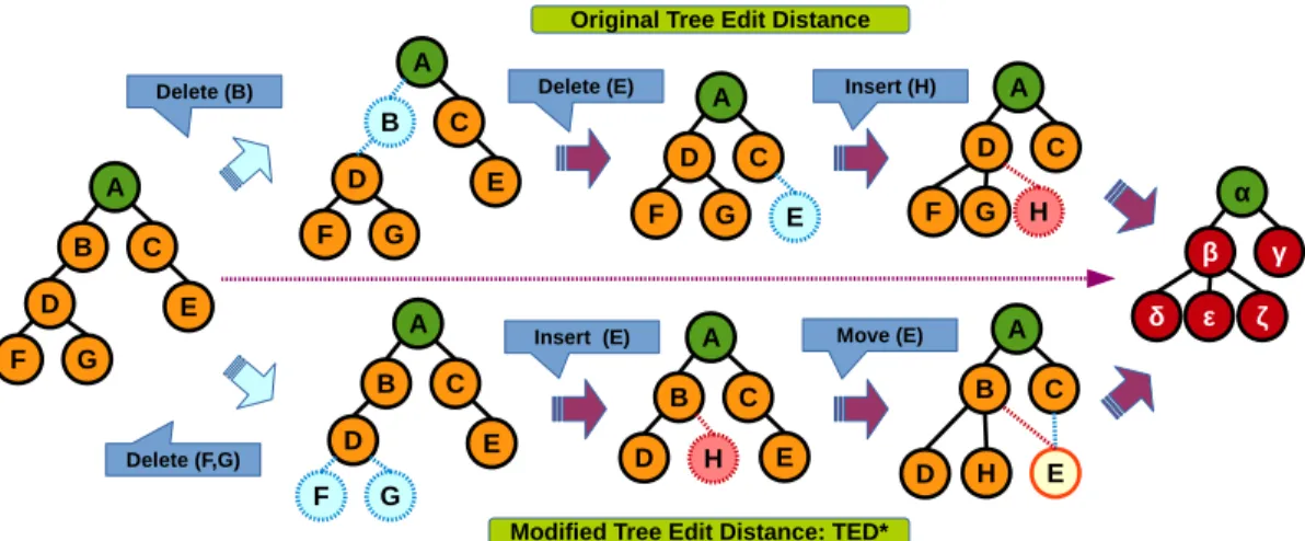
4.4.1 Edit Operations in TED*
In the original tree edit distance, when inserting a node between an existing nodenand its parent, it increases the depth of nodenand also increases the depths of all the descendants of noden. Similarly, when deleting a node which has descendants, it decreases the depths of all the descendants. Since in TED* no operation can change the depth of any existing node, those operations should not be allowed. Therefore, another set of edit operations is needed as follows:
I: Insert a leaf node II: Delete a leaf node
III: Move a node at the same level
To clarify, “Move a node at the same level” means changing an existing node’s parent to another. The new parent node should be in the same level as the previous parent node. The above 3 modified edit operations do not change the depth of any existing node. Also after any edit operation, the tree structure is preserved.
Figure 4.2 shows an example of the difference between the traditional tree edit distance and the modified tree edit distance in this chapter. When converting the tree Tα to the
node E and insert node H. TED* requires 4 edit operations: delete node F, delete node
G, insert nodeH and move node E.
Notice that, for the same pair of trees, TED* may be smaller or larger than the original tree edit distance. Section 4.11 analyzes the differences among TED*, the original tree edit distance and the graph edit distance in more details, where the TED* can be used to provide an upper-bound for the graph edit distance on trees.
In the following of this chapter number of edit operations is considered in TED* which means each edit operation in TED* has a unit cost. However, it is easy to extend TED* to a weighted version. Section 4.12 introduces the weighted TED*. The weighted TED* can be proven to be a metric too and moreover, the weighted TED* can provide an upper-bound for the original tree edit distance.
Definition 4. Given two trees T1 and T2, a series of edit operations E = {e1, ...en} is
valid denoted as Ev, if T1 can be converted into an isomorphic tree of T2 by applying the edit operations in E. Then δT(T1, T2) = min|E|, ∀Ev.
4.5 TED* Computation
This section introduces the algorithm to compute TED* between a pair ofk-adjacent trees. It is easy to extend TED* to compare two generic unordered trees. Before illustrating the algorithm, some definitions are introduced.
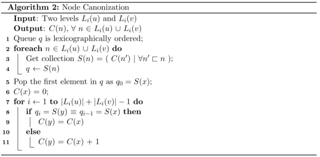
Definition 5. Let Li(u) be the i-th level of the k-adjacent tree T(u, k), where Li(u) =
{n|n∈T(u, k), d(n, u) =i} and d(n, u) is the depth of node nin T(u, k).
In Definition 5, thei-th levelLi(u) includes the nodes with depths ofiin thek-adjacent
tree T(u, k). Similarly in k-adjacent tree T(v, k), there exists the i-th level Li(v). The
algorithm compares twok-adjacent treesT(u, k) andT(v, k) bottom-up and level by level. First, the algorithm compares and matches the two bottom levels Lk(u) andLk(v). Then
the next levels Lk−1(u) andLk−1(v) are compared and matched. The algorithm continues