EPRU Working Paper Series
2007-02
Economic Policy Research Unit Department of Economics University of Copenhagen Studiestræde 6 DK-1455 Copenhagen K DENMARK Tel: (+45) 3532 4411 Fax: (+45) 3532 4444 Web: http://www.econ.ku.dk/epru/
How do Capital Controls Affect the Transmission
of Foreign Shocks?
Dudley Cooke
How do Capital Controls Affect the
Trans-mission of Foreign Shocks?
∗Dudley Cooke†
University of Essex April 2007
Abstract: This paper studies the short-run transmission of foreign shocks in a small open economy with capital controls and a fixed exchange rate. Capital controls alter the trans-mission of shocks because endogenous changes in the domestic nominal interest rate affect savings and investment decisions. The economy’s reaction to export shocks hinges on how the government chooses to restrict capital flows; that is, whether inflows or outflows are re-stricted. For foreign interest rate shocks, private capital flows are important, but so are the government’s holdings of foreign exchange reserves. Finally, a simple graphical apparatus is developed to provide a contrast to the case when capital flows are unrestricted.
JEL Classification: E58, F32, F41.
Keywords: Capital Controls, Foreign Shocks.
∗This paper was partly written whist I was based at the University of Copenhagen, funded by the
European Commission RTN ‘Macroeconomic Policy Design for Monetary Unions’. I would very much like to thank the Department of Economics for providing a stimulating research environment. Thanks also to Neil Rankin, Philip Lane, and seminar participants at Birmingham, Oxford, Trinity College Dublin, Warwick, and the 2005 LACEA and 2007 RES conferences.
†Department of Economics, University of Essex, Wivenhoe Park, Colchester CO4 3SQ, UK. Email:
1. Introduction
The exchange rate regime and degree of capital mobility take centre stage when thinking about an economy’s exposure to foreign shocks. Recently, a number of attempts have been made to either develop, or improve on, the IMF’s Annual Report on Exchange Arrangements and Exchange Restrictions, which provides dejure measures for both of these. Along one dimension, Reinhart and Rogoff (2004) and Levy-Yeyati and Sturzenegger (2005) present defacto classifications of exchange rate regimes.1 Along the other, Lane and Milesi-Ferretti’s (2001, 2006) work, documenting countries’ net external wealth positions, leads to a defacto index of capital account openness. These studies show that, although financial market integration has risen, capital controls, in one form or another, are still used in a majority of countries. Capital controls are also often used to support a managed exchange rate.2 Given this, it is an important task to understand exactly how capital controls affect an economy’s reaction to foreign shocks.3
This paper uses a sticky-price model of a small open economy to investigate the short-run transmission of foreign shocks, when the exchange rate is fixed, and the government imposes a capital control. The capital control is introduced through a separate exchange rate ap-plied to financial transactions; that is, a dual exchange rate system. It is well-known that dual exchange rates and capital controls are formally equivalent, but an important contribu-tion of this paper is to show that by integrating capital controls into a model with nominal rigidities, monopolistic competition, and physical capital, there is also an equivalence be-tween the textbook Mundell-Fleming and DGE approaches.4 Without capital controls, a balance-of-payments condition, similar to that presented in C´espedes et al. (2004), deter-mines investment behavior, consumption is pinned down by an investment-savings condition, and when prices are sticky, output is determined by current levels of demand. When the exchange rate is fixed, money demand determines the level of money supply residually. With capital controls, investment demand is decreasing in the domestic interest rate. Given the
1Reinhart and Rogoff (2004) argue that 50% of official pegs float through the use of dual exchange rates,
whereas Levy-Yeyati and Sturzennegger (2005) cite hidden pegs and fear of floating as prevalent.
2Alesinaet al. (1993) discuss the political economy aspects of this situation.
3Miniane (2004) develops a detailed dejure measure of capital account restrictions and Miniane and
Rogers (2007) use this to assess whether capital controls insulate domestic countries’ interest rates from U.S. monetary shocks.
4This intertemporal equivalence is first shown in Adams and Greenwood (1985). I use the terms ‘dual
investment-savings relationship, and sticky prices, investment demand is increasing in out-put; or rather, the balance-of-payments relationship is ‘upward-sloped’. In addition to the usual national intertemporal budget constraint, a period national budget constraint, link-ing government reserves to the flow of private capital, is also required to hold when there are capital controls. Because the money supply is tied to the flow of government reserves, money demand becomes central in determining the equilibrium, even if the exchange rate is fixed. Thus, the DGE model developed here, generates familiar looking IS, BP, and LM conditions, when there are capital controls. The important difference is that household and firm conditions are derived from optimizing behavior, and the private sector distortions and public sector revenues that capital controls introduce are accounted for through budget constraints.
Two foreign shocks are studied; export shocks and foreign interest rate shocks. The key mechanism that alters the reaction of the economy to these shocks is the (endogenous) change in the domestic nominal interest rate. An adverse shock to exports, taken to represent lower global demand for the domestic commodity or, more loosely, a tariff imposed on sales -reduces GDP by more than it does with unrestricted capital flows, whenever the government imposes a capital outflow. In this case, investment reacts by more than output because, to force the outflow of private capital, the government needs to allow the domestic interest rate to rise. This reinforces the negative effects of the shock and, in this sense, capital controls add to the variability of output. Regardless of the restriction on the flow of capital, the domestic interest rate and investment fall when the foreign interest rate rises. However, the reaction of consumption depends explicitly on the target the government sets for the capital account, and also its holdings of foreign exchange reserves. Only when the country is neither a net creditor nor debtor internationally is the result unambiguous: consumption is insulated from the shock. When this special case does not hold, consumption may rise or fall with the shock, depending on whether the economy is a net creditor or debtor, respectively. Thus, the often assumed insulation properties of capital controls with regard to GDP and foreign interest rate shocks fail to hold, and the governments holdings of foreign exchange reserves are important for determining the co-movement of macro aggregates.
There is a related literature that studies capital controls in economies with money. The Mundell-Fleming framework emphasizes insulation from foreign interest rate shocks, and the possibility of independent monetary policy. However, using a portfolio-balance ap-proach, Marion (1981), for example, shows that insulation occurs only as a special case,
and Aizenman (1985) shows that limited capital mobility does not necessarily increase the scope for monetary policy, when the exchange rate is fixed. Both the Mundell-Fleming and portfolio-balance model offer useful but limited insights. This is particularly true of the former because it does not account for the flow of net foreign assets. Studies based on this framework cannot disentangle the inflow and outflow of reserves and neither can they explain the implications of temporary capital account restrictions. More closely related to the analysis here, Guidotti and V´egh (1992) analyze capital controls in an explicitly in-tertemporal framework. However, in the representative agent economy they develop output is exogenous. More recently, Calvo et al. (1995) and Reinhart and Smith (2002) study the intertemporal implications of capital controls in economies with traded and non-traded goods.5 Finally, C´espedes et al. (2004) and Lahiri et al. (2006) study the optimality of different exchange rate regimes when capital market imperfections arise in the private sec-tor. The former, incorporates liability dollarization, whereas Lahiri et al. (2006) introduce exogenously segmented asset markets.
The remainder of the paper is organized as follows. Section two describes the model economy. Section three develops a simple representation of the equilibrium conditions of the model and section four studies the reaction of the economy to export and foreign interest rate shocks. Section five concludes.
2. The Model Economy
There is a small domestic economy and a large foreign economy, which exist for two periods.6 Other than their size the domestic and foreign economies are identical.
A. Firms
There are two types of domestic firms; those producing a homogenous final good and those producing a differentiated intermediate good.7 Final good firms have access to the following
5Mendoza (1991) provides an analysis of capital controls in a business cycle model of a small open
economy with technology shocks. The obvious drawback of omitting money is that once the capital account is regulated, so is the current account.
6It would be possible to extend the analysis to an infinite horizon if I were interested in examining the
implications for the length of the capital account restrictions. See Frenkel and Razin (1986) for an analysis of these considerations.
7The analysis of this section draws on the open economy macroeconomics literature that stresses the use
Cobb-Douglas technology,
zt=yh,tn yf,t1−n/nn(1−n)
1−n (1)
wherezt is the final good, andyh,t and yf,t are aggregate bundles of the intermediate goods,
produced in the domestic and foreign economies respectively. These firms maximize profits,
Ptzt−Ph,tyh,t−Pf,tyf,t, choosingyh,t andyf,t, subject to (1), implying the demand functions
for domestic and foreign intermediate goods are,
yh,t =zt(Pt/Ph,t)n (2)
yf,t =zt(Pt/Pf,t) (1−n) (3)
wherePt ≡Ph,tn Pf,t1−n is the consumer price index (CPI) and Ph,t is the price of the domestic
intermediate good. Foreign firms face the same problem, but because of the asymmetry introduced by the small open economy assumptionn∗ →0. In this case, the foreign version
of (1) impliesz∗
t ∼=yf,t∗ , and the corresponding foreign CPI isPt∗ ∼=Pf,t∗ , which is exogenous.
This does not mean exports are zero, because z∗
t itself is large. Using a law of one price
assumption,Ph,t =etPh,t∗ , where et is the goods market exchange rate, export demand is,
yh,t∗ =gt∗(et/Ph,t) (4)
whereg∗
t ≡zt∗n∗ is restricted to be non-zero and finite, and is exogenous from the viewpoint
of the domestic economy. Export demand depends explicitly on the relative price.
The aggregate bundle of intermediate goods is produced using a constant elasticity of sub-stitution production function. For the domestic firm,
yh,t = ·Z 1 0 yh,t(j)(θ−1)/θdj ¸θ/(θ−1) (5) whereyh,t(j) is thejthintermediate input and the parameterθ > 1 measures the substitution
elasticity between types. Profits, Ph,tyh,t −
R1
0 Ph,t(j)yh,t(j)dj, are maximized, choosing
yh,t(j), subject to (5). The solution to this problem implies a downward sloping input
demand function of the form,
yh,t(j) = (Ph,t(j)/Ph,t)−θyh,t (6)
wherePh,t =
³R1
0 Ph,t(j)1−θdj
´1/(1−θ)
is the corresponding price index, derived from the zero profit condition.
The differentiated intermediate goods are produced using competitively supplied domestic labor and capital with a Cobb-Douglas technology.
yh,t(j) +yh,t∗ (j) =ktγlt(j)α (7)
whereγ +α = 1, kt is capital, lt is the labor input, and yt(j) =yh,t(j) +yh,t∗ (j) is domestic
GDP. Intermediate good firms maximize profits,R01Ph,t(j)yt(j)dj−wtlt(j)−Qtkt, choosing kt, lt(j), andPh,t(j), wherewtare nominal wages, andQtis the nominal rental rate of capital,
such that (6) and (7) hold.
Cost minimization implies factor demands can be written as,
kt/lt(j) = [(1−α)/α]wt/Qt (8)
Given factor demand, firm j sets the price of it’s good as a mark-up over marginal cost,
mct.8 In equilibrium, intermediate good firms set the same price,
Ph,t = [θ/(θ−1)]Et−1{mct} for t = 0,1 (9)
whereθ/(θ−1)>1 is the monopoly markup.9 B. Households
Domestic households choose foreign nominal bond and domestic nominal money holdings, consumption, labor supply, and investment. Suppressing thej index, households maximize,
U =u(C0, m0, l0) +βu(C1, m1, l1)
subject to the period budget constraint and capital accumulation equation,
st ¡ ∆Bt−Bt−1i∗t−1 ¢ =ϑt+wtlt+Qtkt−Pt(Ct+xt)−Mt+Mt−1− Tt (10) xt=kt+1 (11)
for t= 0,1. Above, β ∈(0,1) is the discount factor, Ct is total consumption, mt≡ Mt/Pt
are real money balances, xt is investment, so that Ptxt represents nominal expenditure on
8Constant returns to scale in production and perfectly competitive factor markets imply k
t/lt(j) =kt/lt
∀j, with nominal marginal costmct=wtαQγt/ααγγ.
9I write this expression with an expectations operator because although thet= 1 version holds exactly the
t= 0 version may not hold ex-post, given an unanticipated shock. Note also thatmct=wt/fl=wtlt/αktγlαt
capital, and ϑt are monopoly profits from the production of the differentiated intermediate
good. The foreign net nominal interest rate is i∗
t, st is the financial exchange rate, Bt
are foreign currency bonds, so that ∆Bt represents the change in foreign assets holdings
of individual j. Finally, Tt is a nominal lump-sum government tax. In (11), it has been
assumed, for simplicity, that capital depreciates completely in production.
I specialize period utility to u = lnCt +aln (Mt/Pt)−κlt, where a > 0 is a measure of
monetary frictions and κ > 0 is the weight attached to the dis-utility of labor. The first-order conditions imply,
P1C1 =βP0C0(1 +i0) (12)
wt=κPtCt fort = 0,1 (13)
P1C1 =βC0Q1 (14)
M0 =aP0C0(1 +i0)/i0 (15)
M1 =aP1C1 (16)
Equation (12) is the consumption Euler equation, (13) represents labor supply, and (14) the optimal choice of capital.10 Equations (15) and (16) express the demand for money, where money held in the terminal period is independent of the interest rate.
Of the two exchange rates, the financial exchange rate,st, is important for flows of net foreign
assets, and it alone appears in the household budget constraint. Equations (12), (14) and (15) are affected by the financial exchange rate through the domestic nominal interest rate because, in the current period, one unit of domestic currency purchases 1/s0 units of foreign currency, not 1/e0 units. I assume this purchase can only be repatriated the following period at the rates1. During the period, the 1/s0 units earn i∗1/s0 units of interest income, so the amount of foreign currency repatriated into domestic currency is i∗
1s1/s0. The combination of these two returns leads to the following real UIP condition.
q0(1 +r0) =q1(1 +r0∗)/f0 (17)
where qt ≡ et/Pt is the the real exchange rate and f0 ≡ (s0/e0)/(s1/e1) measures the wedge that distorts intertemporal consumption trade. Using the Fisher equation, (1 +i0) =
10Equivalent to the firms decision I can write,w
(1 +i∗
0)τ0, where τ0 ≡ s0/s1. Whenever the exchange rates are unified f0 = 1, so there is no distortion, despite τ0 6= 1. Whenever the commercial exchange rate is pegged τ0(=f0) can be thought of as the distortion.
C. Government
The government consists of a central bank, an import-export authority (IEA), and an ex-change rate authority (ERA). The central bank-cum-fiscal authority levies lump-sum taxes and transfers, prints money and earns revenue from interest income on reserves. Printing money, issuing credit, and reserve holdings are connected by a balance sheet condition,
Mt−Mt−1 =et·∆Rt+dt−dt−1 (18)
whereRtare foreign exchange reserves anddtis domestic credit. The exchange rate attached
to reserves is that associated with commercial transactions because the government is free to enter the foreign exchange market without restriction. The central banks period budget constraint is,
Tt=dt−1−dt−etRti∗t−1 for t = 0,1 (19)
Intertemporally, central bank transfers,Tt, are constrained by the initial levels of the money
supply and reserves, seigniorage revenues and (interest) income lost due to issuing money. The IEA restricts intratemporal trade in domestic and foreign goods, thereby eliminating the possibility of arbitrage between the commercial and financial exchange rates.11 The ERA restricts intertemporal trade. If a domestic resident wants to exchange one unit ofperiod t domestic output forforeign currency bonds in order to consume one unit of theperiod t +1 foreign output, one unit of domestic output is taken to the ERA, who, in exchange for it’s
11If a domestic resident wants to export one unit of the period t domestic output in exchange for one
unit ofperiod t foreign output they take the unit of domestic output to the IEA, where its foreign currency value isPh,t/et. The foreign currency is then used to purchase foreign output, through the IEA, and at
the foreign currency price, P∗
f,t per unit. Agents hold foreign currency whilst interacting with the IEA
and are prevented from interacting with foreign residents directly. Domestic residents are also prevented from obtaining foreign currency (at the exchange rate et) in order to buy foreign bonds (at the exchange
ratest) eliminating arbitrage possibilities. The IEA is not assumed to earn revenue for the government
despite its role as the economy’s monopoly supplier of the foreign output. If it did this would be equivalent to imposing a tariff on imports. See Fender and Yip (2000) for an analysis of goods market tariffs in a sticky-price environment.
domestic currency value,Ph,t, issues a credit ofPh,t/st units of foreign currency. Interest is
paid on the credit so that in period t+ 1 the foreign bond pays back (1 +i∗
t)Ph,t/st units of
foreign currency and the domestic resident receives (1 +it)Ph,t units of domestic currency.12
The ERA generates revenue from these actions because in period t, for one unit of the do-mestic output, Ph,t/st units of foreign currency are credited to the domestic resident. This
unit is sold to foreign residents forP∗
h,t. Using the LOP assumption, the profit made on the
transaction is [1−(et/st)]Ph,t∗ . The ERA buys back the foreign bond from the domestic
res-ident in periodt+ 1 paying out domestic currency to the value of (1 +i∗
t) (st+1/st)Ph,t/Pf,t+1 units of foreign output. The ERA then redeems the bond with the foreign issuers and receives (1 +i∗
t)Ph,t/st units of foreign currency. But this amount of currency buys (1 + i∗
t) (1/st)Ph,t/Pf,t∗ +1 units of foreign output on world markets and the profit on the redemp-tion is, (1 +it) [(st+1/et+1)−1]etPh,t∗ .
Therefore, by settingst> et, the ERAs actions make it more expensive for domestic residents
to gain a credit of one unit of foreign output today than to actually buy and consume that unit. But, by setting st+1 < et+1, domestic residents who cash in their bonds receive less, in terms of foreign output, than the amount which the bonds would yield if domestic agents were able to directly interact with foreign agents. Combining the general profit level of the ERA with the resources available to the domestic residents the ERA period constraint is,
Tt= (et−st)
¡
∆Bt−Bt−1i∗t−1
¢
for t= 0,1 (20)
This is the counterpart of the central bank’s period constraint, and wheneverst6=et, private
bond holdings create revenue which is reflected in the difference between domestic and foreign rates of return on financial investments. However, as stressed before, it is the ratio of the percentage change of the two exchange rates that distorts capital markets.
D. Equilibrium
The resource constraint is zt = Ct+
R1
0 xt(j)dj. Using the intratemporal micro-demand conditions, and the definition of domestic GDP, the goods market equilibrium condition is,
ytPh,t =n(Ct+kt+1)Pt+etgt∗ (21)
where kt+1 =xt and x1 = 0 such that future output on the demand-side is independent of the level of investment.
12The ERA finances this action by buying foreign bonds to the valueP
Wages are flexible, and an economy-wide supply curve relating output, consumption, and capital holds each period.
yt=kt{[θκ/(θ−1)α]CtPt/Ph,t}α/(α−1) (22)
Both the goods and labor market equilibrium conditions link output, consumption and in-vestment to relative prices. When the price is set one period in advance, in the current period, and for a given stock of capital, (21) alone determines the level of output and g∗
t
can be thought of as a demand-shifter. To determine investment, factor demands need to be included. In the future period, due to perfect foresight, the goods and labor market equilibrium conditions, and factor demands, determine output.
Finally, solving the government and individual budget constraints forward, gives the national intertemporal budget constraint (NIBC).
0 = 1 X t=0 ¡ Ph,tyh,t∗ −Pf,tyf,t ¢ /£(1 +i∗ 0)... ¡ 1 +i∗ t−1 ¢¤ (23) wherePh,tyh,t∗ −Pf,tyf,tis net exports, (1 +i∗0)...
¡
1 +i∗
t−1
¢
≡1 whent= 0, and (R1+B1) = 0 replaces the no Ponzi-game condition. From (23), the discounted sum of the trade balance (evaluated using the foreign interest rate) is equal to the initial economy-wide net foreign asset position.
3. Capital Controls
The central bank fixes the exchange rate through reserve transactions, and the IEA and ERA segment the goods and bond markets so that the government can restrict the flow of private capital.13 As usual, the NIBC needs to hold, however, with capital controls, so does a period national budget constraint (NBC). The NBC can be expressed in the following way.
∆R =CA0+ ∆B (24)
This constraint has a very standard interpretation: the balance-of-payments, ∆R, equals the sum of the current account, CA0, and the capital account, ∆B. As the initial level
13One might imagine there is a degree of imperfection in separation, which is more realistic. However,
for clarity, it is more natural to consider polar cases without speculating on the scope of government control over goods and financial markets. Dornbusch (1988) explains this segmentation idea in greater detail.
of economy-wide debt is zero, Phyh,∗0 −Pf,0yf,0, which is the trade balance, also measures the current account, which we normally think of as, Phyh,∗0 − Pf,0yf,0 +i∗−1B−1. When
Phyh,∗0 > Pf,0yf,0, there is a current account surplus. The change in private agents holdings of net foreign assets,B0−B−1, is now captured byB0. WhenB0 >0 domestic residents buy foreign bonds and there is a capital outflow. When B0 <0 domestic residents sell foreign bonds and there is a capital inflow. Above, ∆B ≡ −B0, and thus, ∆B > 0 represents a capital inflow, and ∆B < 0 a capital outflow.14 Finally, since reserves are used to fix the exchange rate,CA0 6= ∆B. Above, R0 −R−1 =R0 ≡∆R. If ∆R >0, the government is accumulating reserves, and the balance-of-payments is in surplus. When ∆R < 0, there is a balance-of-payments deficit.15
The reserve position of the government also needs to be consistent with the central banks balance sheet because reserve holdings are simply the sum of domestic credit and the money supply,M0 = ∆R+D0. This implies the following condition holds when the aggregate flow of private capital is restricted to ∆B.
∆B =P C0 · a µ 1 +i∗ 0 (1 +i∗ 0)−τ0 ¶ + (1−n) ¸ + (1−n)P x0−(eg0∗+D0) (25)
This condition implies there is an economy-wide (aggregate) limit to lending; ∆B cannot be ‘too’ negative. In particular, we cannot lend more than the sum of the economy’s holdings of current credit and the current level of exports in nominal terms; ∆B > −(eg∗
0 +D0). Recall, eg∗
0 ≥ 0 is exogenous, as is D0 ≥ 0, but this is a policy variable. Thus, it is possible for ∆B → −∞, but only if either exports are very high, or the level of credit is expanded. It is permissible for ∆B → +∞ for any eg∗
0 ≥ 0, D0 ≥ 0; that is, the government is not restricted in how much the economy borrows today (the extent of capital inflows). Finally, with unrestricted private capital flows, the NIBC alone matters for the net foreign asset position of the economy. When capital controls are imposed, money demand becomes central to determining the behavior of output, through the NBC, which relates to the balance-of-payments.
The determination of consumption and investment is more standard. Using the consump-tion Euler and nominal UIP equaconsump-tions, the NIBC can be expressed in terms of current consumption, the change in the financial exchange rate, and investment, consistent with the
14Likewise, ∆B >0 is a capital account surplus, and ∆B <0 a deficit. 15From this we can also write the NIBC as, −CA
intertemporal approach to modelling the current account. This only leaves investment de-mand. The approach adopted in this paper is related to C´espedeset al. (2004), in that the factor demand and price setting conditions are used to determine future nominal output as a function of investment and the domestic nominal interest rate. Goods market equilibrium then provides a second condition in these variables, once it is itself combined with the NIBC. This second step is important because although, in aggregate, private agents holdings of net foreign assets are determined by government policy, and therefore constrained by (25), at the individual, level savings are determined endogenously.
A. IS, LM, and BP Schedules
Because the equilibrium conditions of the model are non-linear I describe the economy through conditions linearized around the no-shock equilibrium.16 Output is demand con-strained in the current period, so the goods market equilibrium condition and NIBC produce an IS equation in output, investment and the domestic nominal interest rate. Since the do-mestic interest rate is related, via UIP, to the tax on financial asset transactions, the IS condition is written in the following way.
b
y0 =ρg∗bg∗−ρi∗bi∗0+ρxbx0+ρττb0 (26)
where a circumflex denotes the percentage deviation from the no-shock equilibrium. The coefficients, which are functions of underlying structural parameters, and the policy variable, ∆B, lie between zero and one.17 The restriction ρ
x+ρg∗ = 1 holds for the IS parameters
because firms have access to Cobb-Douglas technologies and the export shock is permanent. Output is increasing in investment and exports and decreasing in the foreign interest rate and the tax on foreign financial assets.
In linear form the BP equation has the following representation.
b
x0 =bg∗−λi∗bi∗0+λτbτ0 (27)
16Since the focus of the analysis is on the initial impact of shocks I do not include the analysis of the
long-run here. Moreover, it seems natural to focus on the initial reaction of the economy (when output is demand determined), given that capital controls are an inherently short-run phenomenon.
17Because the model is non-linear, it is not possible to solve explicitly for the no-shock equilibrium as
a function of ∆B. Thus ∆B pins down the models endogenous parameters implicity. Numerically, any feasible ∆B produces a two values forτ0. However, sinceτ0∈(0,1 +i∗0), one solution can always be ruled
where λi∗ ∈ (0,1) and λτ > 0. Investment is increasing in exports and decreasing in the
foreign interest rate and the tax. Note that if, for example, τb0 were an exogenous policy variable, the IS and BP equations would solve for output, with the BP alone determining investment patterns.18 However, when goods and bond markets the separated, the third condition required to pin down the equilibrium comes from the NBC and money demand. Since output is demand constrained, the linear LM equation can be written in the following way.
b
y0 =φg∗bg∗+φi∗bi∗0+φxbx0−φτbτ0 (28)
where all coefficients lie between zero and one, except φg∗ > 0. As optimization based
approaches to capital controls have tended to neglect the supply-side the most natural point of comparison is with the Mundell-Fleming literature. In Flood and Marion (1982), for ex-ample, money demand only depends on output and the interest rate.19 Here, the equivalent condition, provides a link between government policy and the nominal interest rate, via the NBC.
B. ISBP-AD Representation
The IS, LM, and BP equations are re-expressed as a two variable system to facilitate a com-parison with the no capital controls case, which naturally forms a two variable system inxb0 andyb0. Absent capital controls, the BP determines investment, and the IS, given investment demand, determines output. The LM equation need not be included as an equilibrium con-dition because it only yields the level of money supply necessary for a particular equilibrium to obtain. In (bx0,by0) space, the BP schedule is flat, and the IS schedule is positively sloped. The simplest representation with capital controls is of ‘ISBP-AD’ form.
" 1 −Γx 1 −Φx # " b y0 b x0 # = " −Γg∗ Γi∗ Φg∗ Φi∗ # " b g∗ bi∗ 0 # (29) The Γ and Φ coefficients in this system depend on the structural parameters of the model and government policy. In particular, from the ISBP schedule, Γ = Γ¡n, β,Θ; ∆B¢, where the structural parameters lie between zero and one and ∆B ∈(−eg∗
0 −D0,∞).20 From the
18The BP curve would simply ‘shift’ the BP curve up/down in investment-output space.
19Flood and Marion (1982) study dual exchange rates in a log-linear Mundell-Fleming model. Converting
to the notation in this paper, the equivalent condition is,Mc0−Pb0 =α0−α1bi0+α2yb0, where theα’s are
independent of the economy’s structure.
AD schedule, Φ = Φ¡a, n, β,Θ; ∆B¢, where a > 0 measures monetary frictions, and plays a role because of money demand. Given Φx and Γx, it is also relatively straightforward to
depict the equilibrium in (bx0,by0) space. The AD schedule is steeper than the 45 degree line, i.e. Φx = (φx+ρx(φτ/ρτ))/(1 + (φτ/ρτ)) ∈ (0,1), since φx and ρx are also both less than
one. The slope of the ISBP is determined by Γx ≡ρx+ (ρτ/λτ). The parameter Γx also lies
between zero and one and, more importantly, it is possible to show that Γx >Φx.21 Thus, in
(xb0,yb0) space, both the AD and ISBP schedules are steeper than the 45 degree line, are never vertical, and the AD schedule is always steeper than the ISBP schedule. Finally, it should be clear that the economy exhibits a key similarity to the Mundell-Fleming model under capital controls - not only does the equilibrium depend non-trivially on the LM equation, via aggregate demand, but the ISBP schedule is upward-sloped. The transformed BP schedule is not derivedusing the LM equation, but is a consequence of the capital controls.
4. The Transmission of Foreign Shocks
Before discussing the transmission of export and interest rate shocks when there are capital controls it is useful to clarify the transmission of these shocks when capital flows are un-restricted. A fall in exports reduces current consumption, which lowers output through a Keynesian-type multiplier effect. Output is also affected through the goods market because the terms of trade do not adjust to the shock, and investment demand falls. The changes in consumption, investment, and output are proportional. Changes in the foreign interest rate also affect current output through the savings and investment decisions of private agents. It is worth noting that, as usual, the change in the foreign interest rate produces an income and substitution effect. But under the simplifying assumption of a unit intertemporal sub-stitution elasticity the result is unambiguous.22 Higher interest rates motivate agents to increase their level of saving, and to invest less, both of which lead to a reduction in the current level of output. The reaction of consumption and investment to changes in exports and the foreign interest rate is standard, and consistent with the intertemporal approach to the current account, originally emphasized in Sachs (1981).23
21See Appendix.
22Before the shock it is assumed that agents are neither borrowing nor lending.
23A related point is that agents decisions do not exhibit a pure savings-investment separation, even with
capital mobility. Consumption allocations influence investment decisions because the economy contains a home-bias feature in the final goods technology, i.e. n6=n∗. Home-bias is implicit in a small open economy
A. Export Shocks
When capital flows are restricted the domestic nominal interest rate is endogenous, and for a given foreign interest rate, a higher domestic interest rate is consistent with a lower value of τ0. Any change in the domestic nominal interest rate can be thought of as an increase in financial market distortions. A permanent fall in exports will always produce a fall in investment, consumption, and output. However, the magnitude of the change in these variables depends on whether the government chooses to impose a restriction on the inflow or outflow of private capital. This policy decision also has a direct implication for the change in the domestic interest rate that results from the shock. In particular, if the government imposes capital inflows, the interest rate falls when exports fall, whereas if it imposes a capital outflow, the interest rate rises. Thus, the magnitude of the change in investment, consumption, and output are linked to the change in the domestic interest rate that results from the export shock, which is effectively offsetting or reinforcing.
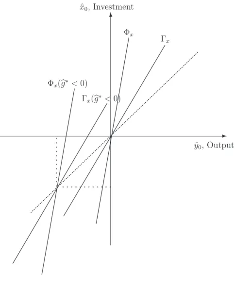
To understand how this mechanism works it useful to study the shock diagrammatically. Consider the simplest case, where the government imposes ∆B = 0. The export shock will shift both the ISBP and AD schedules, but the result will be a proportional change in output and investment, which is represented as a movement along a 45-degree line.
ˆ x0, Investment ˆ y0, Output 6 -Γx Φx Γx(bg∗ <0) Φx(bg∗ <0)
Figure 1: Fall in Exports
The proportional change in output and investment also occurs when private capital is un-restricted. However, without capital controls, the domestic interest rate is not affected by the shock. Here it is endogenous, and dependent on the source of the shock, but when a policy of ∆B = 0 is adopted the interest rate is independent of the change in exports, and this is why the capital mobility result is reproduced. Another way to interpret this result is in terms of the elasticities of the ISBP and AD schedules, defined in (29), which depend explicitly on ∆B. For output to over react; that is, for output to fall by more than the drop in exports, the following condition is required.
Φg∗+ Φx = φg
∗ +φx+ (φτ/ρτ)
1 + (φτ/ρτ)
>1 (30)
that characterize the AD schedule have to be larger than one. This result is attractive if one considers that the only additional equation in (29), versus the no capital controls case, is the LM equation, which forms part of the AD schedule. In fact, it is clear that the elasticity condition in (30) only requiresφg∗+φx >1. In other words, it is the sum of the elasticities
of output with respect to export demand and investment arising in the money market that determine whether output and investment mimic the no capital controls case with export shocks.24 The elasticity condition relates directly to government policy because it is possible to show, when ∆B <0,φg∗+φx >1, and when ∆B <0, the opposite holds. That is, when
the government chooses to force capital outflows, the sum of the elasticities of output with respect to export demand and investment in the money market are greater than one. In this case, output over reacts to the export shock.
The intuitive explanation for this result can understood from the reaction of the interest rate. Suppose the government chooses a policy of ∆B < 0. This implies that private agents are forced to save. To induce this type of behavior the domestic interest rate has to rise. But if this happens, consumption and investment fall. However, the drop in exports already lowers consumption and investment, as in the case without capital controls. Thus, the policy of ∆B < 0 exacerbates the impact of the shock. Likewise, if the government picks a policy of ∆B > 0, the interest rate will fall, shielding output from the change in exports. There is another important implication of this result, which can be understood from the diagram. Suppose the government forces private outflows of capital and output over reacts to the shock. In this case, investment will be more variable than output, and in terms of the diagram, we will always be below the 45-degree line. Thus, restrictions on capital flows may not only contribute to the variability of output when there are shocks to exports, they can also affect the relationship between output and investment.
Under the form of capital controls studied here the government acts directly as the financial intermediary because it holds a monopoly position in the supply of foreign bonds. Relative to the case where capital flows are unrestricted, this should offer some protection form to the domestic economy. However, this simple explanation turns out to be incorrect. One important implication of the analysis is that adopting capital controls in the face of export disturbances is a potentially bad idea in the sense that it may increase the variability of
24This requirement arises because the IS restriction, ρ
x+ρg∗ = 1, implies Γx−Γg∗ = 1 in the ISBP
output. At a minimum an important distinction can be drawn between the effects of inflow and outflow restrictions. If countries do, as Reinhart and Rogoff (2004) suggest, adopt dual exchange rate policies as a means to control the flow of private capital, this result also provides an interesting interpretation of the stylized fact that developing economies tend to have more volatile levels of GDP than their industrialized counterparts. Since one argument for capital controls is to insulate the economy from changes in foreign monetary conditions, even if this works, it opens up the possibility of large swings in domestic output as a result of export shocks.
B. Interest Rate Shocks
It is also often assumed that capital controls offer insulation from changes in the foreign interest rate. Without capital controls, changes in the foreign interest rate feed directly through to the domestic economy, and given this, the argument that capital controls offer a form of ‘insulation’ is relatively simple; by using a capital control the domestic nominal interest rate is no longer pegged to the foreign nominal interest rate. However, despite the use of capital controls, evidence of interest rate pass-through, such as that presented in Rogers and Miniane (2007), suggests higher foreign interest rates result in a higher domestic interest rates. Here, the same is true, and the pass-through has important implications because, when the flow of capital is unrestricted, a higher foreign interest rate has unambiguous implications for consumption, investment, and output - all fall. That is not the case when capital flows are restricted, as an increase in the foreign interest rate has two effects on consumption and output. There is a substitution effect away from current consumption which leads to lower current output. But there is also an off-setting or re-enforcing effect depending on the net foreign asset position of the economy because a higher interest rate makes the country either poorer or richer. Therefore, the reaction of consumption to changes in the interest rate is similar to the reaction of an individual - the income effect of the change implies that a borrower is hurt by the rise in interest rates, whilst a lender benefits. That is, consumption rises or falls with the shock, and this causes a potential ambiguity in the reaction of output.
Again, we can link the reaction of the economy to the shock back to the parameter that characterizes the AD schedule. In particular, it can be shown that the sign of Φi∗ depends
on the (endogenous) current period net foreign asset position of the economy; that is, Φi∗ ≡
Consider the expression for the change in output, as a result of a change in the foreign interest rate. b y0 = ΓxΦ ¡ ∆R−∆B¢−Γi∗Φx Γx−Φx bi∗ 0
The overall impact of the shock is ambiguous, but it is clear that a large part of this arises from the reaction of consumption. Again, it helps to consider a special case. When ∆R = ∆B output must fall when the foreign interest rate rises. Diagrammatically, only the ISBP shifts when ∆R= ∆B.
ˆ x0, Investment ˆ y0, Output Γx Φx 6 -Γx(bi0 >0)
Figure 2: Rise in the Foreign Interest Rate
It is clear from figure two that the reason output falls when the foreign interest rate rises and ∆R = ∆B is that investment falls. The potential ambiguity in changes in output therefore arise entirely from the income and substitution effects associated with consumption. It is also clear, in this case, that xb0 > yb0, and as ∆R changes, for a given policy choice over private capital flows, the relationship between consumption, investment, and output is affected.
This is an important result because it suggests that whilst capital controls can insulate an economy from changes in the foreign interest rate this insulation only works through aggregate demand. The governments holdings of foreign exchange also have implications for the behavior of output. In the context of previous studies, Flood and Marion (1982) use a stochastic Mundell-Fleming model and find that dual exchange rates provide full insulation from foreign interest rate shocks. This possibility fails here and the use of capital controls may have somewhat more severe consequences than previously thought.
One way to think about this result is through the non-linear NIBC, rewritten in terms of the domestic nominal interest rate,
¡ ∆R−∆B¢(1−1/τ0) = 1 X t=0 CAt/[(1 +i0)...(1 +it−1)] (31)
where (1 +i0)...(1 +it−1) ≡ 1 when t = 0. When τ0 = 1, the domestic and foreign rates of return are equalized, the left-hand side of this expression is zero, and discounting by the domestic of foreign nominal interest rate is equivalent, because there is no distortion in financial markets. However, when there is a capital control, the left-hand side of (31) is zero only when the economy is neither a net creditor nor debtor internationally. In response to the interest rate shock, τ0 changes, and the net foreign asset position of the economy affects wealth levels such that if, for example, the economy is a net creditor (∆R >
∆B), consumption rises, whilst investment falls. The wealth mechanism through which consumption rises does not operate when there are shocks to exports. That reserves matter for the macro consequences of interest rate shocks is particularly interesting. As Dollar and Kraay (2006) note, in China, reserve accumulation has largely mirrored the inflow of capital, which, relative to wealth, as reached around 4%. Thus, China’s zero net foreign asset position reflects debt flows and FDI that have been roughly balanced by the central banks accumulation of reserves. Given that China has a large number of capital controls in place, this points to the possibility that China could be insulated from any change in global interest rates.
5. Conclusion
This paper develops a general equilibrium model of a small open economy with physical capital, monopolistic competition and sticky prices to understand the implications of capital
controls. I show that the intertemporal equivalence between capital controls and dual exchange rates extends to a more general equivalence between the Mundell-Fleming and DGE approaches. The DGE economy has an upward-sloped balance-of-payments schedule and money demand plays an important role in determining the behavior of output, despite the exchange rate being fixed. As both of these features are a result of government policy, at first glance, the model appears to be much like the textbook Mundell-Fleming model. However, the economy differs from Mundell-Fleming in that budget constraints are imposed on individual behavior and also dictate how government reserves respond to external shocks. Some of the results contrast strongly to the standard logic which supposes that restrictions on capital flows help reduce output fluctuations in response to external shocks. If, as Reinhart and Rogoff (2004) suggest, countries have been using capital controls by imposing a financial exchange rate, the analysis points to an interesting explanation of why output in developing economies is more volatile - capital controls themselves are a source of instability.
References
Adams, C., Greenwood, J., 1985. Dual Exchange Rate Systems and Capital Controls:
An Investigation, Journal of International Economics 18, 43-63.
Aizenman, J., 1985. Adjustment to Monetary Policy and Devaluation under Two-Tier
and Fixed Exchange Rates,Journal of Development Economics 18, 153-169.
Alesina, A., Grilli, V., Milesi-Ferretti, G., 1993. The Political Economy of
Cap-ital Controls, in L. Leiderman, L., Razin, A. (eds.), Capital Mobility: New Perspectives, Cambridge University Press.
Calvo, G., Reinhart, C., and V´egh, 1995. Targeting the Real Exchange Rate: Theory
and Evidence,Journal of Development Economics 47, 97-133.
C´espedes, L., Chang, R., Velasco, A., 2004. Balance Sheets and Exchange Rate
Policy, American Economic Review 94, 1183-1193.
Chari, V, Kehoe, P, McGratten, E., 2002. Can Sticky Price Models Generate Volatile
and Persistent Real Exchange Rates?, Review of Economic Studies 69, 533-564.
Cook, D., Devereux, M., 2001. Capital Flows, Capital Controls and Exchange Rate
Policy, mimeo, HKUST.
Dollar, D., Kraay, A., 2006. Neither a Borrower nor a Lender: Does China’s Zero Net
Foreign Asset Position Make Sense?,Journal of Monetary Economics 53, 943-971.
Dornbusch, R., 1988. Exchange Rates and Inflation, MIT Press.
Fender, J., Yip, C., 2000. Tariffs and Exchange Rate Dynamics Redux, Journal of
International Money and Finance 19, 633-655.
Flood, R., Marion, N., 1982. The Transmission of Disturbances under Alternative
Exchange-Rate Regimes with Optimal Indexing,Quarterly Journal of Economics 97, 43-66.
Frenkel, J., Razin, A., 1986. The Limited Viability of Dual Exchange Rate Regimes,
NBER working paper 1902.
Guidotti, P., V´egh, C., 1992. Macroeconomic Interdependence under Capital Controls:
A Two-Country Model of Dual Exchange Rates, Journal of International Economics 32, 353-367.
Lahiri, A., Singh, R., V´egh, C., 2006. Segmented Asset Markets and Optimal Exchange Rate Regimes,Journal of International Economics (forthcoming).
Lane, P., Milesi-Ferretti, G., 2001. The External Wealth of Nations: Measures of
For-eign Assets and Liabilities for Industrial and Developing Countries,Journal of International Economics 55, 263-94.
Lane, P., Milesi-Ferretti, G., 2006. The External Wealth of Nations Mark II: Revised
and Extended Estimates of Foreign Assets and Liabilities, 1970-2004, CEPR Discussion Paper 5644.
Levy-Yeyati, E., Sturzenegger, F., 2005. Classifying Exchange Rate Regimes: Deeds
vs. Words,European Economic Review 49, 1603-1635.
Marion, N., 1981. Insulation Properties of a Two-Tier Exchange Market in a Portfolio
Balance Model,Economica 48, 61-70.
Miniane, J., 2004. A New Set of Measures on Capital Account Restrictions, IMF Staff
Papers 51, 276-308.
Miniane, J., Rogers, J., 2007. Capital Controls and the International Transmission of
U.S. Money Shocks, Journal of Money, Credit, and Banking (forthcoming).
Mendoza, E., 1991. Capital Controls and the Gains from Trade in a Business Cycle Model
of a Small Open Economy,IMF Staff Papers 38, 480-505.
Reinhart, C., Rogoff, K., 2004. The Modern History of Exchange Rate Arrangements:
A Reinterpretation, Quarterly Journal of Economics 119, 1-48.
Reinhart, C., Smith, T., 2002. Temporary Controls on Capital Inflows, Journal of
International Economics 57, 327-351.
Sachs, J., 1981. The Current Account and Macroeconomic Adjustment in the 1970’s,
Appendix
Here I derive the ISBP-AD representation of the economy with capital controls, given by equation (29). I start with the national budget constraint,
e£Rt+Bt−(Rt−1+Bt−1) ¡ 1 +i∗ t−1 ¢¤ = Ph,ty∗h,t−Pf,tyf,t = egt∗−(1−n) (Ωt+Ptxt)
where the intratemporal micro-demand conditions are imposed. I first make some simplifi-cations. Since R−1 and B−1 are given, I set them to zero, and since I consider permanent changes in exports, g∗
0 = g∗1 ≡ g∗. Both the NIBC and NBC need to hold with capital controls. These are, respectively,
(1−n) · ¡ Ω0+P x0 ¢ + Ω1 1 +i∗ 0 ¸ =eg∗ µ 1 + 1 1 +i∗ 0 ¶ and M0−D0 =eg∗−(1−n) ¡ Ω0+P x0 ¢ + ∆B
where M0 = e·∆R+D0 has been imposed. Using the consumption Euler condition the NIBC becomes, (1−n) · Ω0 µ 1 + β T0 ¶ +P x0 ¸ =eg∗ µ 1 + 1 1 +i∗ 0 ¶
In the current period output is demand constrained. Using the goods market equilibrium condition, (21), with the NIBC produces the IS equation.
y0Ph = n ³ 1 + 1 1+i∗ 0 ´ τ0 (1−n) (τ0+β) + 1 eg∗ + µ βn τ0+β ¶ P x0 (32)
Money demand needs to be consistent with the NBC, as in the main text. Combining this with the goods market equilibrium condition produces the LM equation,
y0Ph = n¡∆B+D0 ¢ aτe0+ 1−n +eg∗ µ aeτ0+ 1 aτe0+ 1−n ¶ +nP x0 µ aeτ0 aeτ0+ 1−n ¶ (33) whereτe0 ≡(1 +i∗0) [(1 +i∗0)−τ0]−1. To derive the BP equation, start with the future period goods market equilibrium condition. Since x1 = 0,
Substituting in the NIBC and the consumption Euler equation, thereby eliminating future consumption, y1Ph,1 = · nβ(2 +i∗ 0) (1−n) (τ0+β) + 1 ¸ eg∗− µ nβ(1 +i∗ 0) τ0+β ¶ P x0 From the factor demand and price setting conditions,
k1Q1Θ =y1Ph,1
where Θ ≡ θ/(θ−1)γ. From the households capital and consumption choices, Q1 =
P(1 +i∗
0)/τ0. Combining these conditions and eliminating y1Ph,1, which is endogenous, produces the BP equation.
P x0 ¡ =P k1 ¢ = eg∗ 1−n µ τ0 nβτ0+ Θ (τ0+β) ¶ · nβ µ 1 + 1 1 +i∗ 0 ¶ +(τ0+β) (1−n) 1 +i∗ 0 ¸ (34) Also note, the relative price of goods can be expressed using the following conditions;
¡ e/P¢ =q,¡e/Ph ¢ =q1/n, and ¡P /P h ¢ =q(1−n)/n.
I linearize the three conditions; (32), (33), and (34) around the no-shock equilibrium. IS:
b y0 =ρxbx0+ρττb0+ρg∗bg∗ −ρi∗bi∗0 (35) where, ρx ≡ q(1−n)/nx 0 y0 nβ τ0+β ;ρτ ≡ C0q(1−n)/n y0 nβ τ0+β ρg∗ = 1−ρx; ρi∗ ≡ i ∗ 0 (1 +i∗ 0)2 q1/ng∗ y0(1−n) nτ0 τ0+β
withρx ∈(0,1), becauseyPh =n(Ω +xP) +eg∗, and where all remaining terms on the right
hand side are positive. LM:
b y0 =φxxb0−φττb0+φg∗bg∗+φi∗bi∗0 (36) where, φx ≡ q(1−n)/nx 0 y0 na(1 +i∗ 0) a(1 +i∗ 0) + (1−n) [(1 +i∗0)−τ0] φτ ≡ C0q (1−n)/n y0 naτ0eτ0 a(1 +i∗ 0) + (1−n) [(1 +i∗0)−τ0] φg∗ ≡ qg ∗ y0 a(1 +i∗ 0) + [(1 +i∗0)−τ0] a(1 +i∗ 0) + (1−n) [(1 +i∗0)−τ0] φi∗ ≡ C0q (1−n)/n y0 aτ0i∗0/[(1 +i∗0)−τ0] a(1 +i∗ 0) + (1−n) [(1 +i∗0)−τ0]
with φx, φi∗ ∈(0,1) and φg∗,φτ >0. BP: b x0 =bg∗+λττb0+λi∗bi∗0 (37) where, λτ ≡ · τ0(1−n) nβ(2 +i∗ 0) + (τ0+β) (1−n) + Θβ nβτ0+ (τ0+β) Θ ¸ λi∗ ≡ i ∗ 0 1 +i∗ 0 · nβ+ (τ0+β) (1−n) nβ(2 +i∗ 0) + (τ0+β) (1−n) ¸
with λτ >0 and λi∗ ∈(0,1). Combine (35) and (37). ISBP:
b y0 = Γxbx0−Γg∗bg∗ + Γi∗bi∗0 (38) where, Γx≡ ρτ λτ +ρx; Γg∗ ≡ ρτ λτ −ρg∗; Γi∗ ≡λi∗ρτ λτ −ρi∗
whereρg∗ = 1−ρx implies Γx = 1 + Γg∗. Combine (35) and (36. AD:
b y0 = Φxxb0+ Φg∗gb∗+ Φi∗bi∗0 (39) where, Φx ≡ φx+ ρxρφττ 1 + φτ ρτ ; Φg∗ ≡ φg∗+ ρg∗φτ ρτ 1 + φτ ρτ ; Φi∗ ≡ φi∗−ρi∗φτ ρτ 1 + φτ ρτ
Equations (38) and (39) form (29) in the main text.
Now consider a permanent change in exports. The multiplier is,
b y0 = ¯ ¯ ¯ ¯ ¯ 1−Γx −Γx Φg∗ −Φx ¯ ¯ ¯ ¯ ¯ ¯ ¯ ¯ ¯ ¯ 1 −Γx 1 −Φx ¯ ¯ ¯ ¯ ¯ b g∗ = · (1−Γx) (−Φx) + ΓxΦg∗ Γx−Φx ¸ b g∗
First, note Γx >Φx > 0, and Γg∗ >0 ⇒Γx >1. Second, we can determine when by0 >bg∗
because, in this case, (1−Γx) (−Φx) + ΓxΦg∗ >Γx−Φx, or,
Φg∗+ Φx = φg∗ +ρg∗φτ ρτ 1 + φτ ρτ +φx+ ρxφτ ρτ 1 + φτ ρτ >1
Imposing ρg∗ = 1−ρx, ρxφτ ρτ +φx+ (1−ρx)φT ρτ +φg∗ > 1 + φτ ρτ φx+φg∗ > 1
which can be expressed as,
nq(1−n)/nx0aτe0+q1/ng∗(aeτ0+ 1)> y0[aeτ0 + (1−n)]
However, we also know the goods market equilibrium condition holds, so the previous con-dition reduces further, and only holds if ∆B+D0 <0. Suppose D0 = 0. Then; (outflows) ∆B < 0 =⇒ overreact; (private autarky) ∆B = 0 =⇒ equal change; (inflows) ∆B > 0 =⇒
under react. Likewise, ifyb0 >bg∗, it is also possible to show xb0 >by0.
Now consider a change in the foreign interest rate. The multiplier is,
b y0 = ¯ ¯ ¯ ¯ ¯ Γi∗ −Γx Φi∗ −Φx ¯ ¯ ¯ ¯ ¯ Γx−Φx b g∗ = · −Γi∗Φx+ Φi∗Γx Γx−Φx ¸ b g∗
Here, Φi∗ measures the consumption response to the shock, and its sign depends on the net
foreign asset position of the entire economy. To see this note, Φi∗ µ 1 + φτ ρτ ¶ = µ φi∗ φτ −ρi∗ ρτ ¶ φτ where, φi∗ φτ = i∗0 1 +i∗ 0 ;φi∗ φτ = i∗0 1 +i∗ 0 µ eg∗/(1 +i∗ 0) (1−n) Ω0 ¶ µ τ0 β ¶
Using these conditions with the NBC it can be shown that, Φi∗ = i ∗ 0φτ 1 +i∗ 0 µ 1 + φτ ρτ ¶−1µ τ0/β (1−n) Ω0 ¶ ¡ eR0−∆B ¢ ≡ Φ¡∆R−∆B¢