Spatial variability of maximum and minimum monthly
temperature in Spain during 1981-2010 evaluated by Correlation
Decay Distance (CDD).
Pena-Angulo D (1-2), Cortesi N (1-2), Brunetti M (3),
González-Hidalgo J.C. (1-2)
1. Department of Geography, University of Zaragoza, Spain, 50009 2. Instituto Universitario de Ciencias Ambientales (IUCA), Spain. 3. ISAC-CNR, Bologna
Author contact José Carlos González Hidalgo, [email protected] Manuscript
Click here to download Manuscript: Pena_texto_tac_V1.docx Click here to view linked References
1 2 3 4 5 6 7 8 9 10 11 12 13 14 15 16 17 18 19 20 21 22 23 24 25 26 27 28 29 30 31 32 33 34 35 36 37 38 39 40 41 42 43 44 45 46 47 48 49 50 51 52 53 54 55 56 57 58 59 60
Abstract
We present an analysis of spatial variability of monthly minimum and maximum temperatures in the conterminous land of Spain (Iberian Peninsula, IP), between 1981-2010, by using the Correlation Decay Distance function (CDD), with the aim of evaluating, at sub-regional level, the optimal threshold distance between neighbouring stations that makes the
network (in terms of stations’ density) well representative of the monitored region. To this
end, we calculated for 1981-2010 period the correlation matrix among monthly temperature series from AEMet (National Spanish Meteorological Agency) archives and analyzed the CDD.
In the conterminous land of Spain the distance at which couples of stations have a common variance in temperature (both maximum Tmax, and minimum Tmin) above the selected threshold (50%, r Pearson ~0.70) on average does not exceed 400 km, with relevant spatial and temporal differences. The spatial distribution of the CDD shows a clear coastland-to-inland gradient at annual, seasonal and monthly scale, with highest spatial variability along the coastland areas and lower variability inland. The highest spatial variability coincide particularly with coastland areas surrounded by mountain chains and suggests that the orography is one of the most driving factor causing higher interstation variability. Moreover, there are some differences between the behaviour of Tmax and Tmin, being Tmin spatially more homogeneous than Tmax, but its lower CDD values indicate that night-time temperature is more variable than diurnal one. The results suggest that in general local factors affects the spatial variability of monthly Tmin more than Tmax and then higher network density would be necessary to capture the higher spatial variability highlighted for Tmin respect to Tmax.
Key Words. Maximum and Minimum Temperature. Spatial Correlation. Variability. Spain. 1 2 3 4 5 6 7 8 9 10 11 12 13 14 15 16 17 18 19 20 21 22 23 24 25 26 27 28 29 30 31 32 33 34 35 36 37 38 39 40 41 42 43 44 45 46 47 48 49 50 51 52 53 54 55 56 57 58 59 60
1. Introduction
The research on climate change from the last century suggests that the most appropriate analyses for detecting any signal should be done using as dense as possible high quality dataset (Hansen and Lebedeff, 1987; Madden et al., 1993; Osborn and Hulme, 1997; New et al., 2000; Jones and Moberg, 2003; Caesar et al., 2006). High quality dense dataset also are demanded for climate models validation to detect possible effects of climate forcing, because “how well a model reproduces reality in a region with little data must be an open question” (Jones et al., 1997). Finally, high density database have proved to be increasingly important in the recent past, and they are likely to become even more important in the future, as decision support tools in a wide spectrum of fields such as, just to cite a few, energy, agriculture, engineering, hydrology, ecology and natural resource conservation (New et al., 2000).
The spatial coherence of meteorological variables is a well know problem particularly relevant when we are dealing with interpolation tasks (see Gandin, 1988; Eischeid et al., 1995; Jones and Mober, 2003; Shen et al., 2001; Raynaud et al., 2008). Gunst (1995) presented a review of spatial variability detection in climate elements and its application, from which emerged the correlation distance analyses as one of the most commonly used practice, generically named Correlation Decay Distance (CDD), Correlation Decay Lengths (CDL) or decorrelation length.
The CDD (recently revised by Pannekoucke et al., 2008) is defined as follows:
where r is the correlation between neighboring stations, x the distance between stations, and x0 the distance where the correlation r values fall below a defined threshold. In general this threshold is assumed to be (1/e) for large sample size data (Madden et al. 1993; Briffa and Jones, 1993; Jones and Briffa, 1996; Osborn and Hulme, 1997; New et al., 2000; Caesar et al., 2006; Hofstra and New, 2009), and represents the distance at which interstation correlation is no longer significant at the 95% level (i.e.: r ~0.36 for N ≥30). Greater values of CDD indicate that more distant stations retain a significant correlation and the spatial variability of the analyzed variable is low, and vice versa (Hofstra and New, 2006; Osborn and Hulme, 1997; Briffa and Jones, 1993). This spatial variability of correlation could be affected by geographical factors such as mountain barriers, land-ocean contact etc (Jones et al., 1997) which may drive some anisotropy behavior.
In general precipitation presents a stronger decrease of interstation correlation with distance (i.e. is has high spatial variability) than temperatures (New et al., 2000), however new observation tools, such as meteorological radars, provided an important step forward into the improvement of precipitation monitoring at the adequate spatial resolution. This is not true for temperatures, for which station networks still represent the most reliable source of information. Notwithstanding Hansen and Lebedeff (1987) have suggested that “before analyze a large-area temperature change from stations measurements, it is important to have a quantitative measure of the size of the surrounding area for which a given station´s data may provide a significant information of temperature change”. This preliminary step would help to avoid any bias when the irregular distribution of the available original stations were converted in a continuous field, such as a grid, (Jones and Moberg, 2003; Mitchell and Jones, 2005; Caesar et al. 2006; Hofstra and New, 2009), or when spatial variability in the original data is unknown. 1 2 3 4 5 6 7 8 9 10 11 12 13 14 15 16 17 18 19 20 21 22 23 24 25 26 27 28 29 30 31 32 33 34 35 36 37 38 39 40 41 42 43 44 45 46 47 48 49 50 51 52 53 54 55 56 57 58 59 60
The overall values of CDD for monthly temperatures, defined as the distance at which the selected common variance between couples of stations decrease below certain threshold, usually exceed hundreds of kilometers, and high differences have been highlighted in different latitudinal bands. At global scale, Hansen and Lebedeff (1987) found that the Pearson’s correlation coefficient fell below 0.5 (i.e.: r2<0.25) at station distance of about 1.200 km on average, being lower the distance at low latitudes than at high latitudes, “probably as a consequence of the dominance of mixing by large-scales eddies at high latitudes”. Different results were reported by Jones et al. (1997) who found higher values of CDD in tropical areas than in mean latitudes; they suggest a global mean value around 1500 km at which r<0.5, similar to those reported by Mann and Parker (1993), Madden et al. (1993), Caesar et al. (2006), Kim and North (1991), and Osborn and Hulme (1997). A global mean value of 1200 km was used by Mitchell and Jones (2005), following the study of New et al. (2000), for global database preparation.
We have found few studies analyzing CDD for Temperature data at regional scales, and they came from very sparse regions. In Europe Agusti et al. (2000) reported for 50% of common variance (i.e.; r~0,7), a general value of 400 km for annual mean temperature values; in the Alpine areas, Auer et al. (2005) reported decreasing distance from 900 km to 700 km for annual and seasonal-monthly values respectively for the same critical value, and in Italy Brunetti et al. (2006) suggested for monthly values distances of 400 km, suggesting that the decrease in common variance was higher for Tmax and Tmin than for the mean one. Different values have been reported in India (Srivastava et al., 2009) and Canada (Hopkinson et al., 2012), where Shen et al. (2001) found a threshold value of 200 km for the same critical value as before. In Spain, Frías et al. (2002) discussed regional temperature spatial anomalies pattern in winter but no data was given, and Staudt et al. (2007) quoted that the cross-correlation between anomalies usually exceed 0.5 even at distances of the order of 500 km.
It is accepted that annual CDD values are generally higher than seasonal or monthly (Briffa and Jones, 1993; Jones et al., 1997; New et al., 2000; Auer et al., 2005; Caesar et al., 2006; Hofstra and New, 2009). Also seasonal differences have been reported by Briffa and Jones (1993), New et al. (2000), Caesar et al., (2006) and Hofstra and New (2009), who suggested that summer spatial variability was higher than winter variability in mid-latitudes, while Jones et al (1997) suggested higher spatial variability in spring, and similar values of CDD for summer and winter; Srivastava et al. (2009) found in Indian monthly maximum temperature the lowest CDD (450 km) in February-March and June and the highest (1100 km) in August and Autumn months, while Hopkinson et al. (2012) have recently found in Canada the highest values of CDD for Tmax in spring and autumn.
In this study, we present an analysis of the spatial variability of temperature (maximum and minimum) in the conterminous land of Spain using CDD defined as the distance at which the common variance between stations decrease below 50% (i.e. Pearson r~0.7). The aim is to quantify, at sub-regional level, the spatial variability of maximum and minimum temperature (Tmax and Tmin) to identify the optimal threshold distance between neighbouring stations that should characterize an ideal network suitable to support climate studies. The results also highlight the leading factors in driving the spatial variability of temperatures at sub-regional scale in the Iberian Peninsula.
2. Data and Methods
In the present study we have used the monthly mean values of maximum (Tmax) and minimum (Tmin) temperature data from the original data archived at Spanish Meteorological Agency (AEMet). These archives hold information of temperature from more than 4000 stations. Original series include numerous gaps and cover different periods, so to avoid this
1 2 3 4 5 6 7 8 9 10 11 12 13 14 15 16 17 18 19 20 21 22 23 24 25 26 27 28 29 30 31 32 33 34 35 36 37 38 39 40 41 42 43 44 45 46 47 48 49 50 51 52 53 54 55 56 57 58 59 60
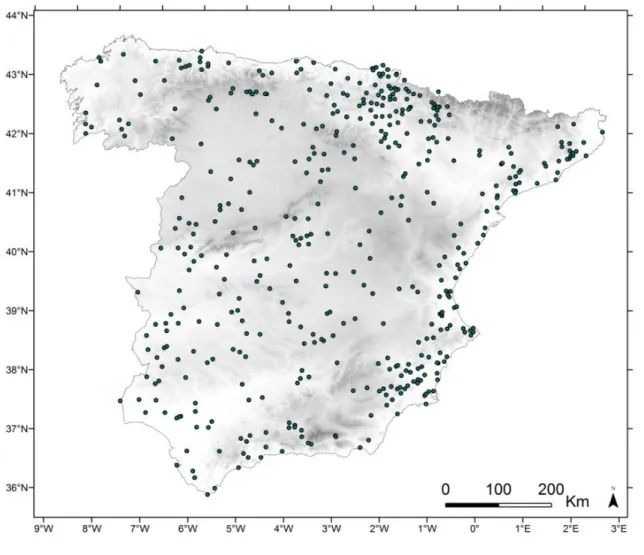
problem biases the results, CDD values were calculated using only the most complete series during 1981-2010 period; selected series had no more than 10% of monthly missing data, and quality control was applied to discard suspicious data and detect inhomogeneities in the frame of the HIDROCAES project. Thus we finally analyzed 459 and 454 series for Tmax and Tmin respectively. In Figure 1 we show the spatial distribution of stations.
The CDD analysis for Tmax and Tmin was performed calculating a correlation matrix at monthly scale. Correlation matrices were calculated using monthly anomalies data (difference between data and mean 1981-2010) to prevent the dominant effect of annual cycle in the CDD annual estimation. For each station, and time scale, the common variance r2
(using the square of Pearson’s correlation coefficient) was calculated between all neighbouring temperature series and the relation between r2 and distance was modelled according to the following equation (1):
(1)
being Log(rij2) the common variance between target (i) and neighbouring series (j), dij the
distance between them and b the slope of the ordinary least-squares linear regression model applied taking into account only the surrounding stations within a starting radius of 50 km and with a minimum of 5 stations required.
Such approach is similar to that of many other authors (Briffa and Jones, 1993; Jones and Briffa, 1996; Jones et al., 1997; Caesar et al., 2006; Srivastava et al., 2009), differing only in the introduction of the square of r in the first term of Eq. (1) and of the square root in the
second term, which were found to slightly improve the performance of the model for Spanish data. The high station density allows to increase the widely used threshold of r=0,50, and to define the CDD as the distance at which the common variance between target and neighbouring series is equal to 50%, i.e.: r2 ≥0,50 (r Pearson ~0,70) using Eq.(1).
Jones et al. (1997) stressed that a positive bias in the estimated CDD is introduced if all points with negative r are discarded before calculating the logarithm, and corrected the
problem adopting an iterative least-squares fit of its non-linear exponential model including all the negative r values. We choose a different solution that minimize the bias without changing the linear model: to avoid extrapolating the estimated CDD outside the upper bond of the regression interval (initially fixed at 50 km), if the estimated CDD is greater than 50 km, the starting radius was increased by 50 km and the CDD was re-calculated, until the estimated CDD was found to be lower than the radius within the model search for the stations (see Cortesi et al., 2013 b). In this way, points with negative r value are rarely included in the
model, because they are usually found at high distances (>400 km), while the majority of the regression models with variable distance stop before such length.
Finally, monthly, seasonal and annual CDD values were interpolated using the Ordinary Kriging with a spherical variogram over conterminous land of Spain, and converted on a regular 10 km2 grid (resolution similar to the mean distance between stations) to map the results. 2 ( )ij * ij Log r b d 1 2 3 4 5 6 7 8 9 10 11 12 13 14 15 16 17 18 19 20 21 22 23 24 25 26 27 28 29 30 31 32 33 34 35 36 37 38 39 40 41 42 43 44 45 46 47 48 49 50 51 52 53 54 55 56 57 58 59 60
3. Results
3.1. Annual mean values of CDD in Tmax and Tmin
The spatial pattern of annual CDD, calculated considering all monthly anomalies of Tmax and Tmin, is shown in Figure 2. Globally, CDD values are lower for Tmin than for Tmax, and the lowest values of CDD are found along coastland, while inland CDD values are higher. As a consequence Tmin is more variable than Tmax, even if it behaves more homogeneously because CDD presents stronger spatial gradients from coastland to inland in Tmax than in Tmin.
Tmax CDD annual values are about constant along North-East to South-West oriented bands (Figure 2), with lowest CDD values located at the south-eastern coastland sectors, where the values of CDD are lower than 100 km. The highest CDD values are found in extended areas of inland, with CDD ≥ 250 km, coinciding with the most flatty areas of Tagus, Guadiana, Duero and Ebro river catchments. In these areas it is not uncommon to found values of common variance >50% at distance over 300 km. Also for Tmin the lowest CDD values are found in coastland areas, with minimum values in the extreme coastland areas of south-east, but the area with CDD values lower than 150 km is more extended than for Tmax, and affect roughly half of the study area; moreover, the distribution of CDD values presents a latitudinal gradient from low CDD in southern areas to high CDD to the north.
3.2. Monthly mean values of CDD in Tmax and Tmin
The monthly analyses of Tmax and Tmin CDD show important differences (Figure 3). The main results are summarized as follows:
In general the lowest value of CDD, both for Tmax and Tmin, are found along the coastland of the Mediterranean fringe, while the highest CDD values are found in inland areas and in the extreme south-western coast. This fact is especially interesting because the southwestern coastland areas is open to the ocean air masses effects, while mountain barrier are parallel to the northern and south-eastern coastland.
CDD values are lower for Tmin than for Tmax in spring, summer and autumn months, i.e. nocturnal temperature has a higher spatial variability than diurnal one. During this period Tmax CDD shows a southeast to northwest spatial pattern in parallel bands, with higher values in south-east and northwest coastland areas, and lower to the inland and south-western coastland, while spatial distribution of Tmin CDD values presents a south to north gradient with lowest values to the south. In winter months, between November, December and January, CDD values are lower for Tmax than for Tmin, i.e. diurnal temperature is more variable than nocturnal one.
Because the lowest CDD values are found in summer in both Tmax and Tmin, maximum seasonal spatial variability in temperatures is found in summer.
The spatial pattern of CDD from February to October (except July-August) is similar in Tmax to the annual scale: minimum CDD values are located in south-east coastland areas while maximum ones are found to the inland and south-western coastland; it means that diurnal temperature spatial variability is higher in coastland areas than to the inland if the coastland areas are surrounded by mountain chain. To the south-east, the common variance of 50% usually is not retained far than 150 km, while in the inland areas it is found also for 1 2 3 4 5 6 7 8 9 10 11 12 13 14 15 16 17 18 19 20 21 22 23 24 25 26 27 28 29 30 31 32 33 34 35 36 37 38 39 40 41 42 43 44 45 46 47 48 49 50 51 52 53 54 55 56 57 58 59 60
distances higher than 300 km, similar value to those found in south-western coastland areas (see Figure 1 and 3) where no mountain barrier exist near the coast line.
On the contrary, Tmax during November, December and January and summer months (particularly July and August) shows the highest spatial variability. Over the most part of the area CDD is lower than 100 km. November-January is the only period in which CDD monthly values for Tmax are lower than for Tmin, with lowest CDD values located in coastland areas but also in the inland areas too. No clear spatial pattern has been found in winter CDD Tmax values.
During July and August summer months, the lowest CDD values of Tmax are located in coastland areas of north-west and south-east, with common variance of 50% at distances lower than 100 km; also in the inland areas the common variance of 50% is usually no achieved far than 200 km, being the highest values found on Ebro catchment. This monthly summer CDD spatial pattern is very similar to the annual one, but shifted toward lower values, and reflects high spatial variability in diurnal temperature.
Monthly analyses of Tmin reveal in general less inter-monthly differences, lower values than Tmax and a more homogeneous spatial behaviour. The lowest CDD values are usually located in the south-eastern coastland areas, and the spatial distribution of CDD generally presents a zonal shape except November, December, January and February. It is noteworthy to highlight the high CDD values for Tmin during this period when Tmax show low values. These findings reveal that from November to January the spatial variability is higher for diurnal temperature than for nocturnal one.
In Figure 4 we show same examples of monthly CDD for three selected stations from northern coastland (Bilbao), inland (Pantano Gasset, Ciudad Real) and southeastern coastland (Almería). Higher monthly spatial variability exists for CDD of Tmax than for Tmin. The CDD values for Tmin show a more regular annual cycle than Tmax do, with high CDD values in winter months and low values in summer months, with a latitudinal gradient from high monthly CDD to the north and lower to the south. This gradient is not so evident in Tmax CDD: in fact, for this variable there is a higher heterogeneity in monthly behavior.
3.2. The CDD in altitude
The most prominent result in the analyses of spatial variability of Tmax and Tmin in the Iberian Peninsula is the clear differentiation between coastland and inland. We have tried to analyze this different behavior taking into account that the Iberian Peninsula is a mountainous landscape with highly inland plateau (>500 m in altitude osl) surrounded by mountain chain of about 1000-3000 m. Meanwhile lowland areas are located in the coastland to the north, east and south, and also in the Ebro basin (north-east inland) and Guadalquivir basin (to the south-west), with altitudes lower than <500 m (see Figure 1).
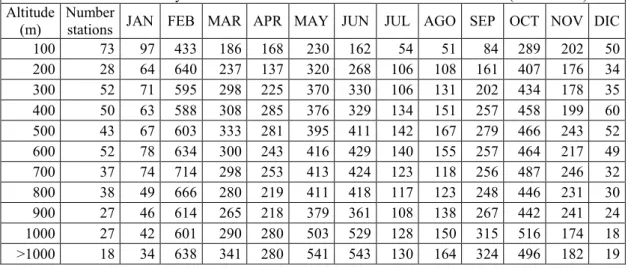
In Table 1 and 2 we show the monthly inter-stations CDD by altitudinal intervals, and Figure 5 show the altitudinal profile of the mean value of CDD. As a general rule the CDD increase with altitude for Tmax except in November, December and January. Maximum CDD values are achieved around 1000 m particularly in spring months. All these facts suggest that in altitude the Tmax spatial variability is lower than at low altitude, and then diurnal temperatures at low altitude (<200 m) are more affected by local conditions than upper levels. The CDD Tmin profiles are more homogeneous except for November-Dcember-January months. 1 2 3 4 5 6 7 8 9 10 11 12 13 14 15 16 17 18 19 20 21 22 23 24 25 26 27 28 29 30 31 32 33 34 35 36 37 38 39 40 41 42 43 44 45 46 47 48 49 50 51 52 53 54 55 56 57 58 59 60
Discussion and conclusions
Global analyses have suggested that CDD (using r=0,50 as threshold) for temperature usually are ≥1000 km (New et al. 2000, as example). Notwithstanding, regional studies reduces substantially the threshold distance of CDD to a few hundreds of km (Auer et al., 2005; Brunetti et al., 2006; Hopkinson et al. 2012) in agreement with our results in the Iberian Peninsula both for Tmax and Tmin.
In Spain we have found that interstation common variance decreases to values lower than 50% at distances almost always lower than 400 km. To our knowledge, such spatial variability of Tmax and Tmin has not been previously taken into account in past climate change studies in the Iberian Peninsula where the analysis is usually concerned only with differences in temperature trend (see in Bladé and Castro-Diez, 2010); as a result, the high spatial variability detected by mean of CDD in Tmax and Tmin in this paper suggests that monthly temperature trends in the Iberian Peninsula could be better expressed by using different regional temperature series of both Tmax and Tmin. Further analyses in progress, using high density database of temperatures, perhaps would be able to elucidate if spatial differences in temperature trends can be due or related to spatial variability of temperatures described by CDD, considering that trends in Tmax and Tmin could differ substantially. This fact could be of major importance as been highlighted by Christy et al. (2009) because observed trends of Tmax and Tmin can be promoted by different factors (see below).
At a global scale higher differences in CDD temperature values have been observed more pronounced along a meridional than zonal direction, but the latitudinal effect does not seem to be the main factor driving spatial distribution of temperature CDD values in the Iberian Peninsula. This is particularly true for Tmax, because in fact north and south-east coastland sectors show similar low CDD values (independently by latitude) in different months, suggesting that the distance from the sea coupled with close mountain barriers is one of the main driving factors in regulating the interstation Tmax correlation in the Iberian Peninsula. Meanwhile, there is a latitudinal gradient in CDD in Tmin, mainly from March to August.
The interstation correlation analyses shows that the lowest CDD values of annual mean temperatures are found during night (i.e. for Tmin), meaning that night-time temperature spatial variability is higher than diurnal-time temperature (i.e. Tmax). These findings suggest that the annual mean values of night-time temperature are more controlled by local factors (as land use from irrigation areas and latent heat fluxes) than diurnal temperatures, and probably is a consequence of complete changes in boundary layer dynamics, representing Tmax the greater daytime vertical connection to the deep atmosphere, whereas Tmin often reflects only a shallow layer thus the night temperature (i.e. Tmin) is highly dependent on local conditions (Christy et al., 2009; Hopkinson et al., 2012). Monthly analyses reveal that this annual behaviour is more complex and presents monthly variations that affect Tmax and Tmin (see Figure 5),.
Different papers have attributed spatial variability in CCD to geographical factors, such as orography (Irvine et al., 2011), the ocean-land contact (Hopkinson et al., 2012) and the atmospheric mechanism that governs climate along the seasons (Hansen and Lebedeff, 1987). In Spain the main mountain chains are oriented from west to east and north to south (see Figure 1), and isolate the northern and Mediterranean coastland areas, where low CDD values were found, from the inland areas, characterized by higher CDD values. This mountain orientation also affects the spatial Tmax CDD pattern, characterized (from March to October, see Figure 4) by south-east/north-west gradients, suggesting that the orography and the sea distance, between others, are the main driving factors; on the contrary, the south-western
1 2 3 4 5 6 7 8 9 10 11 12 13 14 15 16 17 18 19 20 21 22 23 24 25 26 27 28 29 30 31 32 33 34 35 36 37 38 39 40 41 42 43 44 45 46 47 48 49 50 51 52 53 54 55 56 57 58 59 60
coastland (where no mountain barrier exists) shows similar CDD values than inland ones. This fact is less evident in Tmin, where a meridional gradient is more frequent.
During the spring, summer and autumn months the CDD for Tmin is lower than Tmax: i.e. the spatial variability of night-time temperatures is higher than diurnal ones. These results are in agreement with Hopkinson et al. (2012) in Canada, Brunetti et al. (2006) in Italy, and also with New et al. (2000) and Caesar et al. (2006) at global scale for mid latitudes, suggesting more general geographical factors as main driving factors for Tmax and local for Tmin (see previous paragraph). Meanwhile, during November, December and January, the CDD of Tmax is lower than Tmin, and suggests that local factors could modify the spatial distribution of diurnal temperature values. A possible explanation could be the frequent foggy conditions characteristic of the inland catchments, enhanced by local topographical depressions, and under the anticyclonic atmospheric condition, which is the most frequent weather type in winter (Cortesi et al., 2013a). It means that in extended areas of the inland Iberian Peninsula winter Tmax is probably affected by local conditions, and diurnal temperatures suffer higher spatial variability than night-time in between November, December and January months varying CDD by altitude (Figure 5). Under this conditions the dynamic of diurnal mixing layer in extended areas could be reduced by temperature inversion as it usually occur in night time (Tmin); this diurnal inversion then could promote higher diurnal spatial variability. This fact does not extend during February when CDD Tmax values are higher than 200 km. We have no answer at present for that question, except the reduction of anticyclonic conditions between January to February around 20% during 1981-2010 (Cortesi et al. 2013a).
These findings suggest that spatial variability of Tmax and Tmin in the Iberian Peninsula is high and temporally varies. Then, a reasonable threshold distance for the selection of neighborhood stations in climate analyses should be evaluated according to the examined area and the period of the year. In any case, an average value of threshold distance of about 200 km should be considered as a limit value, lower than what previously accepted in bibliography. This variability also suggests that temperature trend in Spanish conterminous land should be evaluated separately for different sub-regional areas. Research in progress is focused on such objective.
To conclude, for many objectives and climate research tasks, as regional climate series construction, references series selection, grid interpolation etc., following the results of the present research the station selection in the Iberian Peninsula should be done cautiously, both to extrapolate the information down to a site location or to upscale it to a model grid box (Osborn and Hulme (1997).
Acknowledgments
Financial support given by Gobierno de España-FSE, Research Project CGL2011-27574-C02-01, and Gobierno Regional de Aragón DGA-FSE, and Grupo de Investigación Consolidado "Clima, Agua, Cambio Global y Sistemas Naturales" (BOA 69, 11-06-2007). Nicola Cortesi and Dhais Peña are PhD students, FPI Program, Gobierno de España. We give special thanks for his comments to Dr. S Vicente (IP-CSIC).
References
Agustí A, Thompson R, Livingstone DM (2000) Reconstruction temperature variations at high elevation lake sites in Europe during instrumental period. Verh. Internat. Verein. Limnol. 27: 479-483. 1 2 3 4 5 6 7 8 9 10 11 12 13 14 15 16 17 18 19 20 21 22 23 24 25 26 27 28 29 30 31 32 33 34 35 36 37 38 39 40 41 42 43 44 45 46 47 48 49 50 51 52 53 54 55 56 57 58 59 60
Auer I, Böhm R, Jurkovic A, et al (2005) A new instrumental precipitation dataset for greater Alpine region for the period 1800-2002. International Journal of Climatology 25: 139-166.
Bladé I, Castor-Díez Y (2010) Tendencias atmosféricas en la Península Ibérica durante el periodo instrumental en el contexto de la variabilidad natural. In: Perez F and Boscolo R (eds) Clima en España: pasado, presente y futuro. MedCLIVAR Spain, pp 25-42. Briffa KR, Jones PD (1993) Global surface air temperature variations over the twentieth
century. Part 2: implication for large scale paleoclimatic studies of the Holocene. Holocene 3: 77-88.
Brunetti M, Maugeri M, Monti F, Nanni T (2006) Temperature and precipitation variability in Italy in the last two centuries from homogenized instrumental time series. International Journal Climatology 26: 345-381.
Caesar J, Alexander L, Voss R (2006) Large-scale changes in observed daily maximum and minimum temperatures: creation and analysis of a new gridded data set. Journ. Geophysical Res. 111, DO5101.
Cortesi N, Trigo R, Gonzalez-Hidalgo JC, Ramos A (2013 a) Modelling monthly precipitation with circulation weather types for a dense network of stations over Iberia. Hydrology and Earth System Sciences 9: 665-678.
Cortesi N, Gonzalez-Hidalgo JC, Brunetti M, de Luis M (2013 b) Spatial variability of precipitation in Spain. Regional Environmental Change DOI: 10.1007/s10113-012-0402-6.
Eischeid JK, Baker CB, Karl TR, Díaz HF (1995) The quality control of long term climatological data using objective data analysis. Journal of Applied Meteorology 34: 2787-2795.
Frías MD, Rodríguez-Puebla C, Zubillaga J (2002) Variability study in winter maximum air temperature over the Iberian Peninsula: a comparison between observations and models. 2 Asamblea Hispano-Portuguesa de Geodesia y Geofísica, Valencia, Universidad Politécnica de Valencia.
Gandin LS (1988) Complex quality control of meteorological observations. Monthly Weather Review 116: 1137-1156.
Gunst R (1995) Estimating spatial correlations from spatial-temporal meteorological data. Journal of Climate 8: 2454-2470.
Hansen J, Lebedeff S (1987) Global trends of measured surface air temperature. Jr. Geophysical Research 92: 13345-13372.
Hofstra N, New M (2006) Spatial variability in correlation decay distance and influence on angular-distance weighting interpolation of daily precipitation over Europe. International Journal Climatology 29: 1872-1880.
Hopkinson RF, Hutchinson MF, McKenney DW, Milewska EJ, Papadopol P (2012) Optimizing input data for gridding climate normal for Canada). Jr. of Applied Meteorology and Climatology 51: 1508-1518.
Irvine EA, Gray SL, Methven J, Renfrew IA (2011) Forecast Impact of Targeted Observations: Sensitivity to Observation Error and Proximity to Steep Orography. Monthly Weather Review 139: 69-78.
Jones PD, Briffa KR (1996) What can the instrument records tell us about longer timescale paleoclimatic reconstructions?. In Bradley RS and Jouzel J (eds) Climate variations and forcing mechanisms of the last 2000 years. Springer, pp 625-644.
Jones PD, Osborn TJ, Briffa RK (1997) Estimating sampling errors in large-scale temperature averages. Journal of Climate 10: 2548-2568.
Jones PD, Moberg A (2003) hemispheric and large-scale surface air temperature variations: and extensive revision and uptodate to 2001. Journal of Climate 16: 206-223.
1 2 3 4 5 6 7 8 9 10 11 12 13 14 15 16 17 18 19 20 21 22 23 24 25 26 27 28 29 30 31 32 33 34 35 36 37 38 39 40 41 42 43 44 45 46 47 48 49 50 51 52 53 54 55 56 57 58 59 60
Kim KY, North GR (1991) Surface temperature fluctuations in a stochastic climate model. Jour. Geophysical Research 27: 405-430.
Madden RA, Shea DJ, Branstator GW, Ttribbia JJ, Weber RO (1993) The effects of imperfect spatial and temporal sampling on estimates of the global mean temperature: experiments with model data. Journal of Climate 6: 1057-1066.
Mann M, Park J (1993) Spatial correlation of interdecadal variation in global surface temperatures. Geophysical Res. Letter 20: 1055-1058.
Mitchell TD, Jones PD (2005) An improved method of constructing a database of monthly climate observations and associated high-resolution grids. International Journal of Climatology 25: 693-712.
New M, Hulme M, Jones P (2000) Representing twentieth-century space-time climate variability. Part II: development of 1901-1996 monthly grids of terrestrial surface climate. Journal of Climate 13: 2217-2238.
Osborn TJ, Hulme M (1997) Development of a relationship between station and grid-box rainday frequencies for climate model evaluation. Journal of Climate 10: 1885-1908. Pannekoucke O, Berre L, Desroziers G (2008) Background error correlation length-scale
estimates and their sampling statistics. Quaterly Journal of the Royal Meteorological Society 134: 497–511.
Raynaud L, Berre L, Desroziers G 2008. Spatial averaging of ensemble-based background-error variances. Quaterly Journal of the Royal Meteorological Society 134: 1003-1014. Shen SSP, Dzikowski P, Li GL, Griffith, D (2001) Interpolation of 1961-97 daily temperature
and precipitation data onto Alberta polygons of ecodistrict and soil landscapes of Canada. Journal of Applied Climatology 40: 2162-2177.
Srivastava AK, Rajeevan M, Kshirsagar SR (2009) Development of a high resolution daily gridded temperature data set (1969-2005) for the Indian region. Atmospheric Science Letter 10: 249-254.
Staudt M, Esteban-Parra MJ, Castro-Díez Y (2007) Homogeneization of long-term monthly Spanish temperature data. International Journal of Climatology 27: 1809-1823.
1 2 3 4 5 6 7 8 9 10 11 12 13 14 15 16 17 18 19 20 21 22 23 24 25 26 27 28 29 30 31 32 33 34 35 36 37 38 39 40 41 42 43 44 45 46 47 48 49 50 51 52 53 54 55 56 57 58 59 60
Figure 1. Spatial distribution of Tmax and Tmin series (1981-2010)
FigureFigure 2. Annual CDD mean value (in km) of Tmin (left) and Tmax (right) for r
2> 0,50.
Figure 4. Monthly variation of CDD (r
2> 0,50) in km for Tmin (top) and Tmax (bottom), at
three selected stations corresponding to north coastland (Bilbao, code 1082), inland
(Pantano Gasset, Ciudad Real code 4129) and south-eastern coastland (Almería, code
6325O).
0 100 200 300 400 500 600 700 800 CDD k m Tmin Bilbao Pantano Gasset Almeria 0 100 200 300 400 500 600 700 800 CDD k m TmaxFigure 5. Monthly variations of Tmax and Tmin mean CDD (in km) by altitude
January 0 200 400 600 800 1000 1200 0 100 200 300 400 500 600 700 800 Mean of CDD Al ti tu d e ( m ) February 0 200 400 600 800 1000 1200 0 100 200 300 400 500 600 700 800 Mean of CDD Al ti tu d e ( m ) March 0 200 400 600 800 1000 1200 0 100 200 300 400 500 600 700 800 Mean of CDD Al ti tu d e ( m ) April 0 200 400 600 800 1000 1200 0 100 200 300 400 500 600 700 800 Mean of CDD Al ti tu d e ( m ) May 0 200 400 600 800 1000 1200 0 100 200 300 400 500 600 700 800 Mean of CDD Al ti tu d e ( m ) June 0 200 400 600 800 1000 1200 0 100 200 300 400 500 600 700 800 Mean of CDD Al ti tu d e ( m ) July 0 200 400 600 800 1000 1200 0 100 200 300 400 500 600 700 800 Mean of CDD Al ti tu d e ( m ) August 0 200 400 600 800 1000 1200 0 100 200 300 400 500 600 700 800 Mean of CDD Al ti tu d e ( m ) Tmax Tmin September 0 200 400 600 800 1000 1200 0 100 200 300 400 500 600 700 800 Mean of CDD Al ti tu d e ( m ) October 0 200 400 600 800 1000 1200 0 100 200 300 400 500 600 700 800 Mean of CDD Al ti tu d e ( m ) November 0 200 400 600 800 1000 1200 0 100 200 300 400 500 600 700 800 Mean of CDD Al ti tu d e ( m ) December 0 200 400 600 800 1000 1200 0 100 200 300 400 500 600 700 800 Mean of CDD Al ti tu d e ( m )Table 1. CDD Tmax monthly altitudinal variation of inter station common variance (mean value) Altitude
(m) Number stations JAN FEB MAR APR MAY JUN JUL AGO SEP OCT NOV DIC
100 73 97 433 186 168 230 162 54 51 84 289 202 50 200 28 64 640 237 137 320 268 106 108 161 407 176 34 300 52 71 595 298 225 370 330 106 131 202 434 178 35 400 50 63 588 308 285 376 329 134 151 257 458 199 60 500 43 67 603 333 281 395 411 142 167 279 466 243 52 600 52 78 634 300 243 416 429 140 155 257 464 217 49 700 37 74 714 298 253 413 424 123 118 256 487 246 32 800 38 49 666 280 219 411 418 117 123 248 446 231 30 900 27 46 614 265 218 379 361 108 138 267 442 241 24 1000 27 42 601 290 280 503 529 128 150 315 516 174 18 >1000 18 34 638 341 280 541 543 130 164 324 496 182 19
Table 2. CDD Tmin monthly altitudinal variation of inter station common variance (mean value) Altitude
(m)
Number
stations JAN FEB MAR APR MAY JUN JUL AGO SEP OCT NOV DIC
100 74 311 333 80 86 161 90 61 61 98 169 353 274 200 28 284 269 106 75 204 71 63 41 93 169 379 301 300 50 273 313 109 72 179 92 70 53 103 120 329 358 400 49 339 310 153 113 196 123 95 77 124 138 359 348 500 43 319 321 131 118 190 117 81 78 133 122 374 347 600 51 341 285 121 73 160 91 64 52 109 106 336 328 700 37 331 326 103 126 204 111 56 56 131 151 396 355 800 37 310 270 81 108 181 100 43 65 115 112 340 301 900 27 442 405 115 118 191 88 56 90 152 133 421 390 1000 26 475 394 117 115 285 98 65 80 191 149 486 483 >1000 18 381 342 98 118 242 114 54 78 163 124 462 400 Table