Incumbent E¤ects and Partisan Alignment in Local Elections: a
Regression Discontinuity Analysis Using Italian Data
Emanuele Bracco
Lancaster University
Ben Lockwood
University of Warwick
Francesco Porcelli
University of Exeter
Michela Redoano
¤University of Warwick
First version: February 2011
This version: September 2014
Abstract
This paper provides a simple political agency model to explain the e¤ect of political alignment between di¤erent tiers of government on intergovernmental grants and election outcomes. Key fea-tures of the model are (i) rational voters interpret public good provision as a signal of incumbent competence, and (ii) realistically, grants are unobservable to voters. In this setting, the national government will use the grant as an instrument to manipulate the public good signal for the bene …t of aligned local incumbents. Then, aligned municipalities receive more grants, with this e¤ect being stronger before elections, and the probability that the aligned local incumbent is re-elected is higher. These predictions are tested using a regression discontinuity design on a new data-set on Italian mu-nicipalities. At a second empirical stage, the national grant to municipalities is instrumented with an alignment indicator, allowing estimation of a ‡ypaper e¤ect for Italian municipalities.
KEYWORDS: Fiscal Federalism, Political Competition, Accountability. JEL CLASSIFICATION: H2, H77, H87, D7
Address for correspondence; Department of Economics, Warwick University, Coventry, CV4 7 AL, United Kingdom. E-mail [email protected].
¤We would like to thank Andreas Hau‡er, Carlo Perroni and seminar participants at Warwick, Lancaster and Catholic
University in Milan, PET 2011, SIEP 2011, RES 2012, IIPF 2012 and SIE 2012 Conferences for helpful comments. Financial support from CAGE (Warwick) is gratefully acknowledged.
1
Introduction
This paper focuses on the implications for local public …nance, in particular, for intergovernmental grants, of three common features of …scal decentralization. The …rst is that there isvertical imbalancei.e. degree of decentralization in expenditures is signi …cantly higher than the degree of decentralization in tax revenue collection. For example, data from the World Bank Decentralization Database show that on average across over more than hundred countries and 29 years only over half of subnational expenditures are covered by subnational taxes. This vertical imbalance between …scal capacity and …scal needs is mostly covered by transfers from the central government.1 In some countries the allocation of these transfers is formula-based, while in others it is discretionary, giving central government potential scope for using grants for political goals.
A second common feature is that there are typically shared responsibilities between national and local governments in the provision of complex and important services such as health and education. For example, in the UK, the central government sets the school curriculum, and supervises exam marking, but local governments build and run schools, and hire teachers. Again in the education sector, in Italy the central government has sole responsibility for hiring teachers and deciding curricula, but school buildings are under the responsibility of provincial governments (for high schools) and municipal governments (for primary schools). At the same time regional governments are responsible for vocational training and bursaries. This second feature means that it is plausible that voters may have di¢culty assigning credit (or blame) for the quality of these services between a number of di¤erent levels of government.
A third feature is that local government is typicallyparty-political: that is, mayors and councillors have often party a¢liations, and the same parties operate at both the national and local level, so that the national and local incumbent parties may be aligned or non-aligned.
This paper studies how these last two features interact to shape the design of discretionary grants, local public expenditure and taxation, and local incumbency advantage. We take a principal-agent approach to modeling the relationship between voters and politicians, as in Alesina and Tabellini (2007). The local public good is produced from …scal resources (local tax revenue plus the grant) and also depends on local incumbent e¤ort and ability. Both local and national incumbents are quasi-benevolent; local incumbents care both about re-election and voter welfare, whereas national incumbents care about voter welfare, and the election of aligned local politicians. We can show that in this setting, the national government will give larger grants to aligned incumbents. This result is not new; Arulampalam et. al. (2009) have the same …nding in a distributive politics model where a national government can “buy" support from swing 1These …gures are based on own calculations on data from the World Bank Decentralization Indicators, available at http://www1.worldbank.org/publicsector/decentralization/ …scalindicators.htm. In particular we compute averages over 108 countries and 29 years (1972-2000) of the ratios between subnational tax Revenues and grants as a proportion of total subnational …scal capacity.
voters for aligned local incumbents. What is new is that our result is established in a micro-founded political agency model, where the mechanism at work can be identi …ed. Speci …cally, a higher grant raises local public good provision, and the latter signals a higher local incumbent ability to the electorate. This provides an incentive for the center to donate to districts with aligned incumbents. So, ours is a theory of intergovernmental grants as arising from the manipulation ofsignalsby the center, rather than by the o¤ering ofbribes by the center,in contrast to the standard political economy theory of grants (Cox and McCubbins(1986), Dixit and Londregan(1995, 1998))
Second, we develop a number of empirical predictions of our theory. The …rst one, is of course, an alignment e¤ect in grants. The second, which is new, is that a higher grant increases the probability of incumbent re-election, so that there is an alignment e¤ect on incumbency advantage. Third, we predict that the alignment e¤ect is stronger in election years than in non-election years. We also predict that conditional on grants, (i) local spending and taxes are independent of alignment, and (ii) there is a ‡ypaper e¤ect i.e. a one dollar increase in the grants has a bigger positive e¤ect on local government spending than does an equivalent rise in private income. These last two predictions suggest that the ‡ypaper e¤ect can be identi …ed by instrumenting grants by the alignment status of the local government. We then take these predictions to an original data-set on Italian mayoral elections and public …nance for the period 1998-2010.2 Italy constitutes a very good laboratory to test our hypotheses, as in Italy, grants from central government to municipalities have a large discretionary element, unlike most other OECD countries3. Our dataset includes almost 500 municipalities between 1998 and 2010, ruled by elected local governments, and around 25% of their current expenditure is funded by grants from the central and regional governments. There is no implicit or explicit formula for these grants, and each year a Budget Bill determines total grant for all municipalities, and the distribution of this total. Local taxes and fees cover most of the remaining 70% of local current expenditure. Local revenues are highly dependent on a property tax, ICI, which voters pay directly to their municipality. Moreover in the period covered by our data-set there have been three rounds of elections at the central level, while we observe local elections every year. The incumbent party at the central level has changed three times (in 2001, 2006 and 2008), and each year local elections were held in a number of municipalities. This gives us the variation in alignment that is needed to test our theory.
Our empirical strategy to identify the alignment e¤ects on grants and incumbent advantage uses a regression discontinuity design.4 Speci …cally, we compare municipalities where the elected mayor is just 2Data of Italian mayoral elections are taken for the period 1998-2008, therefore for the last two years we included in the sample only municipalities that did not have elections.
3Formula grants are extensively adopted, for example, in: Australia (82% at local level), Austria (98%), Denmark (97%), Portugal (85%), France (95%), United Kingdom. Discretionary ones are highly employed, for example, in Australia (at state level 90%), Czech Republic (88%), Turkey (100%). Data are our calculations from OECD Revenue Statistics, 2005 edition.
aligned with central governments with ones where the mayor isjustunaligned, where “just aligned” means that the mayor won the election with a small margin and that the mayor and the central government belong to the same party. Using this design, we …nd highly signi …cant alignment e¤ects that are robust across a number of di¤erent speci …cations, for both grants and incumbency. If a municipality is politically aligned with the party in power at the central level, it will be rewarded with on average, 40% more grants than unaligned municipalities. The probability that the aligned incumbent mayor (or his coalition) is re-elected in the election is, on average, 30% higher than in non-aligned ones. Moreover, this alignment e¤ect is stronger in the run-up to municipal elections than afterwards, in line with the theory.
The …rst empirical results tell us that alignment is potentially an appropriate instrument to use in testing the e¤ect of the grant on local expenditure and tax revenues. So, we test the e¤ect of alignment on local expenditure and tax revenues5, instrumenting the grant by an alignment dummy and also the margin of alignment. The over-identi …cation tests are passed, indicating that the instruments are valid and thus that alignment has no e¤ect on local expenditure, independently of the grant. The IV estimates indicate the presence of a ‡ypaper e¤ect. First, public spending increases by about 0.4 Euros per capita for each Euro increase in grants. On the other hand, a Euro increase in private income has a negligible e¤ect on public spending. So, the overall ‡ypaper e¤ect is around 0.4, in line with the results surveyed in Inman(2008).
The paper is organized as follows. The next section discusses the related literature. Section 3 intro-duces the theoretical framework, and Section 4 presents the main theoretical results. Section 5 presents some background information on Italy, data description and the econometric strategy. Section 6 discusses the main empirical results on transfers, and Section 7 is devoted to the ‡ypaper e¤ect. Section 8 tests the alignment e¤ect on incumbency, and Section 9 concludes.
2
Related Literature
Our work speaks to at least four related literatures. First, on the theoretical side, our paper develops a new political economy theory of intergovernmental transfers based on a principal-agent model of multi-level government. This extends the existing literature in two ways. First, there is now a huge literature on political agency (summarized in for example, Persson and Tabellini (2000), Besley (2006)), which stresses the role of elections in screening and monitoring politicians. However, this literature focusses on one level of government, and has hardly considered intergovernmental grants. One exception is Brollo between …scal choices and the ideological characteristics of its voters—to identify the alignment e¤ect on tax setting, grant allocation and public spending. A similar approach, in the context of grant allocation only, has been used in independent works by Brollo and Nannicini (2012) and Migueis (2013).
5In the Online Appendix we propose two alternative exercise, where the dependent variable is in turn (i) municipality expenditure net of (national and regional) grants, which corresponds to the sum of local taxes and fees, (ii) the total amount of public expenditures. The results for the estimation of the ‡ypaper e¤ect are very similar and around 40%
et. al. (2013), which shows how higher grants from central governments can have negative e¤ects on the behavior of lower-level governments in that the higher the transfer, the greater the rent taken by the lower-level incumbent, and when entry of incumbents is endogenized, the less good is incumbent quality. However, in that paper, grants are treated as exogenous6. Our theoretical contribution is to endogenize the grant in a setting very similar to Brollo et. al. (2013). So, this paper is the …rst, to our knowledge, to study intergovernmental grants in an agency framework.
Our approach is also in contrast to a “distributive politics" theory of intergovernmental grants due originally to Lindbeck and Weibull (1987), Dixit and Londregan (1995), and extended to a …scal federalism setting more recently by Dixit and Londregan (1998) and Arulampalam et. al. (2009)7. This literature takes a Downsian view; parties can pre-commit to intergovernmental transfers prior to the election, and these transfers are observable by voters, both strong assumptions. In Dixit and Londregan (1998), national parties choose intergovernmental transfers to maximize their vote share in the national election, taking into account any redistribution of these funds amongst voter groups by state governments. They …nd that the transfer from the center to a given state will be higher, the greater the average “clout" of voting groups in that state, where “clout" depends on the relative number of “swing" voters in that group, and how cheap those votes are to buy (the weight that voters in the group put on consumption relative to ideology).
Arulampalam et.al. (2009) modify the Dixit-Londregan set-up to allow transfers from national gov-ernment to impactdirectlyon voters’ incomes, and assume that national governments do not contest an election, but rather design grants to maximize the vote share of the aligned local candidates. Moreover, they assume that if the local and national incumbents are not aligned, the “goodwill" or utility incre-ment generated by the grant is shared between the local incumbent and challenger (the latter being by de …nition, aligned with the national incumbent, as there are only two parties). Speci …cally, it is assumed that the local incumbent gets a share of the goodwill, and local challenger 1¡= The qualitative predictions of the theory depend crucially whether this share is greater than one half. This is simply taken as exogenous in their theory, and indeed cannot be meaningfully endogenized in their model. One contribution of our theoretical model is that it e¤ectively endogenizes ; see Section 4 below for more discussion.
On the empirical side, there are several related literatures. First, there is the literature on political alignment e¤ects on intergovernmental grants. There are a number of papers that establish, for various countries, that political alignment with the center generates higher levels of discretionary grant to the 6Bordignon, Gamalerio and Turati (2013) extend Brollo et. al. (2013) to allow for two “quality" dimensions of politicians. Richer municipalities (with larger tax bases) are more likely to attract “productive" rather than “rent seeking" politicians. In their paper, rather than grants, the exogenous variation is from the 1999 reform in Italy that gave municipalities the power to set a surcharge on the income tax.
local government, for example, Levitt and Snyder (1995) and Larcinese, Rizzo and Testa (2006) for the US, Solé-Ollé and Sorribas-Navarro (2008) for Spain, Arulampalam et. al. (2009) for India, Case (2001) for Albania, Rodden and Wilkinson (2004) for India, Brollo and Nannicini (2012) for Brazil, Migueis (2013) for Portugal. In particular, our theoretical …nding that alignment e¤ects are stronger in election years is consistent with Brollo and Nannicini (2012), who estimate the alignment e¤ect on per capita average infrastructure transfers from the federal government to municipalities in the last two years of the mayoral term and in the …rst two years of the mayoral term. They …nd that aligned municipalities signi …cantly receive more grants than unaligned one only in the last two years of the term.
Second, there is a large literature on incumbency advantage. In particular, several recent papers use a regression discontinuity design in order to estimate the advantage of incumbency in elections, relying on the fact that when the electoral race is very tight, the identity of the winning party is likely to be determined by pure chance. The main contributions include Lee (2001, 2008), Lee, Moretti and Butler (2004) and Ferreira and Gyourko (2009). The common …nding is that an incumbent policy maker enjoys a considerable advantage in winning elections.8 Our approach di¤ers from the above because we are not attempting to estimate the incumbent e¤ect as such, but we estimate the e¤ect of alignment on incumbency, i.e. we estimate whether being just aligned with the central government increases an incumbent mayor’s chance of being re-elected compared with a just unaligned mayor.
Third, our paper also relates to the large empirical literature on the ‡ypaper e¤ect (for surveys, see Hamilton (1983) and Inman (2008)). One of the main problems faced by this literature is that intergovernmental grants may be endogenous, and thus unbiased estimates of the ‡ypaper e¤ect require either (i) identi …cation of truly exogenous changes in intergovernmental grants as in Dahlberg et al. (2008), or (ii) appropriate instruments for grants, as in Knight (2002). Our work is a contribution to the second strand of the literature; we are the …rst, to our knowledge, to use alignment as an instrument to estimate the ‡ypaper e¤ect.
Finally our paper is related to Bracco and Brugnoli (2012) and Cio¢, Messina and Tommasino (2012); they both analyze Italian local public …nance data to investigate the e¤ect of political competition on policies. Bracco and Brugnoli (2012) focus on the e¤ect mayoral electoral system on grant allocation and …nds that plurality elected mayors received less grants than colleagues elected under dual ballot system. Cio¢, Messina and Tommasino (2012) …nd evidence of a political cycle for local capital expenditures in those municipalities where the mayors are not politically aligned with the central government coalition.
8For example Ferreira and Gyourko (2009) …nd that, in the US, Democratic mayors who barely win an election have about a 66% chance of winning the next election.
3
A Theoretical Framework
3.1
The Environment
In a country there are two tiers of government: a central government, and l= 1> ==qlocal jurisdictions, also referred to as municipalities. There are two partiesO andU, which operate both at the central and local level. Without loss of generality, we assume that party O is ruling at the central level and in a subsetPD of local authorities, while the complementary subset of municipalities PQ is ruled by party U. The subscripts D and Q indicate that left-wing localities are aligned with the central government, while right-wing ones are non-aligned.
In each of two periodsw= 1>2> the incumbent mayor in municipality lproduces a local public good via the following production function
jlw=I(ulw) exp(hlw+dlw)> ulw=lw+Wlw (1) wherehlw> dlware incumbent’s e¤ort and ability levels, lwis local tax revenue (from a property or income tax) andWlwis a transfer from the central government. So,ulwis total …scal resources of the municipality, and is also equal to public expenditure. Also, we assume thatI(ulw) is non-negative, increasing inulw, and concave. Then, under these assumptions,jlw is non-negative.
Finally, the incumbent abilities dlw are determined as follows. First, the initial incumbent’s ability, dl1 is drawn from a distribution with mean zero, where the distribution is common knowledge between voters and the incumbent. If the initial incumbent retains o¢ce, his ability is the same in the second period i.e. dl2 =dl1= If he loses o¢ce, dl2 =df>l> where dfl is the challenger’s ability, drawn from the same distribution asdl1=
The order of events is as follows. In period 1, each incumbent mayor chooses hl1> l1> l= 1> = = = > q, and the national government choosesWl1> l= 1> = = = > q=. Then,jl1is determined via (1). Having observed jl1> l1 but not hl1> Wl1> the voters in region l vote in municipal elections for the incumbent or the challenger. The winners take o¢ce in period 2 and choose hl2> l2> l= 1> = = = > q. The national incumbent does not face an election and retains o¢ce, and choosesWl2> l= 1> = = = > qin period 2.
3.2
Payo¤s
In each municipalityl>there are a large number (a continuum of measure 1) of identical voters who have utility
x(jlw> flw) = lnjlw+flw (2) where flw is consumption of a private good. The private budget constraint of voter m in municipalityl at timewisflw=pm¡g(lw)where pm is private income>andg(lw)is the cost to the household of tax
revenue lw== We assume g(0) = 0> g0> g00 A 0, g() A > A 0> so that g captures the sum of loss of income and any of deadweight losses and compliance costs of taxation. This speci …cation is standard in the public …nance literature (e.g. Bolton and Roland (1997)).
Substituting the budget constraint into (2), and ignoringpm, we get a voter payo¤ over government policy oflnjlw¡g(lw). Moreover, following Dixit and Londregan (1998), voter y in municipality l has an ideological preference for the incumbent, measured negatively by[l=So, votery’s overall payo¤ is
lnjlw¡g(lw)¡[l (3)
We assume [l is distributed independently across voters and uniformly on [¡1@(2l)> 1@(2l)], with l inversely measuring the dispersion of ideological preferences in municipality l. So, l measures the strength of swing voting i.e. the sensitivity of voting choices to performance in o¢ce in municipality l.
The incumbent municipal politician is quasi-benevolent, i.e. cares about voter utility fromjlw> lw>but also dislikes e¤ort and values the probability of winning the election slw:
(lnjlw¡g(lw))¡#(hlw) +slwYlw> A0 (4) Here, is the weight on voter welfare, and Ylw is the continuation value of o¢ce for the incumbent, calculated at the point when policy is chosen at timew=In period2>by de …nition,sl2´Ylw´0;it can be shown (see the online Appendix) thatYl1=Y for all municipalities, andsl1 is determined as described below. Here,#(=)is a twice di¤erentiable, strictly increasing and strictly convex cost of e¤ort. We assume, without loss of generality, that Y = 1>so the re-election incentive is measured solely bysl1=Overall, (4) is quite a standard objective for the politician (see for example Besley (2006)).
The incumbent national politician is similarly quasi-benevolent, and also (as in Arulampalam et al. (2009)) cares about the payo¤s of incumbents in aligned jurisdictions, and challengers in non-aligned jurisdictions. So, his payo¤ is
X l2PD slw+ X l2PQ (1¡slw) + X l2P (lnjlw¡g(lw))¡ X l2P Wlw
where the cost of providing Wlw to a municipality l is normalized to unity. For simplicity, we assume a discount factor of one for all agents.
3.3
Discussion
The basic structure of the model is very similar to that of Brollo et al.(2013). The main di¤erences are twofold. First, the details of the public good production function and voter utility function are somewhat di¤erent, and second, more importantly, we endogenize the transfer Wl from central government. Note
that a crucial assumption is thatWlis not observed by the voter at the time of voting; without this, grants could not be used to signal. We believe that the assumption that Wl is not observed is very realistic; voters typically do not understand the complex rules governing formula grants, much less understand how discretionary grants are allocated. Finally, note that the assumption that the incumbent does not know his own ability at the beginning of his term of o¢ce is a widely made one in the literature on political principal-agent models (e.g. Persson and Tabellini(2000), Alesina and Tabellini(2007)); it keeps the analysis tractable while allowing the incumbent to signal his ability via higher public expenditure in equilibrium.
4
Theoretical Results
We solve the model backwards. In the second period, voter payo¤s are increasing in incumbent ability. In fact, as shown in the online Appendix, incumbents of all abilities choose the same levels of tax and e¤ort in the second period, so that the di¤erence in second period voter payo¤s over government policy between incumbents with abilitiesd> d0is justd¡d0=So, because incumbent ability is persistent, the voter
inlwishes to re-elect the incumbent only if the di¤erence between his expected …rst-period ability dh l1> and zero, the expected ability of the challenger, is higher than the voter’s ideological preference for the challenger, measured by[l=So, the voter will re-elect the incumbent if
dhl1¸[l (5)
From now on, we drop time subscripts, as all relevant variables are …rst-period. So, we see from (5) that the probability of the incumbent winning,sl> is generally
sl= Pr ([l·∙dhl) = 0=5 +ldhl (6) How isdh
l determined? We can assume without loss of generality that the voter makes his inference aboutdl by observing his utility from public good provision, which is
lnjl=i(l+Wl) +hl+dl> i= lnI (7) Note that by the assumptions on I> i is strictly increasing and concave.9 Then, if the voter expects e¤ort and the transfer to be at levelshh
l> Wlh>but observeslnjl>his inferred value of dhl must satisfy lnjl=i(l+Wlh) +hhl+dhl (8) 9This functional form implies that e¤ort and tax revenue are independent in the sense that C2lnj
C Ch = 0. If the two inputs > hare complements i.e. this cross-partial is strictly positive, Propositions 1, 3 and 4 would still hold. Proposition 2 instead would not, as—conditional on grants—aligned mayor would exert less e¤ort and levy lower taxes.
Then, combining (7), (8), we get
dhl =i(l+Wl) +hl¡i(l+Wlh)¡hhl +dl (9) That is, voter expectations are rational, up to any error in forecastingWl> hl=
The incumbent politician in l perceives his probability of victory to be the expectation of sl with respect todl=Combining (6),(9), we see that this is
shl = 0=5 +l(i(l+Wl) +hl¡i(l+Wlh)¡hhl) So, local governmentlchoosesl> hl to maximize
(i(l+Wl) +hl¡g(l))¡#(hl) + 0=5 +lshl takingWl> Wlh> hhl as given. The …rst-order conditions with respect tol> hl are:
+l=#0(hl)> i0(l+Wl) +l(i0(l+Wl)¡i0(l+Wlh)) =g0(l) (10) respectively. In equilibrium, expectations are rational, i.e. Wh
l =Wl> hhl =hl=So, (10) reduces to
+l=#0(hl)> i0(l+Wl) =g0(l) (11) The national government choosesWl to maximize
X l2PD lshl¡ X l2PQ lshl + X l2P (i(l+Wl) + hl¡g(l))¡ X l2P Wl
takingl> hl> Wlh> hhl as given. By the same argument, at equilibrium, the …rst-order conditions with respect toWl are
(+l)i0(l+Wl) = 1> l2PD (12) (¡l)i0(l+Wl) = 1> l2PQ (13) Collectively, these …rst-order conditions characterize any Nash equilibrium to the game between the central government and theqmunicipalities. From these …rst-order conditions, we can then establish the following results, all of which are proved in the Online Appendix.
Proposition 1. Alignment e¤ects on grants.If lis aligned, and m is non-aligned, thenWlA Wm= The intuition is as follows. First, national government has a baseline incentive to give transfers, because it cares about voter welfare. This is captured by the terms i0 in (12)-(13). In addition, the national government perceives that by raisingWl>there will be an unanticipated (by the voter) increase in
jl>and the incumbent will get the credit for this, raising the re-election probability sl= So, the national government will want to give more to aligned districts, and less to non-aligned ones. This is captured by the termli0 in (12), and¡
li0 in (13).
We can now compare our results to Arulampalam et. al. (2009). They assume that with alignment, the “goodwill" or utility increase for the voter generated by the grant is all captured by the local incumbent, but with non-alignment, it is shared between the local incumbent and challenger in exogenous shares> 1¡ respectively. Their Proposition 1, one of their main results, states that aligned incumbents get higher grants, independently of voter responsivenessl when the share of credit going to the challenger, ? 0=5> because when this holds, a grant to a non-aligned municipality unambiguously bene …ts the incumbent. In our micro-founded approach, building on well-known political economy models, we see that the non-aligned incumbent gets all the credit i.e. = 1=
Finally, note that Proposition 1 is a result for election years. By contrast, in the second period of the model, there are no alignment e¤ects i.e. transfers to aligned and non-aligned municipalities are the same. So, generally, our empirical prediction is that alignment e¤ects will be stronger in election years. The absence of an alignment e¤ect in non-election years is an artefact of the simplicity of the model and such an e¤ect could easily be introduced in a number of ways e.g. by supposing that the national government cares more about voter welfare in the aligned municipalities.
The second result says that alignment e¤ects on local taxes and spending only work through transfers. Proposition 2. No conditional alignment e¤ect on local taxes and spending. Conditional on transfers, local tax revenue and spending u=+W are independent of alignment.
The proof of this is obvious from (11). Writing the relevant conditions out in full, for any municipality l>we have:
i0(l+Wl) =g0(l) (14)
So,l is independent ofhl, which does depend directly on alignment= It then follows directly from (14) that tax revenue and expenditure only depend on alignment via transfers. We can now be more precise about how transfers a¤ect local taxes and spending:
Proposition 3.E¤ect of Transfers on local taxes and expenditure. A given increase in transfers will reduce taxes by
g gW =¡
iuu iuu¡g00
A¡1
and thus increase expenditures by
gu gW = 1¡
iuu iuu¡g00
A0
The intuition for this result is that as the transferW rises, the marginal deadweight loss of taxation falls, encouraging the municipality to raise more revenue overall, and thus does not fall one-for-one
withW=
This result leads to a prediction about the ‡ypaper e¤ect in our model. The ‡ypaper e¤ect is usually understood to be the stylized fact that grants have a bigger positive e¤ect on local government spending than does an equivalent rise in private income (Inman(2008)). In our setting, households preferences are linear in income (see (2)), so there is no private income e¤ect on government spending. However, we see from Proposition 3 that gWgu A 0> so our model predicts a ‡ypaper e¤ect of transfers. Moreover, these results suggest a way of identifying the ‡ypaper e¤ect via the use of alignment as an instrument, as discussed in Section 8 below.
Finally, we ask how the alignment e¤ect described in Proposition 1 impacts upon the fortunes of the incumbent in an election. We have seen that higher transfers from the center lead to greater public good provision, and one might expect that might help the incumbent win the election. It turns out that if all voters are fully rational, that is not the case; rational voters “see through" the higher jlw because they rationally anticipate that aligned incumbents get higher transfers.
However, it seems implausible that all voters behave like that; after all, the retrospective voting literature demonstrates empirically that good performance is rewarded (see for example Fiorina (1978) and Wolfers (2002)). This can be formalized in our model by assuming that there is a fraction 1¡ of the voters who are “naive retrospective" i.e. they are more likely to re-elect the incumbent if they see thatjl1 was higher (or equivalently, they received a higher utilitylnjl1¡g(l1)inw= 1). This can be contrasted with the “sophisticated retrospective" behavior of the fully rational voters in our model, who are more likely to re-elect the incumbent if they believe that dl was higher.10 Assume in particular that naive retrospective voter y votes for the incumbent if lnjl1¡g(l1)¸[l, where[l is distributed uniformly on[¡1@(2l)>1@(2l)], as for the rational voters. It is then straightforward to show that: Proposition 4. Alignment e¤ect on re-election probabilities. Assume that municipality l is aligned, andmis not. If some fraction A0of voters are naive retrospective, andl¸m>the incumbent is more likely to be re-elected inlthan in m.
The intuition is simply that when voters are weakly more responsive in the aligned jurisdiction (l¸m), alignment weakly increases e¤ort and strictly increases expenditure on the public good, thus increasing the level of the public good itself, and this increases the attractiveness of the incumbent for the naive retrospective voters.
1 0A similar result might be obtained with a multi-period model with solely forward-looking voters. In such a model all voters would be more likely to vote for the aligned incumbent, as long as aligned jurisdictions kept on o¤ering more public good for less tax. Nevertheless, the model would be substantially more complicated than the current one, as one would need to include further assumptions as to what extent voters are forward looking, how much “memory” the serially-correlated abilitydlw has; it would also require the formalization of upper-tier elections.
5
Empirical Analysis
5.1
Background Information on Italy
In this section we present some relevant background information on the Italian electoral system and local public …nance.
5.1.1 Tiers of governments, elections and parties
Italy is a unitary parliamentary republic ruled by a central government with three sub-national levels: regions (regioni), provinces (province), and municipalities (comuni); the latter are the subject of our analysis. Comuni are ruled by a city council (consiglio comunale), and an executive committee (giunta), headed by an elected mayor (sindaco). Mayors are in charge of appointing the members of the executive committee (giunta),to which tasks are delegated, including powers on land management and environment (water, sewage, public hygiene), local transport, local police, culture and recreation, education (nursery schools, complementary education services such as transport and meal service). Mayors also have some discretionary powers on how much …scal revenue to raise.
Following a political reform that took place in 1992, mayors are directly elected for …ve-year terms11 and are subject to a two-term limit. Mayors and city council are elected together, with di¤erent rules ap-plying to municipalities below or above the 15,000-inhabitant threshold (from now on referred to assmall and large municipalities), according to the latest available census data. Mayors of small municipalities are elected by …rst-past-the-post, while mayors of large municipalities are elected by runo¤. This means that if no mayoral candidate obtains an absolute majority, voters vote again on just two candidates, the winner and the runner-up of the …rst round.
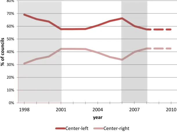
Generally speaking, in our sample period both at the local and at the national level, the political system was dominated by two large electoral cartels, the center-right and the center-left. At the national level, the center-right coalition ruled Italy from 2001 to 2006 and again from 2008 to 2011. The center-left coalition, going from Communist parties to left-leaning Christian Democrats, ruled instead from 1996 to 2001, and then again from 2006 until 2008.
However, the two-tier electoral system means that the electoral cartels are less in‡uential in the smaller municipalities. Speci …cally, in smaller municipalities, because of the …rst-past-the post system, there is less incentive for small parties and independents to form coalitions to support a single candidate, whereas in the larger municipalities, there is a strong incentive to …eld a candidate who can win at the …rst round. Coalitions, when they form, are usually easy to classify as left or right, because they usually a¢liate with a national party. This means that the party of both the winning mayor and the other contestants in the
election is much easier to classify as “left" or “right" in large municipalities.
This is shown in Table 1, which shows the type of party (or coalition of parties) of the winning mayors in all municipal elections from 1998 to 2008, using o¢cial data published by the Interior Ministry. Parties were classi …ed as left or right, using the classi …cation in Table AA4 of the Online Appendix. However, some could not be classi …ed, for example, thelista civica. Table 1 indicates that for large municipalities, only a small fraction of the winners, about 5%, could not be classi …ed as left or right. However, in the case of small municipalities, the reverse is true, and most of the winners, around 66%, could not be classi …ed. Our study of alignment e¤ects requires accurate identi …cation of the party type (left or right). For this reason, we do not include the small municipalities in our data-set.
Insert Table 1 about here
5.1.2 Local Public Finance
Municipality expenditures are primarily in the areas of land management and environment (waste dis-posal, water, sewage, public hygiene), social services, education (schools, complementary education ser-vices), local transport, local police, culture and recreation. Municipalities’ revenues come from two main sources: transfers from upper levels of government (mainly the central government) and own revenues (from own taxes and fees).12 The degree of …scal autonomy forcomuni (i.e. the percentage of own …scal revenues as a percentage of total current revenues) increased sharply during the early Nineties, when a considerable part of intergovernmental grants was replaced by new local taxes, and it is now stable at around 30%.
The main source of own revenue for Italian municipalities is a property tax, called ICI (Imposta Comunale sugli Immobili),13 introduced in 1992 and applied to real estate; the tax base is represented by the land registry income and mayors are free to set the tax rate within a given range (0.4% and 0.7% of income). Other important source of own revenue are from the taxation of personal income, through the national income-tax surcharge, a waste disposal tax (TARSU), and fees (for example on the issue of parking permits and certi …cates, related to the occupation of public spaces and areas, on the use of public billboards).
Most of the remaining …scal needs, about 30% of expenditure, are covered by intergovernmental grants (mainly unconditional) from the central government. It is important to note that these grants are not formula based. Every year, a Budget Bill determines the grant going to municipalities as a whole, 1 2The use of debt is strongly restricted by the so-called “Internal Stability and Growth Pact", through which the central government limits the possibility of local authorities to incur debts, in order to comply with the EU constraints on de …cit and debt. Moreover, the Art.119 of the Italian Constitution states that local governments can use debt …nancing only to cover capital expenditures. Therefore, as our analysis is focused on current expenditures, we abstract from considering the debt as an active source of …nancing.
and how it is distributed across municipalities. In practice, this involves a common percentage change (often negative in the last few years) for all municipalities, with an additional ad-hoc element, which is more likely to follow political, rather than e¢ciency and equity criteria. Indeed, the need for a radical reform of the whole grant allocation system towards a formula-based one has been widely recognized by Italian legislators14.
5.2
Data Description
Our data set comprises …nancial, census, and election data at the municipal level from 1998 to 201015. As described above, we restrict the analysis to large comuni. This leaves us with a sample of 526 local councils and 4086 observations.16 Note also that, despite the fact the large municipalities only constitute about 10% in terms of number ofcomuni, over 60% of the population reside in large municipalities, which receive (depending on the year) between 64% and 71% of total central government transfers; detailed …gures on grant allocation and population by municipality size are reported in Table AA5 of the Online Appendix.
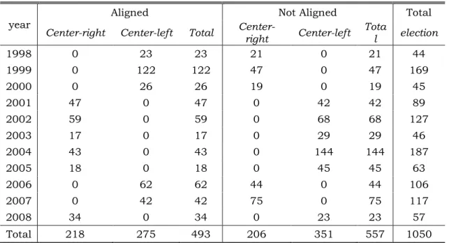
Local elections take place in each municipality every …ve years, but not all at the same time. The large number of municipalities means that local elections occur every year in our sample (See Table 2 for detailed information). On the other hand, national elections have been held in 2001, 2006 and 2008, and at every national election, there has been a change in the ruling government coalition (from left to right in 2001 and from right to left in 2006, and again form left to right in 2008). Figure 1 visualizes the distribution of local governments by winning coalition for each year of the sample period. The …gure is divided into four panels; the …rst and the third correspond to periods when the center-left coalition was in power at the national level, and second and the fourth correspond to the years dominated by a center-right national government.
Insert Table 2 about here Insert Figure 1 about here
In our regression discontinuity design (RDD) setting our treatment is the political alignment with the central government. For this purpose we de …ne the alignment variable, DO, equal to 1 if the mayor’s party-coalition is the same as the coalition in power at the central level. Table 2 presents information on the number of elections by year and by winning coalition for aligned and non-aligned governments. It is interesting to note that the sample is equally split between aligned and non-aligned municipalities.
1 4For example the national law n.42/2009 establishes the need to put in place a mechanism for the aggregation of the necessary parameters to calculatestandard expenditure needs. The aim of the reform, which is currently being implemented, is to replace the old discretionary regime with a formula-based one.
1 5The dataset comprises electoral data from 1998 to 2008 and …scal data and controls from 1998 to 2010. 1 6This is the number of observations for which we observe no missing values for all variables of our dataset.
Next, we construct our assignment variable for the RDD regressions, the margin of alignment,P D, as the di¤erence between the percentage of votes obtained by the winning mayor and the percentage of votes obtained by the runner-up if the winner is aligned with the center, and minus this di¤erence if the mayor is not aligned. So, the sign of the margin of alignment is constructed in a way such that mayors who are (not) aligned with the central government have a positive (negative) margin of victory. If the mayor is elected in the …rst round (because he or she got an absolute majority), the …rst-round results are used, if a second round is held, then second-round results are used instead, (Table AA6 in the Online Appendix reports detailed information on …rst and second round elections). These political indicators have been collected from the Statistical O¢ce of the Italian Ministry of Internal A¤airs.
Table 3 shows the distributions of observations between aligned and non aligned local governments and breaks down the …gures by the margin of alignment. Overall we have 4759 observations, but, if we consider only elections close to treatment thresholds, namely with a value of P D less than either 5% and 2%, the number of observations reduces drastically to 536 and 221 respectively; however the proportion of aligned and non-aligned municipalities remains virtually unchanged. Tables AA7 and AA8 of the Online Appendix report disaggregated information on the number of elections held in each year by winning coalition and alignment status.
Insert Table 3 about here
Our main dependent variables are: (i) current transfers from the central government to municipalities and (ii) local tax revenue. We focus oncurrent expenditures and transfers because they are more likely to track the yearly decisions of central governments at any point in time, unlike investment expenditures, which tend to be set for longer periods of time. All these variables are expressed in real per capita values and data are taken from the Italian Ministry of Internal A¤airs. In particular, current transfers from the central government to municipalities are the item “trasferimenti correnti dallo Stato" in the municipality balance sheet.
Moreover we employ a set of other controls which are generally thought to a¤ect local public …nance outcomes. First, we include variables measuring socio-demographic and geographical characteristics of municipalities, comprising resident population, proportion of population less than 14 and over 65 years old (the source of these variables is the Italian Institute of National Statistics (ISTAT)). Second, we include economic variables, comprising income per capita from real estate and from other sources. The sources for these variables are the Ministry of Finance the Ministry of Interior.
Third, we include other political controls. First, we have dummies recording whether the incumbent mayor (or party) has been re-elected, if the mayor is elected at the second round, and if the municipality is aligned with the regional government. Moreover we also include dummies for political orientation both
at the local and national level (the former equal to one if the mayor is supported by a center-left coalition and that latter equal to one if a center-left government is in power at the national level). Finally, we include an electoral cycle variable that records the number of years since the last local election. The sources for these variables are the Ministry of Interior.
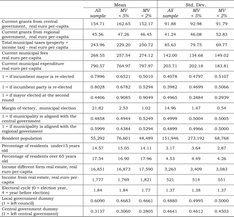
Descriptive statistics for all the variables employed in the regressions are given in Table 4; …gures refer to statistics for the full sample as well as for restricted samples, i.e. for local governments that are close to the treatment threshold, namely within aP Dof …ve and two percentage points.
Insert Table 4 about here
Looking at averageper capitadata for the full sample we can see thatcomuni’s current public expen-ditures amount to 790 Euros per capita, 20% of which is funded by grants from the central government. Figures for the restricted versions of the data set (PD ?5%> P D ?2%) are similar. Looking at our main controls, the values of the standard deviations suggest that there is a lot of variation within each variable included in the data set but not much di¤erence between the three samples.
As a further description of the data, Table AA3 of the Online Appendix presents summary statistics for aligned and non-aligned local governments. We can observe that, municipalities aligned with the central government coalition signi …cantly enjoy more grants from the central government (177.42 and 132.50 Euros per capita), and raise lower taxes (236.88 and 250.85). Finally, note that our samples are almost equally split between aligned and unaligned municipalities, which is the treatment variable we are interested in for the purposes of our analysis.
6
Alignment and Transfers
6.1
Estimation Strategy
In this section we test the prediction of Proposition 1 on the e¤ect of alignment on grant allocation. We use regression discontinuity design (RDD) to address the identi …cation problem in generating unbiased estimates of this alignment e¤ect. The problem is that political alignment is determined by local charac-teristics that are unknown or unobservable by the researcher. To deal with this, we exploit the fact that alignment with the party ruling at the central government changes discontinuously at 50% of the vote share of local parties. This allows us to use sharp regression discontinuity design.
Following this approach, we compare municipalities where the elected mayor is barely aligned with central governments with those where the mayor isbarely unaligned, where “barely aligned” means that the mayor won the election with a tight margin and that the mayor and the central government belong to the same party. Lee (2001, 2008) show that this approach represents quasi-random variation in party
winners, because—as long as there are some unpredictability in voting behavior—when the race is very tight, the identity of the winning party is likely to be determined by pure chance.
There are various ways in which RDD can be implemented using both parametric and non parametric analyses; see Lee and Lemieux (2010) for an excellent survey. The simplest approach is to compare policy outcomes just around the treatment threshold; however this method can produce imprecise estimates and has to rely on a large sample size. Given the relatively limited number of observations available to us around the treatment threshold, our preferred strategy is to use an alternative approach which is based on the use of all available data together with a control function. This approach consists on regressing the dependent variable on a pth-order polynomial in the control function, in addition to the binary treatment indicator.
The model we estimate takes the following form:
lnWl>w=0DOl>w+i(PDl>w;DOl>w) +0[l>w+)w+l+yl>w (15) where Wlw> is the per capita grant to municipalityl at time w>and DOl>w is our alignment dummy that takes value of one if the ruling party at the local level in municipalitylis the same as the party in power at the central level; this is our treatment variable. Finally, P Dl>w, the margin of alignment, already de …ned above, is our assignment variable. Recall that all observations with a positive (negative) PDl>w are municipalities which are aligned (unaligned) with the central government, and observations with a smallP Dl>w in absolute value refer to mayors who won the elections with a very small margin.17
We allow i(PDl>w;DOl>w) to be a swk order polynomial in P Dl>w> with coe¢cients all interacted with DOlw.18 Finally [lw is a vector of control variables, )w is a year dummy, and l is the unobserved heterogeneity. We treat l as a municipality …xed e¤ect. The coe¢cient of interest is 0> which is our alignment e¤ect at the zero threshold, and, following Proposition 1, its expected sign is positive.
As pointed out by Imbens and Lemieux (2008), the above estimation method may be sensitive to outcome values for observations far away from the threshold. To address this issue, as a robustness check, we also implement thelocal linear regressionapproach, which restricts the sample to municipalities in the interval PDl>w2[¡k>+k], wherekis an optimally chosen bandwidth, here selected following the methodology suggested by Imbens and Kalyanaraman (2009).
1 7It is important to emphasize that both the alignment dummy and the assignment variable refer to the previous year ’s observation. This is due to the fact that, in the sample, local and central elections have been held always between April and June, while the allocation of grants is decided by the central government by the end of December and the local …scal policy is decided by local councils usually not later than March.
1 8That is, our control function is: i =
01P Dlw+02P D2lw+===+0sP D s
lw+1DOlwP Dlw+2DOlwP D2lw+===+ sDOlwP Ds=
6.2
The E¤ect of Alignment on Grants
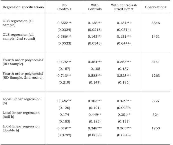
In this section we present the results on the alignment e¤ect on grants. The results are displayed in Table 5. As the dependent variable is the log of the per capita grant, the coe¢cient0in equation (15) has the interpretation of the percentage change in per capita transfer due to the alignment e¤ect.19 In all our speci …cations standard errors are clustered at municipal level.
The table is divided into three panels. In the …rst panel we display results for the so-called OLS regression model (which corresponds to equation (15) in the case of zero-order polynomial in the control function). In the second panel we report the estimated 0 in equation (15) considering the optimal polynomial order in the control function (according to tests reported in Table A1, the optimal polynomial order is the the 4th). The coe¢cients’ point estimates obtained considering all polynomial orders are displayed in Table AA1 of the Online Appendix. We produce two sets of results, the …rst one generated by employing the full RDD sample, and the second one by restricting the sample to those municipalities whose mayor was elected in the second round. By doing so we address a possible concern on the robustness of our results due to the fact that P Dis calculated in the same way (i.e. as the percentage di¤erence in the votes between the winner and the runner up) for elections where the mayor is elected in the …rst round and for those decided in a second round.20
Finally, in the bottom panel we report the results for the local linear regression model, where the sample is restricted to observations within an optimally chosen bandwidth, calculated following Imbens and Kalyanaraman (2009), using the full RDD sample. As a robustness checks we also present results for when the sample is restricted to double as well as half the optimal bandwidth size.
For each speci …cation we propose three variations. In the …rst column, we run the regressions without additional controls, in the second one we include the full set of controls listed in Table 4 as well as year dummies, in the third column we also include a municipality …xed e¤ect. As pointed out by Pettersson-Lindbom (2008), the inclusion of these additional covariates is a way of checking whether alignment status is as good as randomly assigned (conditional oni(PDlw;DOlw))and it should not signi …cantly a¤ect the estimate of the alignment e¤ect. Finally, the last column reports the number of observations.
Insert Table 5 about here
1 9In a previous working paper version of this paper Bracco, Porcelli and Redoano (2013) we present results when the variables are in level, which are qualitatively similar.
2 0Recall that second-round elections are, by de …nition, elections with only two candidates, while in …rst round elections the number of candidates may vary. Second, the fact that a candidate obtains the majority of the votes in the …rst round can itself be interpreted as a sign of high popularity (or, in other words, low political competition in that municipality).This is clearly con …rmed by looking at the summary statistics for the …rst round election dummy reported in Table 4. Taking the full sample, 44% of elections are decided in the second round, but if we look only at close races (i.e. MA less than 5%), the proportion of second round elections goes up to 90%.
A common denominator to all these speci …cations is that the estimated e¤ect of alignment on grants is always positive and generally highly signi …cant. In order to obtain more precise estimates on the magnitude of the alignment e¤ect in Table A1 we report the Akaike Information Criterion (AIC) as well p-values from the goodness-of- …t test (F-test), which provide formal guidance on the choice of the best polynomial order.21 According to these criteria the polynomial order that …ts the data best is the fourth. Using the full sample, this means that ajustaligned municipality should receive between 36% and 47% more grants than ajustunaligned one. The speci …cations with and without controls produce very similar results and it is consistent with the hypothesis that the use of the control function makes redundant the inclusion of further controls. Also the magnitude of these coe¢cients is in line with the results obtained from the local linear regression model using an optimal bandwidth, which, in our case, restricts the sample to the observations within§13%PD. The estimated coe¢cients for the local linear regression model are indeed between 0.33 and 0.44. Moreover it is important to note that RDD coe¢cient estimates are more stable to the introduction of control variables than OLS coe¢cient estimates, showing that the control function reduces the risk of biased estimates due to the problem of omitted variables.
If we consider only municipalities where the mayor was elected in the second round the number of observations drops from 3141 to less than half (1263), but the results remain very similar to the ones previously analyzed. Note also that for this sub-sample, the margin of alignment is on average smaller, as can be clearly seen from Table 4. Full summary statistics for the sample of second round election are displayed in Table AA9 of the Online Appendix.
Finally, in Table A3 of the Appendix, we show that the e¤ect of alignment on grants is stronger at the end of the term, as predicted by the theoretical model. In particular, in Table A3 we estimate the model (15) including, as an additional regressor, the interaction between the alignment dummy and the electoral cycle, de …ned in section 5.2, which records the number of years since the last election in the municipality. The coe¢cient of the interaction term is positive and statistically signi …cant. In the same table we also provide a di¤erent speci …cation of the electoral cycle de …ned by a dummy for the last year of the term. Again, the alignment e¤ect is stronger at the end of the term. These last …ndings are in line with Brollo and Nannicini(2012).
6.3
Graphical Analysis
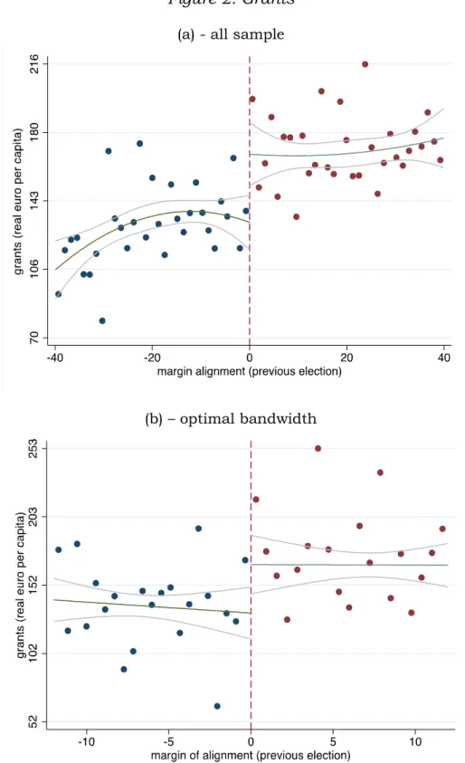
It is also interesting to look at the graphical representation of our RDD results displayed in Figures 2(a) and 2(b). Each …gure shows the margin of alignment, P D>on the horizontal axis, and the per capita grant allocated to each municipality on the vertical axis. Figure 2(a) reports the …tted values from a 2 1Following Lee and Lemieux (2010), this is obtained by jointly testing the signi …cance of a set of bin dummies included as additional regressors in the model. The bin width used to construct the bin dummies is 0.02. A bin width of 0.01 has not been used because was generating to much collinearity in relation to the size of the sample.
running-mean smoothing of per capita grants …tted over the interval [-40, +40] in the PD> performed separately on each side of the cuto¤ point, as well as the 95% con …dence intervals. Following Lee and Lemieux (2010) we include 50 bins in all …gures. Figure 2(b) reports graphical representation of the local linear regression model of per capita grants in theP D …tted over the optimal bandwidth.
Insert Figure 2 about here
The …gures also help with the visualization of the estimated equation (15) to highlight not only the values of 0> the “jump" in the dark line at the zero threshold, but also the shape of the relationship between the outcome variable and the assignment variable. Figure 2(a) not also clearly shows the dis-continuity in the distribution of grants between aligned and unaligned municipalities atP D= 0but also the fact theallaligned municipalities enjoy overall more grant than unaligned ones.
Further analysis in support of the correctness of the procedure we implement is provided in Figure A1 and Table A2. Using the McCrary (2008) procedure, Figure A1 shows a graph of the distribution of P Dcomputed over bins with a bandwidth of 0.01 (100 bins in the graph), along with a smooth 4th-order polynomial model.22 The graph shows no evidence of discontinuity at the cuto¤. Therefore, there is no statistical evidence of manipulation of the assignment variable around the cuto¤. Another important test for the validity of the RD design is to examine whether the covariates do not exhibit any discontinuity in relation to P D. As suggested by Lee and Lemieux (2010) we test the null of discontinuities in all covariates simultaneously estimating a set of regressions where each covariate is a dependent variable, and the explanatory variables are DO> and the polynomial in P D= This system is estimated by Seemingly Unrelated Regression (SUR), and then we perform a chi-square test for joint hypothesis that DO is insigni …cant in all regressions (zero discontinuity). As reported in Table A2 we cannot reject the null hypothesis of zero discontinuity in all covariates in relation to almost all polynomial orders of the margin of victory. Therefore, we can conclude that there is no statistical evidence of discontinuity in the covariates.
7
The Turnover of Incumbents
We now investigate our prediction that the probability of the incumbent mayor being re-elected is higher when aligned with the central government. To this, we estimate the following model:
Ll>h+1=1DOl>h+i(P Dl>h;DOl>h) +0[l>h+h+l+yl>h (16) Note that the temporal unit is now election years, h. The outcome variable is nowLl>h+1>which is equal to one if the winner of the local election at timeh+ 1is the same (or at least belongs to the same party)
as the winner in the previous election (held at timeh) and zero otherwise. As before,i(P Dl>h;DOl>h)is a polynomial function of up to fourth order inPDl>h, where the coe¢cients are interacted withDOl>h=The coe¢cient of interest is1> which is our alignment e¤ect on the probability of incumbent re-election;1 should be interpreted as the di¤erence between the (absolute) probability of re-election of the aligned incumbent and the unaligned one. We expect 1 to be positive.
The variableLl>h+1is calculated in two ways. First, we use a broad de …nition of incumbent,incumbent party, under whichLl>h+1is equal to 1 if the winning mayor at elections held at timeh+ 1in municipality l belongs to the same coalition as the winner of the elections at time h; this is quite consistent with the Italian case where usually the deputy mayor steps in when the incumbent mayor cannot re-run for elections. Second, we consider a narrower de …nition, incumbent candidate, where Ll>h+1 is equal to 1 only if the incumbentmayor is re-elected for the second time at h+ 1and zero otherwise. So under this de …nition we exclude all the cases where the mayor cannot run because of term limits (there is a limit of two consecutive terms for Italian mayors).
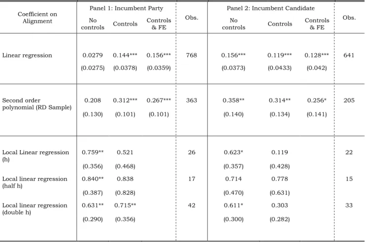
Insert Table 6 about here
Table 6 reports results for di¤erent speci …cations of model (16), using the above two de …nitions of incumbent. Note that the number of observations is now drastically reduced since we are only using elec-tion years; for this reason, we display results only for the regressions where the full sample is employed.23 Note that in all speci …cations standard errors are clustered at municipal level. Using the AIC reported in Table A1 in the Appendix, the polynomial order that …ts the data best is the second for both de …nitions of incumbent, so we will base our discussion on this polynomial order. The complete set of results related to other polynomial orders are reported in Table AA2 of the Online Appendix. Now our RDD sample comprises 363 observations if we use theincumbent partyde …nition forLl>h+1and 205 for theincumbent candidate one. This relatively small number of observations explains why, when we estimate the model using a high polynomial order, the coe¢cients tend to lose signi …cance. The estimated coe¢cients for the incumbent e¤ect are between 0.20 and 0.31 (without and with controls) for the incumbentparty and between 0.25 and 0.35 for the incumbentcandidate, which means that being aligned with the central gov-ernment at the time of election gives local incumbents a strong advantage in comparison to non-aligned ones. The inclusion of …xed and time e¤ects and controls does not a¤ect the magnitude or the signi …cance of the coe¢cients.
2 3Regressions using only second round elections produce very similar results, but given the reduced number of observations (127) standard errors are larger than when the full sample is employed, and this obviously a¤ects the signi …cance of the coe¢cients. Output for 2nd round elections is available upon request.
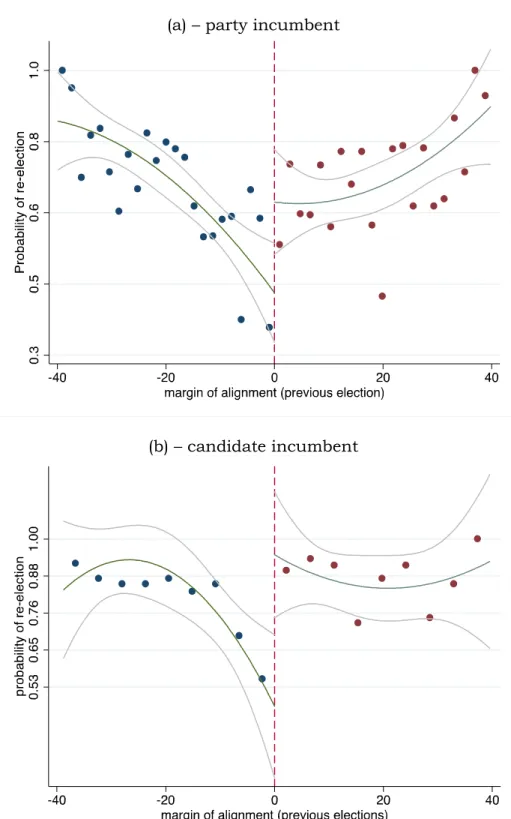
Insert Figure 3 about here
The graphical visualization of our RDD estimations is displayed in Figures 3(a),(b) and it is clearly in line with the regression results. The …gures show the plots of the probability of re-election within each bin againstP D>the margin of alignment in the previous election. Following Lee and Lemieux (2010) we include 50 bins in all …gures. We also report the …tted values from a running-mean smoothing of the variable on the vertical axis performed separately on each side of the cuto¤ point (the darker solid line) as well as the 95% con …dence intervals (the two lighter lines). Both …gures clearly show the “jump" in the probability of incumbent re-election around the zero threshold. Note also that while the probability of re-election for non-aligned mayors is strongly a¤ected by their popularity (i.e. the margin of victory) in the previous elections, this is much less obvious for aligned candidates. At the right hand side of Figure 2(b), the …tted polynomial function is much ‡atter than the one displayed on the left hand side of the …gure. This is consistent with the fact thatmarginal aligned mayors, facing potentially high probability of losing the election, receive extra help, i.e. more grants, from the central government.
8
The Flypaper E¤ect
The …nal step in our empirical analysis is to trace the e¤ect of political alignment on taxes and expendi-tures via the grant. Following Knight (2002), we estimate:
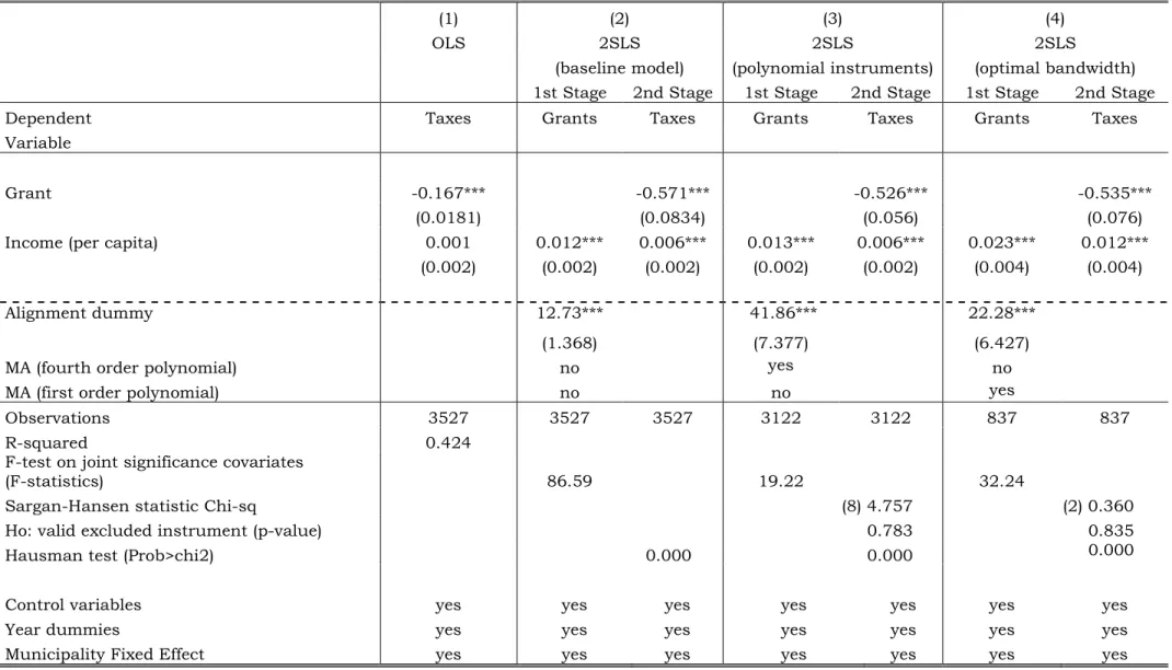
lw=Wlw+0[lw+)w+l+yl>w (17) where lw is a measure of local tax revenue, to proxy for in the theoretical model. Also,[lw includes all the control variables employed in previous regressions and displayed in Table 4. Proposition 3 above suggests that0A A¡1=Of course,Wlwis endogenous, and our previous results suggest that we use the alignment dummyDOlw>as an instrument, which we know to be correlated with Wlw.
Tables 7 reports the main results for model (17). In Table 7, the dependent variable is municipality core tax revenue, which comprises revenue from the (ICI) and the personal income tax, the two main source of municipal tax revenue. As a robustness check we also experiment with alternatives dependent variables (see Tables AA10 and AA11 in the Online Appendix): (i) municipality expenditures net of (national and regional) grants, i.e. revenues from taxes and fees and (ii) municipality expenditures. In all speci …cations, we report standard errors clustered at municipal level, which are robust for serial correlation and heteroscedasticity. We also include time dummies and the full set of controls. Due to space constraints, the coe¢cients on the controls are not reported, with the exception of the per capita private sector income (the variable “income per capita" in the tables), as this is needed for the calculation
of the ‡ypaper e¤ect.24 Finally, municipality …xed e¤ects are included in all speci …cations.
Let us discuss the results displayed in Table 7. The …rst column presents the results when equation (17) is estimated by OLS andWlwis treated as exogenous; in the following columns we present results for the 2SLS whenWlwis instrumented with (i) the alignment dummy only; (ii) the alignment dummy as well as the fourth order polynomial function inP D;(iii) the alignment dummy, and the …rst order polynomial function in PD, and we restrict the sample to those observations falling within the optimal bandwidth employed in the local linear regression on grants above. For the 2SLS speci …cations, we include …rst and second stage regression outputs.
Insert Table 7 about here
When grants are not instrumented (column 1) our results suggest that an increase of 1 Euro per capita in grants reduces local taxes by 0.167 Euros, which means that there is an increase of overall public spending of about 0.83 Euros per capita. By contrast, conditional on the grant, a 1 Euro per capita increase in private income has no e¤ect on public spending. The ‡ypaper e¤ect can be then measured as the di¤erence between one plus the coe¢cient on the grant, and the coe¢cient on private income. So when grants are not instrumented, the ‡ypaper e¤ect in Italian municipalities is calculated to be around 83% percent (1-0.169=0.83).
However the tests reported at the bottom of Table 7 indicate that the grants are endogenous (Hausman test) and that the alignment dummy is a good instrument for it (Sargan-Hansen test), so in the following column of the table we report results for IV estimation. When grants are instrumented (column 2 ) with the alignment dummy, the coe¢cient on grants becomes now -0.571, and it is signi …cant at 1%. Private income per capita becomes signi …cantly positive; however, the size of the e¤ect is very small (a 1 Euro increase in private income gives at most a 1 cent increase in core tax revenue). Overall the extent of the ‡ypaper e¤ect decreases, going down to 0.43% (i.e. 1+(-0.571+0.006)). This means that public spending increases of about 0.43 Euros per capita for each Euro increase in grants. This estimate is almost unchanged when we add a fourth-order polynomial inP Das an additional instrument in column 3. The Sargan-Hansen test displayed at the bottom of the panel suggests that the excluded instruments are valid instruments. Moreover in both cases, an F-statistic on the signi …cance of the …rst stage regressor is very large, suggesting that weak instruments are not a problem (Staiger and Stock (1997)). Finally, in the last column (column 4), we restrict the analysis to those municipalities whose margin of alignment in previous mayoral elections was within the optimal bandwidth (i.e. a value of PD§0=13%). The sample shrinks from 3527 observations to 837. The estimated coe¢cient on the grant is now -0.55. So, overall, 2 4This variable is de …ned as total income declared in the tax return minus real estate income, since real estate income is used as a separate regressor to control for variation in the tax base of the property tax.
the ‡ypaper e¤ect is estimated to be between 43% and 48%. This estimate is in line with other studies in the survey by Inman (2008). In particular, Inman …nds that across a large number of studies, the ‡ypaper e¤ect ranges from about 0.25 to 1.00. It is worth noting that our …nding (namely, that instrumenting decreases the ‡ypaper e¤ect) is similar to what is found in Knight (2002).
In order to test the validity of our results with respect to di¤erent measures oflw>we re-run model (17) using municipality expenditures net of (national and regional) grants (which is equivalent to revenues from taxes and fees) as the dependent variable. Table AA10, included in the Online Appendix, displays the results for this exercise. In Table AA11 we displayed the results for the estimation of model (17) using municipality expenditures as dependent variable. This speci …cation has been usually employed in the past to investigate the extent of the ‡ypaper e¤ect. For both cases the results are consistent with those displayed in Table 7.
9
Conclusions
This paper has explored both theoretically and empirically the e¤ect of political alignment on local public …nance and elections. Our model predicts that aligned jurisdictions are assigned more grants by the central government because a higher grant to aligned mayors (because not directly observed by voters) signals higher competence of that mayor and thus increases the probability of their re-election. Moreover, the model shows that part of the extra grants will be used to reduce taxes, and part to increase local expenditure, implying a ‡ypaper e¤ect.
We test these predictions using a new data set on Italian local public …nance and elections over the 1998-2010 period. Our empirical strategy is based on regression discontinuity design (RDD), exploiting the fact that being or not aligned with the central government changes discontinuously at 50% of the votes at local election. Moreover, the RDD approach also provides a good identi …cation strategy to estimate the relationship between grants and expenditure providing an unbiased measure of the ‡ypaper e¤ect.
Our empirical results are largely consistent with our theoretical predictions. In particular we …nd that, if a municipality is politically aligned with the party in power at the central level, it will be rewarded with an increase in grants between 36% and 47%; moreover, the probability of re-election of aligned municipalities will be between 20% and 35% higher than for non-aligned local governments. Finally, we …nd a positive ‡ypaper e¤ect; 40% of each Euro of extra grants will be used to increase expenditure and 60% will be used, instead, to reduce local taxes.
The theoretical and the empirical analysis showed, in the end, that when local governments are respon-sible for the provision of local public goods, there is a perverse trade-o¤ between the level of discretion in the distribution of intergovernmental grants and the disciplining and selection role of elections. In fact if grants are not formula-based and voters attribute, correctly, most of the credit for providing local public