Optimal Transport and
Elastic Shape Optimization
Dissertation
zur Erlangung des Doktorgrades (Dr. rer. nat.)
der Mathematisch-Naturwissenschaftlichen Fakult¨at
der Rheinischen Friedrich-Wilhelms-Universit¨at Bonn
vorgelegt von
Stefan Simon
aus Andernach
der Rheinischen Friedrich-Wilhelms-Universit¨at Bonn
1. Gutachter: Prof. Dr. Martin Rumpf 2. Gutachter: Prof. Dr. Patrick Dondl Tag der Promotion: 26.11.2019 Erscheinungsjahr: 2019
In this thesis, we consider a novel unbalanced optimal transport model incorporating singular sources, we develop a numerical computation scheme for an optimal transport distance on graphs, we propose a simultaneous elastic shape optimization problem for bone tissue engineering, and we investigate optimal material distributions on thin elastic objects.
The by now classical theory of optimal transport admits a metric between measures of the same total mass. Various generalizations of this so-called Wasserstein distance have been recently studied in the literature. In par-ticular, these have been motivated by imaging applications, where the mass-preserving condition is too restrictive. Based on the Benamou–Brenier formulation we present a novel unbalanced optimal transport model by introduc-ing a source term in the continuity equation, which is incorporated in the path energy by a squaredL2-norm in time of a functional with linear growth in space. As a key advantage of our model, this source term functional allows singular sources in space. We demonstrate the existence of constant speed geodesics in the space of Radon measures. Furthermore, for a numerical computation scheme, we apply a proximal splitting algorithm for a finite element discretization.
On discrete spaces, Maas introduced a Benamou–Brenier formulation, where a kinetic energy is defined via an appropriate (e.g., logarithmic) averaging of mass on nodes and momentum on edges. Concerning a numerical optimization scheme, this, unfortunately, couples all these variables on the graph. We propose a conforming finite element discretization in time and prove convergence of corresponding path energy minimizing curves. To apply a proximal splitting algorithm, we introduce suitable auxiliary variables. Besides similar projections as for the classical optimal transport distance and additional simple operations, this allows us to separate the nonlinearity given by the averaging operator to projections onto three-dimensional convex sets, the associated (e.g., logarithmic) cones.
In elastic shape optimization, we are usually concerned with finding a subdomain maximizing the mechanical stability w.r.t. given forces acting onto a larger domain of interest. Motivated by a biomechanical application in bone tissue engineering, where recently biologically degradable polymers have been explored as bone substitutes, we propose a simultaneous elastic shape optimization problem to guarantee stiffness of the polymer implant and of the complementary set where new bone tissue will grow first. Under the assumption that the microstructure of the scaffold is periodic, we optimize a single microcell. We define a novel cost functional depending on specific entries of the homogenized elasticity tensors of polymer and regrown bone. Additionally, the perimeter is penalized for regularizing the interface of the scaffold. For a numerical optimization scheme, we choose a phase-field model, which allows a diffuse approximation of the elastic objects and the perimeter by the Modica–Mortola functional. We also incorporate further biomechanically relevant constraints like the diffusivity of the regrown bone.
Finally, we investigate shape optimization problems for thin elastic objects. For a numerical discretization, we take into account the discrete Kirchhoff triangle (DKT) element for parametric surfaces and approximate the material distribution by a phase-field. To describe equilibrium deformations for a given force, we study different corresponding state equations. In particular, we consider nonlinear elasticity combining membrane and bending models. Furthermore, a special focus is on pure bending isometries, which can be efficiently approximated by the DKT element. We also analyze a one-dimensional model of nonlinear elastic planar beams, where our numerical simulations confirm and extend a theoretical classification result of the optimal design.
First and foremost, I would like to express my sincere gratitude to my advisor Prof. Dr. Martin Rumpf for his excellent guidance and his constant support throughout my studies and research, sharing his immense knowledge, introducing me into many interesting topics, and putting trust in my mathematical abilities.
I would like to appreciate the willingness of Prof. Dr. Patrick Dondl for co-reviewing my thesis. I would like to thank him and Dr. Patrina Poh for many fruitful discussions on our joint work on bone tissue engineering.
I am grateful to Prof. Dr. Peter Hornung for inviting me to an exciting workshop in Dresden and providing crucial mathematical input on isometric deformations.
I would like to thank Prof. Dr. Carola Sch¨onlieb, Prof. Dr. Jan Maas, Dr. Matthias Erbar, and Dr. Bernhard Schmitzer for interesting collaborations on projects in the field of optimal transport.
I am also indebted to Prof. Dr. Sergio Conti for his excellent training in applied analysis and giving insightful comments and suggestions on my results in elastic shape optimization.
Furthermore, I would like to thank my colleagues at the Institute for Numerical Simulation, University of Bonn, for providing an always pleasant atmosphere, supporting on any hardware and software problems, and various intense conversations, in particular during relaxing and recharging coffee breaks. I would like to offer my special thanks to Dr. Behrend Heeren, Dr. Alexander Effland, Dr. Martin Lenz, Josua Sassen, Marko Rajkovi´c, and Kai Echelmeyer for proofreading parts of my thesis. Besides, I would like to thank Dr. Sascha T¨olkes, Dr. Ricardo Perl, Benedict Geihe, Gabi Sodoge-Stork, and Carole Rossignol.
Last but not least, I want to thank my family for their honest love and everlasting support. In particular, I would like to thank my beloved wife Kirsten Simon for her patience, encouragement, and motivation, as well as her final proofreading of my thesis.
Funding My work has been supported by the German Research Foundation (DFG) through the Bonn Interna-tional Graduate School (BIGS) via the Hausdorff Center for Mathematics (Exzellenzcluster 2047) and the Collab-orative Research Center (SFB 1060).
Abstract iii
Acknowledgements v
1 Introduction 1
1.1 Introduction to Optimal Transport . . . 1
1.2 Introduction to Elastic Shape Optimization . . . 3
2 Mathematical Preliminaries 7 2.1 Radon Measures . . . 7
2.2 Function Spaces . . . 8
2.3 Gamma-Convergence . . . 9
I
Numerical Methods for Optimal Transport
11
3 Foundations in Optimal Transport 13 3.1 The Classical Optimal Transport Problem . . . 133.1.1 Monge’s Formulation . . . 13
3.1.2 Kantorovich’s Relaxation . . . 14
3.1.3 Benamou–Brenier’s Fluid Flow Formulation . . . 15
3.1.4 Wasserstein Gradient Flows . . . 16
3.2 Numerical Methods for the Classical Optimal Transport Problem . . . 16
3.2.1 Overview of Numerical Methods for Optimal Transport . . . 17
3.2.2 Convex Optimization . . . 18
3.2.3 Application of Proximal Splitting Methods to the Flow Formulation . . . 20
4 Optimal Transport with Source Term 23 4.1 A Benamou–Brenier Formula with Source Term . . . 24
4.2 Relation to Previous Work on Optimal Transport with Source Term . . . 25
4.3 Curves of Radon Measures . . . 26
4.4 Existence of Geodesics for a Generalized Optimal Transport Distance . . . 28
4.4.1 Measure-Valued Formulation of the Path Energy Functional . . . 28
4.4.2 Compactness and Existence Result . . . 30
4.5 Finite Element Discretization . . . 34
4.6 Proximal Splitting Algorithm . . . 35
4.6.1 Projection onto the Set of Solutions to the Generalized Continuity Equation . . . 35
4.6.2 Proximal Mappings of Transport and Source Term Cost . . . 36
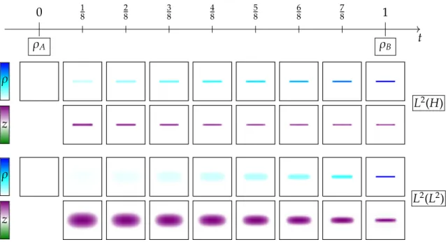
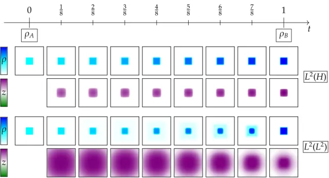
4.7 Numerical Results for Generalized Optimal Transport Geodesics . . . 37
4.7.1 Comparison with the L2(L2)-Model . . . 37
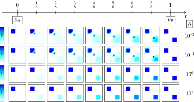
4.7.2 Effect of the Source Term Penalization Parameter . . . 39
4.7.3 Application to Textures . . . 42
4.8 Conclusion and Outlook . . . 43 vii
5.1 A Benamou–Brenier Formula on Graphs . . . 46
5.2 A priori Bounds for Mass and Momentum . . . 49
5.3 Finite Element Discretization . . . 50
5.4 Gamma-Convergence of Finite Element Discretization . . . 51
5.5 Optimization with Proximal Splitting . . . 57
5.5.1 Relaxation via Slack Variables . . . 57
5.5.2 Projection onto Solutions to the Continuity Equation . . . 59
5.5.3 Proximal Mapping of the Edge-Based Kinetic Energy . . . 61
5.5.4 Projection onto the Edge-Based Set . . . 62
5.5.5 Proximal Mappings of Auxiliary Operators . . . 65
5.6 Numerical Results for Optimal Transport Geodesics on Graphs . . . 67
5.6.1 Comparison with the Exact Solution for the Two-Node Graph . . . 67
5.6.2 Exploring the Diffuse Behavior on Simple Graphs . . . 68
5.6.3 Experimental Convergence Rate in Time . . . 72
5.6.4 Experimental Results Related to the Gromov–Hausdorff Convergence in Space . . . 72
5.6.5 Discrete Geodesics on Triangular Meshes of a Human Hand . . . 75
5.7 Simulation of the Gradient Flow of the Entropy . . . 76
5.7.1 Adaption of the Numerical Scheme . . . 76
5.7.2 Numerical Results for Gradient Flows . . . 78
5.8 Conclusion and Outlook . . . 79
II
Numerical Methods for Elastic Shape Optimization
81
6 Foundations in Elasticity and Shape Optimization 83 6.1 Elastic Bodies . . . 836.1.1 Hyperelastic Materials . . . 86
6.1.2 Linear Elasticity . . . 87
6.2 Homogenization . . . 88
6.3 Elastic Shape Optimization . . . 90
6.3.1 Perimeter Regularization and Phase-Field Approximation . . . 91
6.3.2 Computing the Shape Derivative . . . 92
7 Simultaneous Elastic Shape Optimization 93 7.1 Simultaneous Elastic Shape Optimization of a Periodic Microcell . . . 94
7.1.1 State Equations . . . 94
7.1.2 Cost Functional . . . 95
7.2 Hard-Soft Approximation and Perimeter Regularization . . . 96
7.3 Phase-Field Approximation and Finite Element Discretization . . . 97
7.4 Numerical Results for Optimal Periodic Microcells . . . 99
7.4.1 Different Load Scenarios for Equal Material Parameters . . . 100
7.4.2 Influence of the Perimeter Term . . . 101
7.4.3 Influence of Weighting Function . . . 101
7.4.4 Varying Young’s Modulus . . . 101
7.4.5 Realistic Material Parameters for Bone and Polymer . . . 103
7.4.6 The Two-Dimensional Case . . . 103
7.5 Extensions of the Model by Diffusion and Volume Constraints . . . 104
8.1.1 Differential Geometry for Parametric Surfaces . . . 108
8.1.2 Two-Dimensional Models for Elastic Deformations of Thin Shells . . . 111
8.1.3 Overview of Computational Methods for Thin Elastic Shells . . . 113
8.1.4 Discrete Kirchhoff Triangle Element . . . 115
8.2 Shape Design for Mixed Membrane-Bending Models . . . 116
8.2.1 Shape Optimization Problem for a Phase-Field Approximation . . . 116
8.2.2 Finite Element Discretization for Mixed Membrane-Bending Models . . . 117
8.2.3 Numerical Results for Mixed Membrane-Bending Models . . . 119
8.3 Shape Design for Nonlinear Elastic Beams in 2D . . . 125
8.3.1 State Equation for Nonlinear Elastic Beams in 2D . . . 125
8.3.2 Shape Optimization for Nonlinear Elastic Beams in 2D . . . 126
8.3.3 Phase-Field Approximation and Finite Element Discretization . . . 127
8.3.4 Numerical Results for Nonlinear Elastic Beams in 2D . . . 128
8.4 Shape Design for Bending Isometries of Plates . . . 130
8.4.1 Shape Optimization Problem for Bending Isometries . . . 130
8.4.2 Finite Element Discretization for Bending Isometries . . . 131
8.4.3 Numerical Results for Bending Isometries . . . 132
8.5 Conclusion and Outlook . . . 135
Introduction
This thesis contains several contributions, which can be categorized into two mathematical research areas, namely optimal transport and shape optimization of elastic objects. Later, the rigorous mathematical foundations, which are in particular required for these specific projects, are discussed in detail in Chapter 3 and Chapter 6. Further-more, we summarize in Chapter 2 commonly used definitions and well-known theorems, also intending to fix a consistent notation. In the following, we briefly introduce into both fields to give short overviews, including recent developments primarily related to the corresponding topics of this thesis.
1.1
Introduction to Optimal Transport
A Brief History of Optimal Transport. Roughly speaking, the theory of optimal transport is concerned with seeking for the most cost-efficient distribution from a set of sinks to a set of sources. Monge [Mon81] formu-lated such a problem by asking for the transport with minimal cost of a pile of sand into a hole of the same volume. For a general mathematical formulation, sinks and sources are modeled by probability measures. A re-laxed formulation proposed by Kantorovich [Kan42, Kan48] guarantees existence for a certain class of transport cost functions and allows defining the so-called Wasserstein metric on the space of probability measures. Benamou and Brenier [BB00] figured out a dynamical formulation, which can be interpreted as the geodesic equation on the Wasserstein space and thus allows considering it as an infinite-dimensional Riemannian manifold. A groundbreak-ing result linkgroundbreak-ing the geometry of the Wasserstein space with a partial differential equation was established by Jordan, Kinderlehrer, and Otto [JKO98, Ott01], who demonstrated that the heat equation can be understood as the gradient flow of the entropy functional w.r.t. the Wasserstein distance. Further partial differential equations were characterized via gradient flows of suitable energy functionals w.r.t. the Wasserstein distance,e.g., the Keller-Segel equation [BCC08] or the crowd motion model [MRCS10]. For the incompressible Euler equation, considering a relaxation of Arnold’s [Arn66] geodesic formulation in the space of measure-preserving diffeomorphisms, Bre-nier [Bre89] showed that a midpoint of such a geodesic can be found by solving an optimal transport problem. Furthermore, at first glance, unexpected connections of optimal transport to geometrical questions have emerged. On a Riemannian manifold, the displacement convexity of an appropriate entropy functional along Wasserstein geodesics is equivalent to a nonnegative Ricci curvature. Based on this observation, in the independent works of Lott–Villani [LV09] and Sturm [Stu06a, Stu06b], a meaning of a lower Ricci curvature bound on metric measure spaces was given. Besides numerous proofs, the classical isoperimetric inequality was verified by using tech-niques from optimal transport [Kno57], which can be applied to prove generalized versions (see,e.g., Figalli and coworkers [FMP10]). Moreover, the optimal transport problem admits a huge variety of applications in the field of mathematical imaging. For image interpolation, it was considered,e.g., for brains and clouds [HZTA04] and in oceanography [HMP15]. By taking into account an appropriate kernel density estimator, it was used for image segmentation in [PFR12]. In [PPC11], the color transfer of images via optimal transport was studied. A decom-position of an image into cartoon, texture, and noise part was investigated in [BL15]. Many problems arising in economy can also be interpreted in the context of optimal transport,e.g., delivering newspapers or matching be-tween job seekers and jobs [Gal16]. Further applications are related to the classification of texts [KSKW15] or an urban planning model [BS05, BW16].
Numerical Methods for Optimal Transport. Computing optimal transport geodesics in its full generality is a quite challenging task. Therefore it has been solved for numerous special cases. In particular, Wasserstein geodesics between probability measures on the real line can be computed explicitly. For discrete measures, Kan-torovich’s problem becomes a linear program, which can be efficiently solved by the Auction algorithm [BE88]. Benamou and Brenier [BB00] applied duality techniques from convex analysis to compute solutions to their refor-mulated dynamic problem between density functions. For the so-called semi-discrete optimal transport between a density and a discrete measure, methods from algorithmic geometry were investigated in [M´er11, L´ev15]. Further computational methods based on properties of Wasserstein geodesics have been proposed,e.g., in [HZTA04], the polar factorization result by Brenier [Bre91] was used, and in [LR05, BFO10, BFO10], the Monge–Amp`ere equa-tion was solved. In [Sch16a, Sch16b], a sparse multiscale algorithm was developed by incorporating the cyclical monotonicity property. Recently, entropy regularization methods [BCC`15] to compute approximative solutions have turned out to provide an enormous speedup. Overall, most of the equivalent reformulations of the optimal transport problem can be converted into convex optimization problems. Thus, in this thesis, we intensively apply proximal splitting algorithms based on methods from convex analysis.
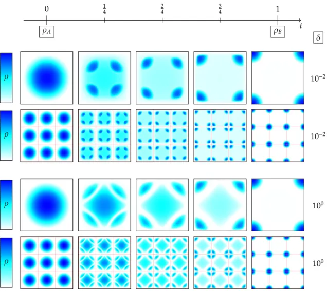
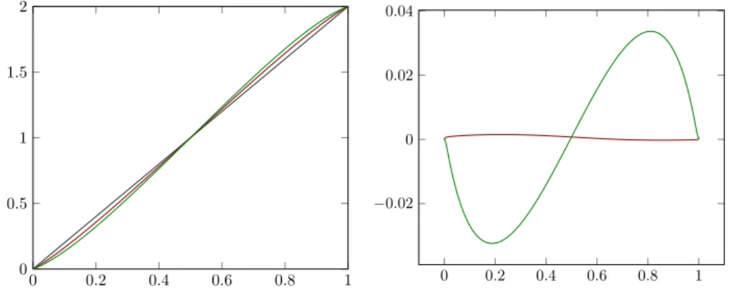
Optimal Transport with Source Term. Naturally, the classical optimal transport distance is defined between two measures of the same total mass, which is for example in the Benamou–Brenier formulation encoded via a continuity equation. This mass preserving property is often too restrictive,e.g., in the context of image warping, where images of different total mass have to be compared. Moreover, an extension of the optimal transport dis-tance to arbitrary positive measures is an interesting question from a theoretical point of view, which has been intensively studied in the literature during the last few years. In general, the resulting problems are often referred to as unbalanced optimal transport. One possibility was studied in [CM10], where the marginal constraints in the Kantorovich formulation were relaxed. For absolutely continuous masses a source term in the continuity equation for the Benamou–Brenier formulation was included in [PR16, PR14]. In [CPSV15] and [LMS15], an interpolating distance between the Wasserstein distance and the Fisher–Rao distance was proposed. Recently, in [CPSV18], an equivalence between such generalized optimal transport models based on the Benamou–Brenier formulation and the Kantorovich formulation was demonstrated for a large class of cost functions. In Chapter 4, we study a novel unbalanced optimal transport model on the space of positive Radon measures. There, we adapt the Benamou– Brenier formulation by a source term in the continuity equation, which is appropriately penalized in addition to the kinetic energy, s.t. we can allow singular sources in space. An example of a transport between measures of different total mass is depicted in Figure 1.1.
1
0.5
0
Figure 1.1: Geodesic between densities of different total mass for an optimal transport model with source term. The mass variable is color-coded in a blue-scale (left).
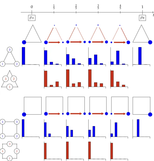
Optimal Transport on Discrete Spaces. The formulations of the optimal transport distance of Monge, Kan-torovich, and Benamou–Brenier can be defined without any additional effort between Borel probability measures on complete and separable metric spaces, so-called Polish spaces, and are equivalent under certain conditions. Fur-thermore, Monge’s problem can be considered on more abstract spaces, as far as there is a notion of measures and distance. On discrete spaces described by an irreducible and reversible Markov transition kernel, Maas [Maa11] proposed a Benamou–Brenier formulation, which also allows understanding the heat equation on a finite Markov chain as the gradient flow of a corresponding entropy functional. The associated discrete optimal transport metric does not coincide with Monge’s formulation. In Chapter 5, we develop a numerical scheme to compute geodesics and gradient flows for this optimal transport distance on finite Markov chains. For appropriate finite element spaces, we prove convergence of minimizing paths for vanishing step size. In Figure 1.2, we depict an example of such an optimal transport geodesic on a discrete space.
Figure 1.2: Geodesic between discrete measures on a triangular mesh of a human hand (left) for an optimal transport model on graphs. The mass variable, which is actually defined on nodal positions, is represented by blue neighborhoods with an area of a proportional size.
Further Related Work. As we have already mentioned, the fluid flow reformulation by Benamou–Brenier can be interpreted as the geodesic equation on the Wasserstein space. Rumpf and Wirth [RW15] introduced a powerful framework for a time discrete geodesic calculus on Banach manifolds, which allows to approximate geodesics and further differential geometric quantities, like the exponential map, parallel transport, and the Riemannian curvature tensor. This approach was,e.g., applied to the space of viscous fluid objects [RW13], the space of images in the context of the metamorphosis model [BER15], and the space of discrete shells [HRWW12]. In [MRSS15], the general framework by Rumpf and Wirth was used to compute optimal transport geodesics for a viscous optimal transport model with density modulation.
1.2
Introduction to Elastic Shape Optimization
An Overview of Elastic Shape Optimization Problems. Optimizing the mechanical stability of an object is a desirable property in numerous engineering applications. In a general framework of mathematical shape optimiza-tion, we ask for the optimal domain within an admissible set, which minimizes a suitable cost functional. Possible applications range from heat diffusion [All02] to fluid dynamics [GHHK15]. Also, the isoperimetric problem can be interpreted as a shape optimization problem, where the area functional has to be minimized over all domains with a fixed volume. In this thesis, we focus on elastic shape optimization problems, where forces are acting on the reference domain of an elastic object and deformations are described via partial differential equations, the so-called state equations. Typical examples of cost functionals studied in the literature are the potential energy [ABFJ97, AJT04], the least square error compared to a target displacement [AJT04], and shape eigenfrequencies [Ped00]. For computational simplicity, in most cases, linear elasticity is taken into account, s.t. the stored elastic, the potential and the free energy coincide for the equilibrium displacement. These three functionals were com-pared in [PRW12] for nonlinear elasticity, where in particular global minimizers of the free energy do not have to be unique. A worst-case scenario is given by choosing the most expensive of these equilibrium deformations. Usu-ally, the volume of the elastic object is additionally penalized in the cost functional, or a constraint on the maximal amount of volume is integrated into the optimization problem. Nevertheless, such shape optimization problems are in general ill-posed because a minimizing sequence of characteristic functions does not necessarily converge to a characteristic function, and thus the limiting object cannot be characterized as a set. A possible relaxation is based on the theory of homogenization [ABFJ97], where a composite structure determined by its local volume fraction and the effective elasticity tensor is taken into account. Alternatively, in [PRW12], the perimeter of the domain was added to the cost functional. Such a regularization was originally proposed in [AB93] for a scalar-valued prob-lem. A worst-case scenario concerning the uncertainty of a single force acting on the elastic object was studied in [AD14]. For a scenario where multiple loads are acting on the elastic object, several stochastic interpretations to define an associated average cost functional are considered. In the context of a two-stage stochastic program-ming formulation, in [CHP`08], the expected value was used as compliance functional. Nonlinear risk measures like the expected excess, or the excess probability were investigated in [CHP`11]. In [CRST18], the concept of stochastic dominance was transferred to elastic shape optimization by asking for an object with minimal volume s.t. compared to a given benchmark shape the stochastic dominance constraints given by nonlinear risk measures are satisfied.
Numerical Methods for Elastic Shape Optimization. For a numerical solution scheme to compute an optimal shape, we have to choose a finite-dimensional representation of the elastic object and a corresponding optimization algorithm. A discretization of the elastic object with a finite mesh was,e.g., implemented in [SSW15]. Unfortu-nately, this requires a remeshing in each optimization step, which is algorithmically quite demanding, especially if the topology of the mesh should change during the optimization process. Level-set functions [CHP`08, CHP`11] to represent the domain by the zero-level set, or phase-field functions [PRW12], which are in particular advan-tageous to approximate the perimeter functional, have turned out to be more practicable. If the optimal shape is expected to be of a special structure, determining an appropriate set of parameters could simplify the optimization. For example, in [JKZ98], a simple truss model was investigated. For the optimization algorithm, a naive solution scheme is the so-called evolutionary structural optimization (ESO) method [XS93], where, starting on a fixed fi-nite element mesh, those elements with the least contribution to the stiffness are successively removed. Besides, the bi-directional ESO (BESO) [HX10] also allows inserting elements, which might be useful for a fixed volume constraint. However, there is no guarantee that these schemes provide an optimal shape, and, in particular, the so-lution is mesh-dependent. The homogenization method [ABFJ97] makes use of an explicit formula for an optimal microstructure in linear elasticity, which is given by sequential laminates. Algorithmically, homogenization was used to alternatingly optimize the microstructure and the density on the macroscale. Instead of using the optimal laminate microstructure, the solid isotropic material with penalization (SIMP) method [Ben89] interpolates the material value on each element depending on the density function. In this thesis, we make use of first-order meth-ods, which require to compute the first derivative of the cost functional w.r.t. the elastic object, the so-called shape derivative. This approach was,e.g., applied in [PRW12] for a phase-field model, which we also take into account to discretize the corresponding elastic objects appearing in the specific applications. For a volume constraint, in [AJT04], a Lagrange multiplier was used. A Cahn–Hillard gradient flow with a volume constraint was considered in [ZW07] for a multiphase model. Additional inequality constraints were treated by interior-point methods,e.g., the thickness of trusses in [JKZ98].
Simultaneous Elastic Shape Optimization. The shape optimization problems described above aim to find an optimal subdomain representing the elastic object within a larger domain of interest, which then automatically defines a domain splitting, where the complementary set is considered as void material. In [THD02, TD04], a si-multaneous shape optimization problem was investigated by considering the heat conductivity on a subset and the electrical conductivity on the complementary set. More precisely, the optimal domain splitting was sought, s.t. the sum of the traces of the associated homogenized tensors is optimized. For this scalar case, it was conjectured that optimizers are given by domains bounded by periodic minimal surfaces,e.g., the Schwarz P surface. However, in [Sil07] an upper bound for the sum of the traces of the homogenized tensors was derived, which was numerically compared with the corresponding value for a Schwarz P surface and a significant difference to this upper bound was experimentally obtained. In Chapter 7, we propose a similar simultaneous shape optimization problem by taking into account a novel cost functional depending on specific entries of the homogenized elasticity tensors of both subdomains. This formulation is motivated by an application in bone tissue engineering, where biologically degradable polymer implants with a certain microstructure are used as bone substitutes. Incorporating the stiffness of both subdomains in the optimization process guarantees mechanical stability of the polymer implant as well as the regeneration of bone on the complementary set. Furthermore, we adapt the model by additional biologi-cally relevant constraints. In particular, we enforce diffusion constraints on the regrown bone. We show possible optimized periodic microstructures in Figure 1.3.
Figure 1.3: Optimized periodic microstructures for bone tissue engineering (here for different material parameters of regrown bone).
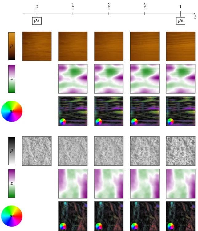
Shape Design of Thin Elastic Objects. Thin elastic objects are a special class of curved elastic bodies, which are significantly smaller in one direction. Such thin structures frequently appear in aerodynamics [HZ14, KPRA18, SS13], where in particular airfoils are optimized w.r.t. the aerodynamic drag. Further applications can be found in electrostatics [BCO`15] and automotive engineering [Ble14]. From a theoretical point of view, the behavior of these thin elastic objects has been well-understood viaΓ-convergence results for vanishing thickness. Different
scalings lead to a membrane theory [LDR95, LDR96] describing tangential distortion on the surface and a bending theory [FJM02, FJMM03] taking into account isometric deformations. In numerical simulations, the corresponding elastic energies have often been combined. Numerous discretization methods have been proposed to approximate thin elastic objects and their deformations, where the essential difficulty is due to curvature terms in the bending energy functional involving second derivatives of the deformation. On quadrilateral meshes, nonuniform rational B-splines (NURBS) [HCB05] allow arbitrary regularity. A fully conforming discretization on triangular meshes is given by loop subdivision finite elements [COS00]. In practice, methods from discrete differential geometry have turned out to be extremely efficient [GHDS03]. To simulate pure bending isometries on plates, in [Bar13] a numerical approximation scheme was provided by making use of the discrete Kirchhoff triangle (DKT) element [BBH80]. The optimal design of shells via composite material lamination was considered in [SL05]. The finite mesh itself was optimized in [BC18] by taking into account loop subdivision surfaces and linear elasticity as in [COS00]. In [VHWP12], NURBS were investigated to construct self-supporting surfaces. In Chapter 8, we study shape optimization problems for thin elastic objects. To describe a material distribution, we use a phase-field discretization. Then we investigate different elastic energies, in particular, nonlinear elasticity and an isometry constraint. In Figure 1.4, we depict optimal designs.
Figure 1.4: Optimal material distributions on a thin plate under certain volume conditions (here for different volume constraints). The hard material is colored in orange.
Mathematical Preliminaries
The following chapter is mainly considered to fix overall terminology and notation. In this thesis, we investigate many different objects,e.g., images, graphs, rods, plates, shells, and solids. For mathematical modeling of these objects, we take into account different function spaces, possibly also including a time component. Especially, we make use of the space of Radon measures, which we introduce in Section 2.1. Further relevant function spaces are defined in Section 2.2. Finally, we consider the concept ofΓ-convergence in Section 2.3, which plays an important
role throughout this thesis. For a more detailed introduction, we refer the reader to the books [FL07], [EG15], [AFP00], [Alt16] for functional analysis and [Bra06], [DM93] forΓ-convergence.
2.1
Radon Measures
In the following, we define the space of Radon measures and summarize some essential properties. We start to recall basics from measure theory. In particular, we define measures on a generic setXwith aσ-algebraEĂPpXq. Definition 2.1.1(Measures and Total Variation). LetXbe a nonempty set.
1. On a measure spacepX,Eqa mapµ:EÑ r0,8sis a positive measure ifµpHq “0andµisσ-additive on
E. If the same holds for a mapν:EÑR, we call it a signed measure. Moreover,ν:EÑRmwithmPN` is a vectorial measure if each component is a signed measure.
2. Letν:EÑRbe a signed measure. Then the total variation|ν|TVforEPEis given by
|ν|TVpEq:“sup # ÿ nPN |νpEnq| : E“ ď nPN
EnforEnPEpairwise disjoint +
and defines a positive and finite measure (see [AFP00, Theorem 1.6]). For a vectorial measureν:EÑRm we define the total variation by|ν|TVpEq:“řim“1|νi|TVpEq.
We remark that there are different terminologies used in the literature, where a measure might denote either a positive or a signed measure. Furthermore, some approaches are based on so-called outer measures, which are defined on arbitrary subsets (e.g., in [EG15]).
Now, to define Radon measures, some topological information on the setXis required. Then, we denote by BpXqthe Borelσ-algebra, which is defined as the smallestσ-algebra onXcontaining all open sets. Due to our applications, we restrict to the case thatX“DĂRdis a subset ofRd.
Definition 2.1.2(Radon Measures). Consider the measure spacepD,BpDqqforDPBpRdq.
1. A positive measureµ:BpDq Ñ r0,8sis a positive Radon measure ifµpKq ă 8for allKĂDcompact. A signed measureν:BpDq Ñ Ris a signed Radon measure if|ν|TV is a positive Radon measure and a vectorial measureν:BpDq Ñ Rm is a vectorial Radon measure if each component is a signed Radon measure.
2. We denote by
(a) M`pDqthe set of all positive Radon measures,
(b) MpDqthe set of all signed Radon measures, and (c) MpD,Rmqthe set of all vectorial Radon measures.
In the following, we further restrict to a compact set D Ă Rd. Then a positive Radon measure is just a finite Borel measure and thus a signed measure. An important characterization of Radon measures is given by the following duality result, which allows us to identify the space of signed Radon measuresMpDqas the topological dual of the space of continuous functionsCpDqendowed with the norm}f}CpDq:“supxPD|fpxq|.
Theorem 2.1.3(Duality of Radon Measures). LetDĂRdbe a compact set. Then every bounded linear functional L:CpDq ÑRis represented by a unique signed Radon measureνPMpDqin the sense that
Lpfq “ ż
D
f dν @f PCpDq. (2.1)
Conversely, every functionalLof type(2.1)forνPMpDqis a bounded linear functional onCpDq.
Proof. See [FL07, Theorem 1.196].
Hence, a sequence of Radon measurespνnqnPNĂMpDqconverges weakly-˚toνPMpDqif
ż D f dνnÑ ż D f dν @f PCpDq.
Furthermore, sinceCpDqis a separable space, every bounded sequencepνnqnPNĂMpDqof signed Radon
mea-sures has a weakly-˚converging subsequence (see [Alt16, Theorem 8.5]).
2.2
Function Spaces
Here, we summarize several properties of Sobolev functions and functions of bounded variation.
In the following, letDĂRdbe a domain. First, fork-times continuously differentiable functions f,gPCkpDq withkPN`, we defineDkf¨Dkg:“ř i1,...,ik“1,...,kB k i1,...,ikfB k i1,...,ikgand|D kf|:“`Dkf¨Dkf˘12.
Lebesgue and Sobolev Functions For a measurable function f:DÑRd, we recall the norms
}f}LppDq:“ ˆż D| fpxq|pdx ˙1 p forpP r1,8q, }f}L8pDq:“esssup xPD |fpxq| “inftCě0 : |fpxq| ďCfora.e.xPDu, }f}Wm,ppDq:“ ˜m ÿ k“0 }Dkf}pLppDq ¸1 p formPN, pP r1,8q, }f}Wm,8pDq:“ max k“0,...,m}D kf} L8pDq formPN,
where the derivatives appearing in the definitions of the Sobolev norms} ¨ }Wm,ppDq for p P r1,8s have to be
understood in the distributional sense.
We say thatD Ă Rd has Lipschitz boundary, if for all x P BDthere exists a neighborhood Uof x and a Lipschitz functionL:Rd´1ÑRs.t.DXU“ ty“ py1, . . . ,ydq PU : yd ąLpy1, . . . ,yd´1qu. Then, we define the spaceW0m,ppDqas the closure ofC8
c pDqw.r.t. theWm,ppDq-norm. Later, we make use of the following two theorems.
Theorem 2.2.1(Korn’s Inequality). LetDĂRdbe a domain with Lipschitz boundary. Then there is a constant cą0s.t. }Du}2L2pDqďc ´ }u}2L2pDq` }εpuq}2L2pDq ¯ (2.2)
for alluPW1,2pD,Rnq. Here,εpuq:“ Du`DuT
2 denotes the symmetrized gradient.
Proof. See [Nit81].
Theorem 2.2.2(Sobolev Embedding). LetDĂRdbe a domain with Lipschitz boundary. 1. Letm1 ąm2PNandp1,p2P r1,8qwithm1´pd1 ąm2´pd2.
Then the embeddingid :Wm1,p1pDq ÑWm2,p2pDqis continuous and compact. 2. LetmPN`,kPN,pP r1,8q, andαP r0,1ss.t.m´d
p ąk`α. Then the embeddingid :Wm,ppDq ÑCk,αpDqis continuous and compact.
Proof. See [Alt16, Theorem 10.9 and Theorem 10.13].
Functions of Bounded Variation Next, we introduce the space of functions of bounded variation. Definition 2.2.3(Functions of Bounded Variation). LetDĂRdbe a domain.
1. The space of functions of bounded variation is defined by
BVpDq:“ tuPL1pDq : DuPMpD,Rdqfor the distributional gradientu. 2. ForuPBVpDqthe norm is given by}u}BVpDq:“ }u}L1pDq` |Du|TVpDq.
3. For a sequenceukPBVpDqanduPBVpDqwe say thatukconverges weak-˚touinBVifukÑustrongly inL1pDqandDu
ká˚ DuinMpD,Rdq. Then the following embedding theorem holds.
Theorem 2.2.4(Embedding in BV). LetD Ă Rdbe a domain with Lipschitz boundary and let1 ď p ă d d´1.
Then the embeddingid :BVpDq ÑLppDqis continuous and compact.
Proof. See [AFP00, Theorem 3.47].
2.3
Γ
-Convergence
Many problems appearing in this thesis result in minimizing an energy functionalE:X Ñ RY t8uon some metric spaceX. Typically, to approximate a minimizer ofE, we take into account a finite spaceXh ĂXand a suitable functionalEh:Xh ÑRY t8u, s.t. we can numerically compute a minimizer ofEh. Further functionals considered in this thesis similarly arise as limits of functionalsEh : Xh Ñ RY t8uforh Ñ 0. However, the convergence ofEh Ñ Ein a common topology of the functionals is a too strong requirement, but we are only interested in the convergence of the minimizers ofEhto the minimizer ofE. This can be established by using the concept ofΓ-convergence.
Definition 2.3.1(Γ-Convergence). LetpX,dqbe a metric space andEk:XÑRY t8uforkPN. We say that the sequence of functionalspEkqkPNΓ-converges to a functionalE:XÑRY t8uif
1. theΓ-liminf condition holds,i.e., for allpxkqkPNĂXwithxkÑxPXwe have Epxq ďlim inf
2. and theΓ-limsup condition holds,i.e., for allxPXthere exists a sequencepxkqkPNĂXwithxkÑxs.t.
Epxq ělim sup kÑ8
Ekpxkq. (2.4)
Note that (2.3) implies that we actually have equality in (2.4). The sequence satisfyingEpxq “limkÑ8Ekpxkq is called a recovery sequence.
Definition 2.3.2(Equicoercivity). LetpX,dqbe a metric space andEk:XÑRY t8uforkPN. The sequence of functionalspEkqkPNis equicoercive if for allrPRthere is a compact setKrĂXs.t.txPX : Ekpxq ďr@kP
Nu ĂKr.
Thus, for a sequencepxkqkPNwith uniformly bounded energyEkpxkq ďr, the equicoercivity condition implies
convergence of a subsequencexkl ÑxPX. Together with theΓ-convergence, this guarantees that minimizers of Ekconverge to a minimizer ofE.
Theorem 2.3.3(Fundamental Theorem ofΓ-Convergence). LetpX,dqbe a metric space andEk:XÑRY t8u forkPN. We assume that the sequencepEkqkPNis equicoercive andΓ-converges toE:XÑRY t8u. Then
min
xPXEpxq “klimÑ8xinfPXEkpxq.
Proof. See [Bra06, Theorem 2.10].
Consequently, if a sequencexk Ñx˚ is asymptotically minimizing,i.e., it satisfiesEkpxkq “infxPXEkpxq ` op1q, thenx˚is a minimizer ofE.
Later, we make use of the following lower semi-continuity result, which allows proving theΓ-liminf
inequal-ity (2.3) for a large class of functionals.
Theorem 2.3.4(Ioffe). Let D Ă Rd be open and bounded. Furthermore, let f:DˆRp`q Ñ r0,8s be a measurable function, s.t.ps,zq ÞÑ fpx,s,zqis lower semi-continuous for a.e.x PDandzÞÑ fpx,s,zqis convex for anyxPDand anysPRp. Then, for sequencesu
hÑustrongly inL1pD,RpqandvhÑvweakly inL1pD,Rqq, we have ż D fpx,u,vqdxďlim inf hÑ0 ż D fpx,uh,vhqdx.
Numerical Methods for Optimal Transport
Foundations in Optimal Transport
The first part of this thesis is concerned with two different types of optimal transport distances, where we primarily focus on numerical methods to compute corresponding geodesic interpolation paths. In this chapter, we first give an introduction to the basic theory of optimal transport and related mathematical foundations. In particular, in Section 3.1, we define theL2-Wasserstein distance on the space of Borel probability measures. To compute solutions for this classical optimal transport distance, various algorithms have been developed, which we partially summarize in Section 3.2. Furthermore, since in Chapter 4 and Chapter 5 we intensively make use of so-called proximal splitting methods, we collect the related concepts from convex analysis.
3.1
The Classical Optimal Transport Problem
In the following, we introduce three different formulations of the optimal transport problem, namely those of Monge, Kantorovich, and Benamou–Brenier. For transport costs given by the Euclidean distance, this leads us to the corresponding Wasserstein metric on the space of Borel probability measures. Moreover, we briefly discuss gradient flows on the Wasserstein space and the fundamental connection to the heat equation. For a more general overview of the theory of optimal transport, we refer the reader to the well-established books [AGS08, San15, Vil03, Vil09].
3.1.1
Monge’s Formulation
A first version of the optimal transport problem was already formulated in 1781 by Monge [Mon81], who asked for the minimal cost to transport a pile of sand into a hole of the same volume. For a mathematical model, source and sink are described by Borel probability measuresµAPPpXqandµB PPpYq, where we restrict to the case that X,YĂRdare compact sets. To define a transport of the mass represented by the measureµ
A, we take into account a transport mapT:XÑY. Then, to guarantee that the mass is transported byTto a distribution corresponding to the measureµB, a matching condition is required.
Definition 3.1.1(Pushforward). LetµPPpXqandT:XÑYBorel measurable. We define the pushforwardT#µ ofµthroughTas
T#µpEq:“µpT´1pEqq for allEPBpYq. (3.1) We say that a transport mapTmatchesµAtoµBifT#µA“µB. Moreover, a transport cost functionc:XˆYÑ r0,8sdescribes the cost to move a particle from a positionx PXto a positionyPY. Then Monge’s problem in its general formulation is to find a transport mapThaving minimal transport cost, which is given by
inf "ż Xcpx ,TpxqqdµApxq : T:XÑYBorel measurable,T#µA“µB * . (3.2)
We focus on the case thatX“Y“Dfor a compact and convex domainDĂRd. Note that the set of all Borel probability measures onDis defined as a subset of positive Radon measures
PpDq “ tµPM`pDq : µpDq “1u. 13
By duality of Radon measures (see Theorem 2.1.3), the matching condition (3.1) is equivalent to ż D fpTpxqqdµApxq “ ż D fpxqdµBpxq @f PCpDq.
Furthermore, we restrict the transport cost function to the Euclidean distancecpx,yq “ |x´y|2. Because of the convexity assumption on the domainD, the distance onDis induced from the distance onRd.
Remark3.1.2. For nonconvex domains, we could take into account the path length fromxtoy. More generally, we could define Monge’s problem for underlying smooth manifolds or even on separable complete metric spaces, so-called Polish spaces, by using the squared distance as transport cost. For noncompact domains, we have to restrict the space of Borel probability measures to guarantee that the integralşXcpx,TpxqqdµApxqis finite. A sufficient condition in the case of the cost functioncpx,yq “ |x´y|2is to require bounds on the second moment,
i.e.,µA, µBPP2pXq:“ tµPPpXq : şX|x|2dµpxq ă 8u.
Unfortunately, Monge’s problem (3.2), in general, does not admit existence nor uniqueness. Example 3.1.3(Nonexistence and Nonuniqueness for Monge’s Problem).
1. LetD“ r´1,1s,µA“δ0andµB “ 21pδ´1`δ1q, whereδpdenotes the Dirac measure at the pointpPD. Then there does not exist a transport mapTbetweenµAandµB, since otherwise
fpTp0qq “ ż D fpxqdT#µApxq “ ż D fpxqdµBpxq “ 1 2pfp´1q `fp1qq for all f PCpDq. In other words, we cannot split a single point.
2. LetD“ r0,1s2,µ
A“ 12pδp0,0q`δp1,1qqandµB “ 12pδp1,0q`δp0,1qq. Then an optimal transport map could
mapp0,0qtop0,1qandp1,1qtop1,0q, but also the opposite way is optimal.
3.1.2
Kantorovich’s Relaxation
To cope with the existence problem, Kantorovich [Kan42, Kan48] proposed a relaxation of Monge’s formulation by embedding the transport mapT:DÑDbetweenµAandµB into the product spaceDˆDby considering a so-called transport planπ“ pidˆTq#µA. SinceTfulfills the pushforward matching condition (3.1), the transport planπsatisfies the marginal constraints
pproj1q#π“µA and pproj2q#π“µB,
whereprojifor i “ 1,2denotes the projection on thei-th component. More generally, we define the set of all Borel probability measures on the product space with marginal constraints by
ΠpµA, µBq “ πPPpDˆDq : pproj
1q#π“µA, pproj2q#π“µB (
.
Then Kantorovich’s problem is given by inf "ż DˆDcpx ,yqdπpx,yq : πPΠpµA, µBq * (3.3) and the following existence result holds.
Theorem 3.1.4 (Existence of Solutions). Suppose thatc: DˆD Ñ RY t8uis lower semi-continuous and bounded from below. Then Kantorovich’s problem(3.3)admits a solution.
Proof. See [San15, Theorem 1.5].
Under the condition that the initial measureµA is absolutely continuous w.r.t. the Lebesgue measure onD, uniqueness of the optimal transport plan can be established by applying Brenier’s polar factorization result [Bre91], which allows decomposing a density function into a gradient of a convex function up to a concatenation with a measure-preserving map. In this case, the solution to Monge’s and Kantorovich’s problem coincide.
Theorem 3.1.5(Brenier’s Polar Factorization). We consider the specific transport cost functioncpx,yq “ |x´y|2.
LetµA, µBPpDqwithµA “ρALDfor a density functionρA. Then there exists a unique optimal transport map Tsolving Monge’s problem, andT “∇ψis theµA-a.e. unique gradient of a convex functionψ. Moreover, the unique optimal transport plan solving Kantorovich’s problem is given byπ“ pidˆ∇ψq#µA.
Proof. See [San15, Theorem 1.22].
In the casecpx,yq “ |x´y|2, the relaxed problem (3.3) defines a metric on the space of Borel probability measures, the so-calledL2-Wasserstein distance.
Definition 3.1.6(Wasserstein Distance). LetµA, µB P PpDqbe two Borel probability measures. We define the L2-Wasserstein distanceWbetweenµ
AandµBby WpµA, µBq:“inf "ż DˆD| x´y|2dπpx,yq : πPΠpµA, µBq *1 2 . (3.4)
We refer the reader to [San15, Proposition 5.10] for a proof thatWis indeed a metric onPpDq. Moreover,
Wmetrizes weak-˚-convergence onPpDq(see [San15, Theorem 5.10]). Regarding a numerical optimization scheme to compute an optimal transport plan solving Kantorovich’s problem (3.3), it is useful to consider the corresponding dual formulation
sup "ż D fpxqdµApxq ` ż D gpyqdµBpyq : pf,gq PCpDq ˆCpDq, fpxq `gpyq ďcpx,yq * .
3.1.3
Benamou–Brenier’s Fluid Flow Formulation
In [BB00], Benamou and Brenier transferred Monge’s problem into a continuum mechanics framework and derived an equivalent representation of the Wasserstein distance (3.4) heuristically. This dynamical formulation takes into account a curve of probability measures µ:r0,1s Ñ PpDq connectingµp0q “ µA withµp1q “ µB and a corresponding Eulerian velocity fieldv: r0,1s ˆD Ñ Rd. Here, we assume that µ is a curve of probability densitiesρ,i.e.,µptq “ρptqL for alltP r0,1s. Then we can formally define the kinetic energy
Etranspρ,vq “ ż1 0 ż D ρpt,xq|vpt,xq|2dxdt.
Furthermore, a mass-preserving condition is given by the continuity equationBtρ`divpρvq “0,i.e., solutions to this equation satisfyşDρpt,xqdx“şDρp0,xqdxfor alltP r0,1s. We denote byCEpρA, ρBqthe set of all weak solutionspρ,vqof the continuity equation with initial conditionρp0q “ρAand final conditionρp1q “ρB. It turns out that Monge’s formulation (3.2) of the optimal transport problem can be rewritten by minimizing the kinetic energy over all corresponding curves of mass and velocity, which solve the continuity equation,i.e.,
WpρAL, ρBLq “inftEtranspρ,vq : pρ,vq PCEpρA, ρBqu 1
2 . (3.5)
To rigorously formulate (3.5) on appropriate function spaces, the curveµis required to be absolutely continuous in time. Moreover, the continuity equation has to be defined in a weak sense. Then, one possibility (see,e.g., [AGS08, Chapter 8]) is to define the velocity at timetin a the function space depending on the measureµptqat the specific time. Later, we apply a different approach by making use of a change of variables. Instead of the pair mass and velocitypρ,vq, we consider the pair mass and momentumpρ,m“ρvq. Then it can be shown that the distance defined by the Benamou–Brenier formulation coincides with the Wasserstein distance (see [San15, Theorem 5.28]). Furthermore, for an absolutely continuous initial measureµA“ρALDand an optimal transport planπ“ pidˆ∇ψq#µAas in Theorem 3.1.5, the linear interpolation of the identity and the optimal transport map ∇ψunder the pushforward w.r.t.µA
µptq “ pp1´tqid`t∇ψq#µA“ pid`tvq#µA
is the solution to Benamou–Brenier’s problem and satisfies the property of a constant speed geodesic
Wpµpsq, µptqq “ |t´s|WpµA, µBq @s,tP r0,1s.
For now, we consider the definition ofWin (3.5) just formally and refer to Chapter 4 for a rigorous formulation of a generalized optimal transport distance.
3.1.4
Wasserstein Gradient Flows
In [JKO98], a fundamental connection between gradient flows w.r.t. the Wasserstein metric onRd and the heat equation was established. First, we recall that for a functionFPC1,1pRd,Rq, the solution to the Cauchy problem
#
x1ptq “ ´∇Fpxptqq fortą0,
xp0q “x0 can be approximated by an implicit Euler scheme
xτ0 “x0, xτ k`1Parg min xPRd Fpxq `|x´x τ k|2 2τ forkPN, (3.6)
whereτą0is a fixed step size. Now, we define the entropy functionalH:L1pRd,r0,8sq ÑRY t8uby Hpρq “
ż
Rdρp
xqlogpρpxqqdx.
More generally, for a smooth potentialV, we consider the functionalFpρq “Hpρq`şRdVpxqρpxqdx. Motivated
by the finite-dimensional and smooth case in (3.6), the so-called minimizing movement scheme is defined by the iteration ρτ0 “ρ0, ρτk`1P arg min µPP2pRdq:µ“ρL Fpρq ` 1 2τWpρ, ρ τ kq 2 forkPN. (3.7)
It was shown in [JKO98, Proposition 4.1] that for an absolutely continuous initial condition, there is a unique dis-crete solution trajectorypρτ
kqkPN. Furthermore, in the limitτÑ0, the following interpretation as the Wasserstein gradient flow ofF was given.
Theorem 3.1.7(Gradient Flow of Entropy). Givenµ0 PPpRdqwithµ0“ρ0LdandFpρ0q ă 8. LetpρτkqkPN
be the discrete solution trajectory obtained by(3.7)and defineρτpt,xq “ρτ
kpxqfortP rkτ,pk`1qτq. Thenρ
τ áρ
inL1pR
`ˆRdqforτ Ñ 0, whereρ P C8pp0,8q ˆRdqis the unique solution to the Fokker-Planck equation
Btρ´∆ρ´divpρ∇Vq “0withρptq Ñρ0inL1fortÑ0.
Proof. See [JKO98, Theorem 5.1].
Note that in the special caseV“0we recover the heat equationBtρ´∆ρ“0. For a more detailed introduction to Wasserstein gradient flows, we refer the reader to [San15, Chapter 8], where, in particular, further examples of partial differential equations and corresponding energy functionals are summarized.
3.2
Numerical Methods for the Classical Optimal Transport Problem
Numerous applications have led to plenty of computational methods to solve the optimal transport problem at least for some special cases. Here, we first give a brief overview of numerical algorithms and collect the basic ideas corresponding to the different formulations of the optimal transport distance. Later, we study optimal transport distances based on the Benamou–Brenier formulation (3.5), which has already been used in [BB00] for the numer-ical purpose by applying a suitable change of variables. Then, the optimal transport problem turns into a convex optimization problem, which is solved via an augmented Lagrangian and duality techniques from convex analysis. In [PPO14], it was shown that a proximal splitting algorithm leads in fact to the same optimization scheme, which requires to solve a linear system corresponding to an elliptic problem on the time-space domain and pointwise projections onto a convex set. Here, we introduce the basic concepts from convex analysis, which are necessary for a proximal splitting algorithm.
3.2.1
Overview of Numerical Methods for Optimal Transport
1D Case. In the one-dimensional case, on an intervalra,bs Ă R, the optimal transport map betweenµA, µB P Ppra,bsqcan be computed explicitly. Given anyµ P Ppra,bsq, the cumulative distribution functionCµpxq :“ şx
a dµis monotone, and thus, has a so-called pseudo-inverseC ´1
µ pyq:“min xP ra,bs : yďCµpxq
(
. Then, an optimal transport map for Monge’s problem is given byT“C´µB1˝CµA. We refer the reader to [San15, Chapter 2]
for a detailed discussion.
Empirical Measures. Next, we consider the particular case that both measures µA, µB P PpRdq are finite sums of weighted Dirac measures,i.e., there are finitely many pointsxi PRd fori “1, . . . ,Nandyj P Rdfor j“1, . . . ,Mand corresponding weightsαPRN
ě0,βPRMě0with řN i“1αi“řMj“1βjs.t. µApxq “ N ÿ i“1 αiδxi, µBpxq “ M ÿ j“1 βjδyj.
For a cost functionc, we can define an associated cost matrix C P RNˆM with entriesCij “ cpxi,yjq. Then solving the Kantorovich problem (3.3) turns into minimizing the Euclidean scalar productxP,Cyover all couplings PPΠpµA, µBq “ PPRNˆM
` : P1M“α , PT1N“β
(
, where we denote by1Nthe vector inRNwith all entries equal1. Thus, the optimal transport problem becomes a linear program inNMvariables withN`Mconstraints. Note that in the caseN“Mandαi“βjfor alli,j, this even simplifies to a simple sorting problem. In the general case, the linear program in the dual formulation
max xf, αy ` xg, βy : pf,gq PRNˆRMwith fi`gjďCij(. (3.8) can,e.g., be solved by the Auction algorithm [BE88].
Cyclical Monotonicity. For empirical measures, Schmitzer [Sch16a, Sch16b] proposed a sparse multiscale al-gorithm by making in addition to the linear program formulation (3.8) use of the cyclical monotonicity property, which states that for an optimal transport planγ, the supportsupppγqisc-cyclically monotone,i.e., for allkPN, all permutationsσ, and all pairspxi,yiqi“1,...,kwe haveřki“1cpxi,yiq ďřki“1cpxi,yσpiqq.
Entropy Regularization. In [BCC`15], the entropy functionalHpPq “ ´řNi“1 řM
j“1PijplogpPijq ´1qwas added as a regularizer to the Kantorovich formulation for discrete measures,i.e., for a regularization parameter
εą0, the optimization problem
mintxP,Cy ´εHpPq : PPΠpµA, µBqu (3.9)
was investigated. By considering the associated Gibbs kernel with entriesGij“e´ Cij
ε and defining the Kullback–
Leibler divergence as KLpP|Gq “ N ÿ i“1 M ÿ j“1 Pij ˆ log ˆP ij Gij ˙ ´1 ˙ ,
the problem (3.9) can be written as
mintεKLpP|Gq : PPΠpµA, µBqu .
Then optimizing the corresponding dual problem was solved by Sinkhorn’s algorithm, which only performs matrix-vector-multiplications. Here, the sparsity of the matrix and thus, the speed of convergence depends on the regular-ization parameterε. ForεÑ0, it has been shown in [PC17, Proposition 4.1] that solutions to the regularized prob-lem converge to the optimal transport plan with maximal entropy. An entropy regularization was also applied in [Pey15] for the numerical computation of Wasserstein gradient flows and in [PCS16] for the Gromov–Wasserstein distance between two metric spaces, which was introduced by Sturm [Stu06a] using a Kantorovich formulation.
Semi-Discrete Optimal Transport. In the so-called semi-discrete case, we consider the optimal transport prob-lem between a densityµA “ρAL and an empirical measureµB “ řNi“1βiδxi. Based on Monge’s formulation,
Merigot [M´er11] used a geometric approach by optimizing weighted Voronoi cells. This approach was also applied in [L´ev15] for tetrahedral meshes in3D.
Polar Factorization. In [HZTA04], the optimal transport map T was computed by making use of the polar factorization result by Brenier [Bre91]. For simplicity, the domain was restricted to be the unit square, where an explicit construction of an initializationT0s.t.µA“detpDT0qµB˝T0is computable. Then, provided thatpT0q#µA is absolutely continuous, the polar factorization admits a unique decompositionT0 “ p∇Ψ0q ˝s0, whereΨ0 is a convex function ands0is a measure-preserving map. Finally, a gradient descent method was applied to remove the measure-preserving part and consequently obtained an optimal transport map.
Monge–Amp`ere Equation. Solving the optimal transport problem numerically by solving the Monge–Amp`ere equation was studied in [LR05, BFO10, BFO10]. Note that in general even for absolutely continuous densities the optimal transport mapTdoes not have to be a homeomorphism. However, under the assumption thatTis an orientation-preserving diffeomorphism, the matching condition in (3.1) for measuresµA“ρAL andµB “ρBL becomesρA “ detpDTqρB˝T. Using the property of the optimal transport map being a gradient of a convex functionT“∇ψ, we arrive at the Monge–Amp`ere equationρA“detpD2ψqρB˝ p∇ψq.
3.2.2
Convex Optimization
Now, we introduce the basic concepts of convex analysis, where we focus on proximal splitting algorithms. We refer the reader to [BC17] and [ET99] for a more general introduction.
In the following, letHbe a Hilbert space. First, we recall basic definitions. Definition 3.2.1. We say that f:HÑRY t8uis
1. proper if dompfq:“ txPH : fpxq ă 8u,H,
2. convex iffptx` p1´tqyq ďt fpxq ` p1´tqfpyqfor allx,yPH,tP r0,1s, and 3. lower semi-continuous iffpxq ďlim infkÑ8fpxkqfor allxkÑx.
Furthermore, we denote byΓ0pHqthe set of all proper, convex and lower semi-continuous functions onH.
Our main goal is to provide appropriate tools to find a solution to the minimization problem minimizeJpxq “Fpxq `Gpxqover allxPH,
where the algorithm essentially makes use of the splitting of a functionalJintoF PΓ0pHqandGPΓ0pHq. Remark3.2.2. More generally, we can develop the following concepts for a functionalJpxq “ FpKxq `Gpxq with a linear operatorK:HÑH. Most of the here presented tools can also be extended to Banach spaces. Since this is not necessary for our applications, we restrict to Hilbert spaces and the caseK“id.
We point out that J does not have to be differentiable, s.t. numerical methods involving a gradient like a gradient descent cannot be applied. Instead, we introduce more general techniques, where it turns out that functions inΓ0pHqare so-called subdifferentiable.
Definition 3.2.3(Subdifferential). Let f:HÑRY t8ube proper and convex. Then the subdifferential of f in xPHis defined by
Bfpxq “ tzPH : xy´x,zy ď fpyq ´fpxq @yPHu.
It can be verified that a function f P Γ0pHqis subdifferentiable (see [BC17, Theorem 9.20]). Then Fermat’s
rule (see [BC17, Theorem 16.3]) generalizes the necessary conditionD fpxq “ 0for a minimizerxof a smooth function. Indeed,xis a minimizer of f if and only if0P Bfpxq. Since the subdifferentialBJpxqmight, in general, be challenging to compute, we take into account the so-called proximal mapping.
Definition 3.2.4(Proximal Mapping). Forf PΓ0pHq, the proximal mapping is defined as
proxfpxq “arg min yPH
1 2}x´y}
2
H` fpyq.
Then we have the following relation between the proximal mapping and the subdifferential.
Proposition 3.2.5(Relation between Proximal Mapping and Subdifferential). Let f P Γ0pHqand letx,p P H. Then
p“proxfpxq ôx´pP Bfppq.
Proof. See [BC17, Proposition 16.44].
Now, similar to a gradient descent method, proximal point algorithms iteratively perform proximal operators to obtain a sequence, which converges to a minimizer ofJ. In many applications, a closed-form expression of the proximal operator ofJis not available, butJadmits a splitting into functionsF andGas above, s.t. the proximal operators ofF andGcan be computed explicitly. Then, in the optimization scheme, these proximal operators of
F andGare applied alternatingly, where specific step sizes are given according to an appropriate fixed point map. Here, we present two widespread proximal splitting algorithms, which we use for our applications in Chapter 4 and Chapter 5.
Theorem 3.2.6(Douglas–Rachford Splitting Algorithm). Leta0 P Hbe an initial value,λ P p0,2q, andγą0.
The iteration of the Douglas–Rachford splitting algorithm is defined fornPNas bn`1“proxγGpanq, an`1“an`λ ´ proxγFp2bn`1´anq ´bn`1 ¯ . (3.10)
Then both sequencespanqnPNandpbnqnPN`converge to a minimizer ofJ.
Proof. See [EB92].
Furthermore, the algorithm developed by Chambolle and Pock [CP11] makes use of the convex dual formula-tion of the actual minimizaformula-tion problem. Therefore, we define the Fenchel conjugate.
Definition 3.2.7(Fenchel Conjugate). For a function f PΓ0pHqwe define its Fenchel conjugate f˚by
f˚pyq “sup xPHx
y,xyH´fpxq.
Theorem 3.2.8(Chambolle–Pock Algorithm). Letpa0,b0q P HˆHbe two initial values and setc0 “a0.
Fur-thermore, letλ P r0,1sandτ, σ ą 0s.t.τσă 1. The iteration of the Chambolle–Pock algorithm is defined for
nPNas
bn`1 “proxσF˚pbn`σcnq, an`1 “proxτGpan´τbn`1q, cn`1 “an`λpan`1´anq.
(3.11)
Then the sequencespanqnPNandpcnqnPNconverge to a minimizer ofJ.
Proof. See [CP11].
A priori, computingproxf˚might be easier to computeproxf or vice-versa, but the following theorem allows
Theorem 3.2.9(Moreau Decomposition). For f PΓ0pHqandαą0we have the following identity proxαfpxq `prox1 αf˚ ´x α ¯ “x.
Proof. See [BC17, Theorem 14.3].
Now, we discuss the example of an indicator function of a convex set, which we frequently apply in the sequel. Example 3.2.10(Proximal Map of Indicator Function). LetK Ă Hbe a closed and convex set. Recall that the indicator function is given by
IKpxq “ #
0 ifxPK,
8 ifx<K.
Then
proxIKpxq “arg min yPK
1 2}x´y}
2
H“projKpxq, whereprojKdenotes the orthogonal projection onKw.r.t. the norm} ¨ }HonH.
Moreover, we give a characterization of the projection onto a convex set by taking into account the so-called normal cone.
Lemma 3.2.11(Characterization of Projection by Normal Cone). LetKĂHbe a nonempty, closed, and convex set. ForpPHwe define the normal cone by
NKppq:“ #
txPH : xy´p,xy ď0@yPKu ifpPK,
H otherwise.
Then the projection ofpontoKis characterized by
ppr
“projKppq ô p´ppr
PNKppprq.
Proof. See [BC17, Proposition 6.47].
3.2.3
Application of Proximal Splitting Methods to the Flow Formulation
Now, we demonstrate how a proximal splitting algorithm can be applied to solve the optimal transport problem numerically. Here, we take into account the Benamou–Brenier formulation (3.5), which we first have to transform into a convex optimization problem. Therefore, we make use of a change of variables by considering, instead of the pair mass and velocitypρ,vq, the pair mass and momentumpρ,m“ρvq. This change of variables was already performed in (3.5) for the numerical purpose. Then the optimization problem (3.5) becomes
WpρAL, ρBLq2 “inf #ż1 0 ż D Φpρ,mqdxdt : pρ,mq PCEpρA, ρBq + . (3.12)
Here, the integrand of the kinetic energy|v|2ρtransforms pointwise into
Φpρ,mq “ $ ’ ’ ’ & ’ ’ ’ % |m|2 ρ ifρą0, 0 ifpρ,mq “0, 8 otherwise, (3.13)