For Peer Review
Support Vector Machine and Its Difficulties From Control Field of View
Journal: Transactions of the Institute of Measurement and Control
Manuscript ID TIMC-20-0411.R1
Manuscript Type: Original Manuscript - Control Date Submitted by the
Author: 15-Oct-2020
Complete List of Authors: Yalsavar, Maryam; Shiraz University Department Computer Sciences and Engineering, Electrical and computer engineering
Karimaghaee, Paknosh; Shiraz University Department Computer Sciences and Engineering
Sheikh-Akbari, Akbar ; Leeds Beckett University Faculty of Arts Environment and Technology
Shukla, Pancham; London Metropolitan University, School of Computing Setoodeh, Peyman ; Shiraz University Department Computer Sciences and Engineering
Keywords: classification speed, closed loop structure, iterative learning control, support vector machines, control theory, machine learning, artificial intelligence
Abstract:
The application of the Support Vector Machine (SVM) classification algorithm to large-scale datasets is limited due to its use of a large number of support vectors and dependency of its performance on its kernel parameter. In this paper, SVM is redefined as a control system and Iterative Learning Control (ILC) method is used to optimize SVM’s kernel parameter. The ILC technique first defines an error equation and then iteratively updates the kernel function and its regularization parameter using the training error and the previous state of the system. The closed-loop structure of the proposed algorithm increases the robustness of the technique to uncertainty and improves its convergence speed. Experimental results were generated using nine standard
benchmark datasets covering a wide range of applications. Experimental results show that the proposed method generates superior or very competitive results in term of accuracy than those of classical and state-of-the-art SVM-based techniques while using a significantly smaller number of support vectors.
For Peer Review
Support Vector Machine and Its Difficulties From Control Field of View
Maryam Yalsavar1, Paknoosh Karimaghaei1, * , Akbar Sheikh-Akbari2, Pancham Shukla3 and Peyman Setoodeh1 1School of Electrical and Computer Engineering, Shiraz University, Shiraz, Iran
2School of Computing, Creative Technology & Engineering, Leeds Beckett University, Leeds, LS6 3QS UK 3School of Computing and Digital Media, London Metropolitan University, London, UK
[email protected], [email protected], [email protected], [email protected], [email protected]
The application of the Support Vector Machine (SVM) classification algorithm to large-scale datasets is limited due to its use of a large number of support vectors and dependency of its performance on its kernel parameter. In this paper, SVM is redefined as a control system and Iterative Learning Control (ILC) method is used to optimize SVM’s kernel parameter. The ILC technique first defines an error equation and then iteratively updates the kernel function and its regularization parameter using the training error and the previous state of the system. The closed loop structure of the proposed algorithm increases the robustness of the technique to uncertainty and improves its convergence speed. Experimental results were generated using nine standard benchmark datasets covering a wide range of applications. Experimental results show that the proposed method generates superior or very competitive results in term of accuracy than those of classical and state-of-the-art SVM based techniques while using a significantly smaller number of support vectors.
Keywords: Support vector machine, iterative learning control, closed loop structure, classification speed.
1. Introduction
Support Vector Machine (SVM) is one of the widely used machine learning classification algorithms, among other classifiers such as: nearest neighbor (Gou et al., 2019), boosted decision trees (Xia et al., 2017), regularized logistic regression (Shen & Gu, 2018), neural networks (Georgevici & Terblanche, 2019), and random forests (Tsouros et al., 2018; Han et al., 2018). SVM can be used to achieve robust and accurate classification results, even from non-linearly separable input data, by mapping the data into a higher-dimensional space using kernels (Auria & Moro, 2008; Manning et al., 2009). SVM is a Quadratic Programming (QP) problem that is aimed at finding a separating hyperplane to achieve maximum margin between classes of data (Famouri et al., 2015; Demyanov et al., 2012). SVM was first proposed for binary classification by Vapnik in the early 1990s, however, * Corresponding author 10 11 12 13 14 15 16 17 18 19 20 21 22 23 24 25 26 27 28 29 30 31 32 33 34 35 36 37 38 39 40 41 42 43 44 45 46 47 48 49 50 51 52 53 54 55
For Peer Review
its extensions can be used for multi category problems (Abdiansah & Wardoyo, 2015). Since SVM achieves a unique solution and can learn independently from the dimensionality of feature space, it is robust against overfitting and it is superior to other classifiers (Auria & Moro, 2008; Abdiansah & Wardoyo, 2015). SVM has been used in many applications, including text categorization (Joachims, 1998) and face detection (Osuna et al., 1997), where it delivers robust and accurate results. SVM has also been used in some control branches, e.g. nonlinear control (Chen et al., 2016) and optimal control (Suykens et al., 2001), because of the unique and optimal answer that it generates. Despite the advantages and wide range of applications of SVM, it suffers from some limitations such as low classification speed, especially when dealing with large scale problems, due to the large number of support vectors that SVM uses for classification (Li et al., 2006; Downs et al., 2001), dependency of its performance on kernel parameter, kernel selection and its regularization parameter. SVM’s test phase time complexity is 𝑂(1) +4𝑂(𝑛) +2𝑂(𝑛3), where n is the number of support vectors (Abdiansah & Wardoyo, 2015). This indicates that the SVM classification computation cost increases as its number of support vectors increases. Various methods have been proposed by the researchers to find optimal kernel for SVM and reducing its number of support vectors (Keerthi, 2002; Diosan et al., 2007; Chung et al., 2003; Chapelle et al., 2002; LI et al., 2012; Zhang et al., 2006; Diosan et al., 2007; Imbault & Lebart, 2004; LIU et al., 2005; Xuefeng & Fang, 2002; Liao et al., 2016; Xie et al., 2019; Phienthrakul & Kijsirikul, 2008; Rojas & Reyes, 2005; Li et al., 2006), as the performance and speed of the algorithm depend on the kernel function and its parameters. These techniques can be classified into two main groups called: closed-loop and open-loop methods, where they either try to find the optimal kernel function and its parameters or dealing with some of the SVM’s problems by modifying the training set or its set of support vectors. Closed-loop systems/algorithms have a feedback in their structure so that when a control input (input) changes the output of the system/algorithm, the resulting output is used for correcting and changing the control input (input) for arriving at the desired output. They operate in a self-adjusting mode, while open-loop systems/algorithms need a person to manually review and make the adjustments. Therefore, a close loop system/algorithm converges faster than open loop systems and is more robust to uncertainties and disturbances (Champaigne).
The closed loop-based methods for finding optimal kernel function and its parameters mainly use two approaches to achieve this. The group 1 methods first introduce an objective function, which is dependent on SVM and kernel parameters, then use different gradient descent methods to find optimal parameters for the kernel functions (Keerthi, 2002; Diosan et al., 2007; Chung et al., 2003; Chapelle et al., 2002; LI et al., 2012; Zhang et al., 2006). The group 2 methods try to find the global optimal solution for the kernel and its regularization parameters (Diosan et al., 2007; Imbault & Lebart, 2004; LIU et al., 2005; Xuefeng & Fang, 2002; Liao et al., 2016; Xie et al., 2019; Phienthrakul & Kijsirikul, 2008; Rojas & Reyes, 2005). Since the goal is arriving at a global solution, they use various
10 11 12 13 14 15 16 17 18 19 20 21 22 23 24 25 26 27 28 29 30 31 32 33 34 35 36 37 38 39 40 41 42 43 44 45 46 47 48 49 50 51 52 53 54 55
For Peer Review
optimization algorithm including genetic-, dragonfly- and evolutionary-algorithms with different fitness functions. In (Li et al., 2006), an iterative trend for reducing the training points’ number was introduced. This method significantly reduces the number of support vectors, as smaller training sets, results in a smaller number of support vectors. (Yalsavar et al., 2019) proposed a method based Sliding Mode Control named SMC-SVM-RBF for finding the optimal RBF kernel parameter, which results in higher test accuracy and less number of support vectors. The open-loop methods are used to find optimal kernel function and its parameters. A model-based procedure was proposed in (Demyanov et al., 2012), which uses Akaike Information Criterion (AIC) and Bayesian Information Criterion (BIC) formulation to find the optimal value for Radial Basis Function’s (RBF) kernel parameter (γ) and it regularization parameter (C), where a distribution for each dataset and an interval for each of the RBF kernel parameter, γ, and regularization parameter, C, are chosen. In this method, the kernel and its parameter, (C, γ), create a model for the dataset and their optimal values are the closest model to the desired model. The class separability concept was used in (Wang & Chan, 2002; Yin & Yin, 2016; Wu & Wang, 2006; Liu & Xu, 2013) to speed up SVM. These methods have been inspired by the concept that a good kernel should maximize the class discriminant in the feature space. The discriminability among the classes in a space can be measured by using the class separability. Therefore, each of these methods have introduced a specific criterion for measuring the class separability, these criterions are based on their kernel parameter, regularization parameter or both. In (Tang et al., 2009), similarity is used as a measure to find the optimal kernel and its parameter. The similarity in feature space using the kernel function and its parameter, where different type of kernels can be chosen, is calculated. An objective function is then introduced to maximize the kernel similarity diversity between training patterns by changing the value of the RBF kernel parameter. In (Shi et al., 2018) and (Staelin, 2002), the kernel and regularization parameters were changed among an interval by different procedures. In (Shi et al., 2018), the authors used Mixed Segmented Dichotomy (MSD) and Gird Searching (GS) method, while in (Staelin, 2002), the authors used the Design of Experiments (DOE) for decreasing the interval or reducing the number of values that they should check for having faster convergence and higher accuracy. All of these methods are open-loop because they changed the parameters’ value in an interval. Changing the parameters’ value will change a special criterion like class separability, the similarity in the feature space or other objective functions. When the criterion is calculated by using all values, then the values that maximized the criterion will be chosen as the optimal value. As can be seen, the effects that a special parameter’s value has on the criterion is not used for choosing the next value and improving the functionality of the algorithm. Another subset of the open loop-based methods are the methods that uses smaller training set resulting in smaller number of support vectors (Xia et al., 2005) and (Geebelen et al., 2012). In (Nguyen & Ho, 2005; Downs et al., 2001) and (Osuna & Gerosi, 1998), the set of support vectors is modified to speed up the SVM algorithm. In these methods, a subset of the original SVM supper vectors is chosen and used for classification. From literature, it can
10 11 12 13 14 15 16 17 18 19 20 21 22 23 24 25 26 27 28 29 30 31 32 33 34 35 36 37 38 39 40 41 42 43 44 45 46 47 48 49 50 51 52 53 54 55
For Peer Review
be seen that the procedure for optimizing the kernel function or its parameters is limited to gradient descent, evolutionary, genetic and grid search methods and others are just an improvement of these kind of methods by considering different objective function or changing the parameters’ value in different ways.
The closed-loop algorithms operate in a logical and purposeful way to find the optimal solution. The outputs of each iteration will be used to adjust the input, which moved the output closer to the desired output. By defining the SVM algorithm as a closed-loop control system, it provides capability to control and monitor the transient and steady state behavior of the SVM in details. In this paper, SVM is redefined as a control system and the Iterative Learning Control (ILC) method is used to optimize SVM’s kernel parameter. The ILC algorithm determines the training error in each iteration and use it to update SVM’s kernel and its regularization parameter in each iteration. This results in an SVM classifier with smaller number of support vectors, which needs lower computation power to classify the data. Experimental results on nine standard benchmark datasets show that the proposed method gives higher and very competitive results in term of accuracy to those of anchor SVM based techniques while using a significantly smaller number of support vectors. The rest of this paper is organized as follows. In Section 2, support vector machine from control perspective is introduced. Section 3 gives an overview on iterative learning control. The proposed Iterative Learning Control based Support Vector Machine Kernel Optimization (ILC-SVMKO) method is presented in Section 4. Experimental results are given in Section 5 and finally paper is concluded in Section 6.
2. Support Vector Machine from Control perspective
SVM is a Quadratic Programming (QP) method that is used in a vast variety of applications due to its robustness and great classification accuracy. In general, there are two kinds of SVM, hard margin and soft margin SVM. Hard margin is used for classifying linear datasets, while soft margin SVM is used for nonlinear datasets. When SVM is used for classifying nonlinear data the decision boundary is nonlinear and the data are not linearly separable. It means that there are some points within the dataset that cross the margin or go to the other side of hyper plane, resulting in misclassification. SVM determines model’s parameters by solving equation 1:
(1) 1 1 1 1 1 ( , ) 2 . . 0 , 0 1,
max
i n n n i i j i j i j i i j n i i i i y y K x x s t y C i n
Kwhere C is regularization parameter that restricts the number of points that can violate the margin, i is the dual variable that is obtained via Quadratic Programming (QP), the points that their iis greater than zero are Support Vectors (SV), and𝐾(𝑥𝑗, 𝑥𝑖)is the kernel function that can have different forms such as: Radial Basis Function(RBF) or polynomial
10 11 12 13 14 15 16 17 18 19 20 21 22 23 24 25 26 27 28 29 30 31 32 33 34 35 36 37 38 39 40 41 42 43 44 45 46 47 48 49 50 51 52 53 54 55
For Peer Review
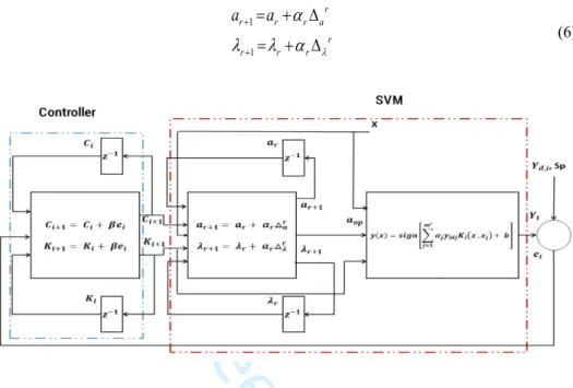
kernel function. SVM maps the non-linearly separable data into a higher-dimensional space by using kernels to make the data linearly separable. A simple representation of SVM in the form of control systems by using interior point methods is shown in Figure 1.
By using other methods for solving SVM’s QP problem, different models will be generated. Our work and representation of SVM is just an example for proving the idea that SVM can be assumed as a control system and can be assessed by intelligence and logical methods of control field. To find the SVM dynamic, equation (1) can be written in a matrix form as shown in equation (2). Then by using interior point method for solving equation (2) that is a QP problem, the dynamic of SVM arrives, as can be seen in Figure 1.
. (2) 1 2 . . 0 , & 0
max
T T a T a e a S a s t a a C a y where [ , , , ]1 2 T, is a 1*n vector, is a 1*n vector,
n
a K e[1,1, ,1]K T C[ , , , ]C C K C T
is labels of training points, , and n is the number of y 𝑆= [𝑟𝑖,𝑗] 𝑟𝑖,𝑗= 𝛼𝑖𝛼𝑗𝑦𝑖𝑦𝑗𝐾(𝑥𝑖,𝑥𝑗)
training points.
Then, the Lagrange function of (2) for a fixed value of the barrier parameter μ, can be written as shown in equation (3), and 𝐹𝜇(𝑎,𝜆)and 𝐽𝜇(𝑎,𝜆)are defined as (4) and (5), respectively. (3)
1
( , )
(log( ) log(
))
2
T T TL a
a e
a S a
a y
a
C a
(4) ( , ) (log( log( ))) ( , ) ( , ) T T T a T L a e a S y a C a a F a L a a y (5) 2 2 2 2 2 ( , ) ( , ) (log( ) log( )) ( , ) 0 ( , ) ( , ) T a T L a L a S a C a y a a a J a y L a L a a By solving the linear system of form 𝐽𝜇(𝑎,𝜆)𝑑= 𝐹𝜇(𝑎,𝜆). where 𝑑= (∆𝑟𝑎, ∆𝑟𝜆 ), and r is the iteration number. 𝑎𝑟+ 1and 𝜆𝑟+ 1are found as follows
10 11 12 13 14 15 16 17 18 19 20 21 22 23 24 25 26 27 28 29 30 31 32 33 34 35 36 37 38 39 40 41 42 43 44 45 46 47 48 49 50 51 52 53 54 55
For Peer Review
(6) 1 1 r r r r a r r r r a a
Fig. 1. SVM from control field of view. Controller is an iterative learning controller that is explained in section 4 and 5. Sp and 𝑦𝑑,𝑖 are the desired number of support vectors and labels, respectively, is training error, X is 𝑒𝑖 training set and z is shifting operator.
SVM finds optimum set of support vectors aop by iteratively solving the QP problem using the interior point method.
By studying SVM from a control point of view, it can be seen that the kernel function, its parameters and its regularization parameter are as inputs of SVM algorithm along with data, and the support vectors are the system’s output that algorithm finds them by using the inputs in the training mode. All the aforementioned parameters are of vital importance in SVM, because unwise selection of them will generate poor set of support vectors that causes an increase in test error and test time. It can be concluded that by using control methods, the inputs to the SVM algorithm can be found in a way that the desired performance and high accuracy is achieved. Moreover, both the soft margin and hard margin problems are control problems, because they are trying to face with error in different ways. In hard margin problems, a zero training error is desired, while in soft margin a non-zero but limited amount of error is acceptable and these two trends are done by defining some constraints in SVM. In control theory, there are a huge number of procedures for managing the error like using integral of absolute error or paying attention to the transient behavior of the error, besides its steady state behavior, while in SVM just steady state error is considered. Based on the Fig.1, for controlling the SVM system the controller can be chosen from a vast variety of control fields like, classical control (Jing &
10 11 12 13 14 15 16 17 18 19 20 21 22 23 24 25 26 27 28 29 30 31 32 33 34 35 36 37 38 39 40 41 42 43 44 45 46 47 48 49 50 51 52 53 54 55
For Peer Review
Cheng, 2012), robust control (Ning et al., 2019; Jing 2011), adaptive control, optimal control, nonlinear control and intelligent control for approaching the desired performance. In this work, iterative learning control (ILC), a branch of intelligence control, is used for finding the optimal kernel function. Since ILC is a method that is not model based and has a closed-loop procedure that brings robustness, it seems that it is a good choice for approaching at specified goals. Because the dynamic and model of datasets are unknown and SVM’s system is uncertain and complicate. In the next sections, after a brief introduction, ILC as a simple and non-model-based control strategy is used to optimize the kernel function and show the effectiveness of control methods.
3. Iterative Learning Control
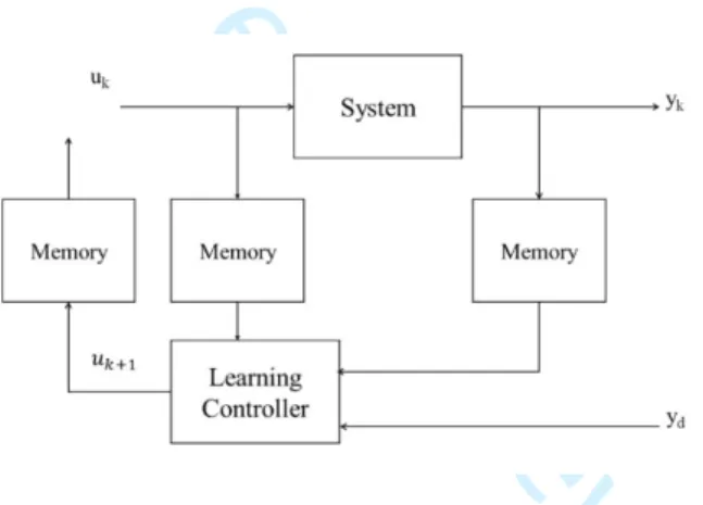
Control theory provides many methods to fulfil the needs of control systems. These techniques perform well when there is an accurate model for the control system. In the absence of the system model, various methods including Iterative Learning Control (ILC) methodology, which is a branch of intelligent control, can be used to efficiently control the system (Ahn et al., 2007). ILC systems have shown to perform well when the system model is uncertain and there is no information about nonlinearity of the system but the system deal with a repetitive task (Wang et al., 2009; Moore; Freeman et al., 2015). Figure 2 shows the building blocks of an ILC system. The ILC procedure based on the Figure 2 is as follows: At k-th iteration, input signal, , is applied to the system, system generates the 𝑢𝑘
output signal, . The resulting is stored in a memory. System computes the error signal, 𝑦𝑘 𝑦𝑘
, where , and use it in updating and constructing the new input signal, .
𝑒𝑘 𝑒𝑘=𝑦𝑘―𝑦𝑑 𝑢𝑘+ 1
It updates the input signal in a way that the error signal to be reduced iteratively and finally converges to zero. Various approaches can be used to update the input signal and improve the performance of the control system. In general input signal can be updated using:
Information from all previous iterations that called “higher-order in iteration”.
Information from the entire time duration of any previous iteration that called “higher-order in time”. Information up to time t-1 on the current iteration that called “current cycle
feedback”.
Any of these three approaches can be used to update the input signal without any limitations. However, for simplicity in this paper the third approach has been used. This approach uses error, , and the input signal, , to update the input signal, generating 𝑒𝑘 𝑢𝑘
as follows (Gunnarsson & Norrl¨of, 1997): 𝑢𝑘+ 1 (7) 1 , ( )[ ( ) ] k k k k d k k u H z u L z e e y y
where 𝐻(𝑧) is the filter function, 𝐿(𝑧) represents the learning function, z is the shift operator, β is the learning gain, k is the iteration number, , 𝑒𝑘 𝑦𝑑,𝑘and 𝑦𝑘are the tracking
10 11 12 13 14 15 16 17 18 19 20 21 22 23 24 25 26 27 28 29 30 31 32 33 34 35 36 37 38 39 40 41 42 43 44 45 46 47 48 49 50 51 52 53 54 55
For Peer Review
error, the desired output at iteration k and the system output at k-th iteration, respectively. The performance of an ILC system can be determined by having its learning and filter function. The filter helps to compensate the mismatches between the learning function and the system dynamic. However, if 𝐻(𝑧)≠1 the error never converges to zero. The learning, , and filter, , functions of an ILC system can both be non-causal and have the
𝐿(𝑧) 𝐻(𝑧) following form: (8) 2 1 2 22 21 00 11 12 2 1 2 22 21 00 11 12 ( ) ( ) H z z z z z L z l z l z l l z l z
L L L Lwhere 𝛼𝑖,𝑗and 𝑙𝑖,𝑗(∀ i=0,1,2,… and j=0,1,2,… ) are constant numbers that can be positive, negative or zero, and is the shift operator, that takes a function 𝑧𝛼 𝑖→𝑓𝑖 to its translation 𝑖→𝑓𝑖+𝛼. The application of this concept for the reduction of training error can lead to satisfactory algorithms.
Fig. 2. Block diagram of an iterative learning control configuration, where𝑢𝑘, and 𝑦𝑘 𝑦𝑑represent input, output and desired output signals in the k-th iteration, respectively (Ahn et al., 2007).
4. Proposed Algorithm
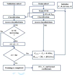
Figure 3 shows a block diagram of the proposed Iterative Learning Control based Support Vector Machine Kernel Optimization (ILC-SVMKO) method. The proposed method uses the following initialization parameters, which imperially found to be effective, to find optimal kernel function and regularization parameter: initial kernel function, K, is set to be a linear kernel function, regularization parameter, C, is set to 10, learning gain, β, is considered to be either a polynomial or Radial Basis Function (RBF) kernel, learning function, L(z), is considered to be a p-type, d-type or d2-type and the counter r1 is to a predefined value for each dataset. The proposed method first divides the input dataset into three subsets, train, validation and test subsets. The proposed method first trains the SVM
10 11 12 13 14 15 16 17 18 19 20 21 22 23 24 25 26 27 28 29 30 31 32 33 34 35 36 37 38 39 40 41 42 43 44 45 46 47 48 49 50 51 52 53 54 55
For Peer Review
using the training subset of the dataset, generating the Support Vectors (SVs) and their numbers (NSVs). The resulting SVs are then used to classify the train-and validation-data subsets. Resulting classified train and validation data are then used to calculate Training Error (TE) and Validation Error (VE), where the resulting TE is used to update the kernel function and its regularization parameter as it follows: It first checks if the value of r1 is below the predefined threshold value; If so, it updates the kernel function using equation 15, 16 or 17, based on the used learning function and the regularization parameter using equation 18; the resulting VE is used as a measure to determine the completion of the algorithm; it checks the resulting VE; if it is increasing, it adds one to r1 and updates the kernel function and its regularization parameter and proceeds with the algorithm until arrives at its predefined maximum number of iterations, which is allowed to reduce the VE. At this stage, the training stage of the algorithm is completed and the resulting SVs, kernel function and its regularization parameter are used to classify the test subset and calculating the algorithm’s classification accuracy. The theory behind the proposed algorithm is as follows:
The proposed ILC based algorithm uses the training error and the resulting number of support vectors information to update the kernel function and the regularization parameter, C, in a way that output error converges to zero. As mentioned in Section 2, various methods can be used to update the input signal, in this research the third mothed, as was explained in equation (8), is used to update the input signal, aiming to decreasing both number of SVs and TE. Therefor equation (8) can be rewritten as:
(9) 1 ( )[ ( ) ] i i i K H z K L z e (10) , , ( ) ( ) i i i d d i d i y Y x X y y e y x y x NS Sp
where 𝑌𝑖is set of predicted labels for misclassified training points in i-th iteration, while 𝑋𝑖and 𝑌𝑖𝑑 are set of their corresponding training points and desired labels, respectively. 𝑁𝑆𝑖 is number of support vectors in i-th iteration, Sp is the desired number of support vectors (presented results in this paper generated with Sp = 25), 𝑦𝑑(𝑥) is the desired label for data point, x and y(x) is the predicted class for that data point, and its function is as follows: (11) 1 ( ) ( , ) i m i ldj i j j y x sign
y K x x b
10 11 12 13 14 15 16 17 18 19 20 21 22 23 24 25 26 27 28 29 30 31 32 33 34 35 36 37 38 39 40 41 42 43 44 45 46 47 48 49 50 51 52 53 54 55For Peer Review
Fig. 3. Block diagram of the Iterative Learning Control based Support Vector Machine Kernel Optimization (ILC-SVMKO) method.
where 𝐾𝑖(𝑥,𝑥𝑗) is the kernel function in i-th iteration, 𝑚𝑖is the number of support vectors in i-th iteration, 𝛼𝑗are Lagrange coefficients, while 𝑥𝑗 and 𝑦𝑙𝑑𝑗are their corresponding support vectors and desired classes, respectively. As mentioned in (Phienthrakul & Kijsirikul, 2008), the function must satisfy Mercer’s condition, the filter function, H, the learning gain, β, the learning function, L, and the initial kernel, K0, should be chosen in a way to satisfy this condition. Consequently, Radial Basis Function (RBF) or polynomial kernels are used to determine learning gain for each input misclassified data, creating a linear weighting combination of kernels, where the weights are specified by the filter function and the learning function. The filter function is considered as H =1 to have the possibility of arriving at zero tracking error, as mentioned in Section 2. Due to the effect of learning function on speed of convergence, three types of learning functions, p-type, d-type and d2-d-type are considered, and the results are compared with each other in this research. The initial kernel acts as a prior knowledge about the structure of the data, so by having any information about data the initial kernel can be chosen from a wide variety of kernel functions. In this article, it is considered that there is no information about the structure of the data set, and the point that starting from complex kernel functions can increase the chance of over fitting. As the result, the proposed algorithm starts from the simplest kernel function named linear kernel and during training the complexity of kernel function increases by using ILC strategy in the way that explained in the rest. The error value was set to zero at the first iteration. By considering the learning function as p-type, d-type or d2-type based on equation (9), L(z) can be re-written respectively as:
10 11 12 13 14 15 16 17 18 19 20 21 22 23 24 25 26 27 28 29 30 31 32 33 34 35 36 37 38 39 40 41 42 43 44 45 46 47 48 49 50 51 52 53 54 55
For Peer Review
(12) 00 ( ) l z l (13) 1 00 11 ( ) L z l l z (14) 1 2 00 11 12 ( ) L z l l z l zwhere 𝑙00, 𝑙11and 𝑙12 are considered as 1. Substituting equation (12), (13), (14) and H(z) = 1 into (9) results in equations as follows, respectively
(15) 1 i i i K K e (16) 1 ( 1) i i i i K K e e (17) 1 ( 1 2) i i i i i K K e e e
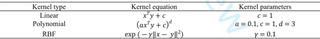
where K0 is considered as a linear kernel function and β is considered as a RBF or polynomial kernel. kernel types, their equations and parameters which are used to generate experimental results are tabulated in Table 1. From equations (15), (16) and (17), it can be seen that the resulting kernel is always a linear combination of some kernels.
As proven in (Shawe-Taylor & Cristianini, 2004), a linear combination of kernels is a kernel function, which can be used by the SVM algorithm. The regularization parameter, C, can then be updated using p-type learning function and Equation (9) can be re-written as:
(18)
1
i i i
C C e
C0 = 10, and β = 0.05 are used as the initial values in this research. Table 1. kernel types, their equations and parameters.
Kernel type Kernel equation Kernel parameters
Linear 𝑥𝑇𝑦+𝑐 𝑐= 1
Polynomial (𝑎𝑥𝑇𝑦+𝑐)𝑑 𝑎= 0.1, 𝑐= 1, 𝑑= 3
RBF exp (― 𝛾‖𝑥 ― 𝑦‖2) 𝛾= 0.1
5. Experimental Results
To assess the performance of the proposed Iterative Learning Control based Support Vector Machine Kernel Optimization (ILC-SVMKO), experimental results were generated using ten datasets from UCI machine learning repository called: Letter Recognition (LR) (letters ‘A’ and ‘N’ are used for this experiment), Wisconsin Breast Cancer (WBC), Liver Disorder (LD), Mnist (numbers ‘2’ and ‘8’ are used for this experiment), Diabetes, Heart Disease, Ionosphere, Parkinson, Iris and Sonar datasets. The number of instances and dimension of the datasets were used in this experiment are tabulated in Table 2, and these datasets are available in (Bren). 10 11 12 13 14 15 16 17 18 19 20 21 22 23 24 25 26 27 28 29 30 31 32 33 34 35 36 37 38 39 40 41 42 43 44 45 46 47 48 49 50 51 52 53 54 55
For Peer Review
Table 2. Datasets description. Dataset #Instances #Dimension
Letter 1536 17 Wbc 683 11 Liver disorder 346 7 MNIST 3850 6 Diabetes Sonar Heart Ionosphere Parkinson 804 208 303 351 400 8 60 75 34 22 Iris 150 4
To generate experimental results, all datasets were first normalized, and the datapoints in each dataset were randomly divided into three subsets: train-subset (70%), validation-subset (10%) and test-validation-subset (20%).
5.1. The proposed method vs. anchor SVM method
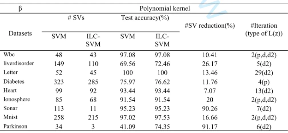
Experimental results for the proposed ILC-SVMKO and the anchor SVM using nine datasets were generated. Table 3 and 4 shows the resulting number of Support Vectors (#SVs) and the accuracy of the proposed ILC-SVMKO when using different type of learning functions and the anchor SVM for different datasets. From Table 3 and 4, it can be seen that the proposed technique generates superior performance to those of anchor SVM method in term of accuracy at significantly lower number of SVs when it uses a polynomial kernel; while it generates very competitive results in term of accuracy to those of anchor SVM method at significantly lower number of SVs when it uses the RBF kernel.
Table 3. Performance of the proposed ILC-SVMKO method versus anchor SVM method when
𝛽 is Polynomial kernel. β Polynomial kernel # SVs Test accuracy(%) Datasets SVM ILC-SVM SVM ILC-SVM #SV reduction(%) #Iteration (type of L(z)) Wbc 48 43 97.08 97.08 10.41 2(p,d,d2) liverdisorder 149 110 69.56 72.46 26.17 5(d2) Letter 52 45 100 100 13.46 29(d2) Diabetes 323 285 75.97 76.62 11.76 4(p) Heart 99 92 93.44 93.44 7.07 13(d2) Ionosphere 85 68 91.54 91.54 20 2(p,d,d2) Sonar 113 11 95.23 95.23 90.26 7(d2) Mnist 258 215 97.02 97.53 16.66 2(p,d,d2) Parkinson 34 3 41.09 74.35 91.17 6(d2) 10 11 12 13 14 15 16 17 18 19 20 21 22 23 24 25 26 27 28 29 30 31 32 33 34 35 36 37 38 39 40 41 42 43 44 45 46 47 48 49 50 51 52 53 54 55
For Peer Review
Table 4. Performance of the proposed ILC-SVMKO method versus anchor SVM method when
𝛽 is RBF kernel. β RBF kernel # SVs Test accuracy(%) Datasets SVM ILC-SVM SVM ILC-SVM #SV reduction(%) #Iteration (type of L(z)) Wbc 55 42 98.54 97.08 23.63 2(p,d,d2) liverdisorder 181 126 71.01 65.21 30.38 2(p,d,d2) Letter 131 70 100 100 46.56 2(p,d,d2) Diabetes 346 280 77.92 76.62 19.07 2(p,d.d2) Heart 120 106 91.80 93.44 11.66 2(p,d,d2) Ionosphere 177 135 98.59 98.59 23.72 2(p,d,d2) Sonar 149 112 92.85 92.85 24.83 3(p) Mnist 314 244 97.79 97.79 22.29 2(p,d,d2) Parkinson 140 118 82.05 79.48 15.71 3(d,d2)
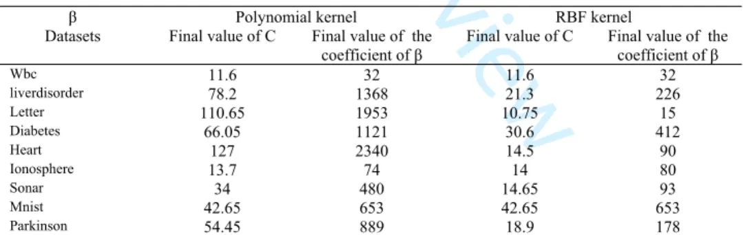
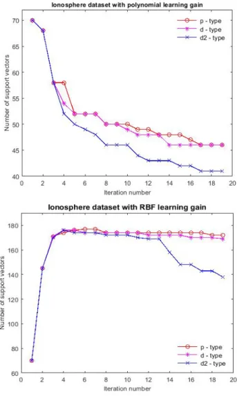
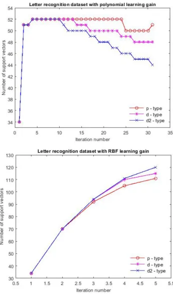
Figures 4 and 5 shows resulting number of SVs for Ionosphere and Letter datasets per iteration using polynomial and RBF kernels for p-type, d-type and d2-type learning functions. From these figures, it can be seen that the proposed technique when using d2-type learning function converges faster than when it uses either p-d2-type or d-d2-type learning functions. The achieved optimal value for regularization parameter, C, and learning gain, β, for training different datasets using the proposed ILC-SVMKO method are tabulated in Table 5.
Table 5. Resulting regularization parameter, C, and learning gain, β for different datasets using the proposed ILC_SVMKO method.
β Polynomial kernel RBF kernel
Datasets Final value of C Final value of the coefficient of β
Final value of C Final value of the coefficient of β Wbc 11.6 32 11.6 32 liverdisorder 78.2 1368 21.3 226 Letter 110.65 1953 10.75 15 Diabetes 66.05 1121 30.6 412 Heart 127 2340 14.5 90 Ionosphere 13.7 74 14 80 Sonar 34 480 14.65 93 Mnist 42.65 653 42.65 653 Parkinson 54.45 889 18.9 178 10 11 12 13 14 15 16 17 18 19 20 21 22 23 24 25 26 27 28 29 30 31 32 33 34 35 36 37 38 39 40 41 42 43 44 45 46 47 48 49 50 51 52 53 54 55
For Peer Review
Fig. 4. Resulting number of SVs for Ionosphere and Letter dataset per iteration using polynomial kernels for p-type, d-type and d2-type learning functions.
10 11 12 13 14 15 16 17 18 19 20 21 22 23 24 25 26 27 28 29 30 31 32 33 34 35 36 37 38 39 40 41 42 43 44 45 46 47 48 49 50 51 52 53 54 55
For Peer Review
Fig. 5. Resulting number of SVs for Ionosphere and Letter dataset per iteration using RBF kernels for p-type, d-type and d2-d-type learning function.
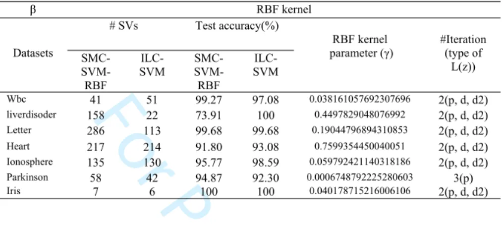
5.2. The proposed method vs. SMC-SVM-RBF method
In this part the performance of the proposed Iterative Learning Control based Support Vector Machine Kernel Optimization (ILC-SVMKO) is compared with SMC-SVM-RBF method (Yalsavar et al., 2019), using seven datasets. By this aim, first the optimal value of RBF kernel is found using SMC-SVM-RBF method, then the resulted parameter is used in ILC-SVMKO. Based on the results in Table 6 and 7, it can be seen that the proposed
10 11 12 13 14 15 16 17 18 19 20 21 22 23 24 25 26 27 28 29 30 31 32 33 34 35 36 37 38 39 40 41 42 43 44 45 46 47 48 49 50 51 52 53 54 55
For Peer Review
method gives either superior or very competitive results in terms of test accuracy and number of support vector to SMC-SVM-RBF method.
Table 6. Performance of the proposed ILC-SVMKO method versus SMC-SVM-RBF method when 𝛽 is RBF kernel. β RBF kernel # SVs Test accuracy(%) Datasets SMC- SVM-RBF ILC-SVM SMC- SVM-RBF ILC-SVM RBF kernel parameter (γ) #Iteration (type of L(z)) Wbc 41 51 99.27 97.08 0.038161057692307696 2(p, d, d2) liverdisoder 158 22 73.91 100 0.4497829048076992 2(p, d, d2) Letter 286 113 99.68 99.68 0.19044796894310853 2(p, d, d2) Heart 217 214 91.80 93.08 0.7599354450040051 2(p, d, d2) Ionosphere 135 130 95.77 98.59 0.059792421140318186 2(p, d, d2) Parkinson 58 42 94.87 92.30 0.0006748792225280603 3(p) Iris 7 6 100 100 0.040178715216006106 2(p, d, d2)
Table 7. Resulting regularization parameter, C, and learning gain, β for different datasets using the proposed ILC_SVMKO method.
β RBF kernel
Datasets Final value of C Final value of the coefficient of β Wbc 11.3 26 liverdisorder 10.95 19 Letter 10.75 15 Heart 14.95 99 Ionosphere 12.58 57 Parkinson 12.89 58 Iris 10.95 19 6. Conclusions
Since the main goal of control theory is to bring the behavior of the universe under the human’s control, it provides and suggests a huge number of logical and effective methods for dealing with different situations and approaching at diverse goals. As the control theory provides the ability of monitoring the behavior of systems in details and from different aspects, it is very useful to assess the behaivor of SVM from control view. Looking at SVM and its problems from control field of view enables us in controlling its behavior from both steady state and trasient aspects. Moreover, the SVM algorithm provides lots of beneficial information in its training phase that can be used in finding the correct inputs for the algorithm as ILC showed this point as a simple control method. The proposed method adapted the Iterative Learning Control (ILC) technique to optimize SVM’s kernel parameter. The performance of the proposed method was evaluated and compared with that of traditional SVM using nine benchmark datasets, and state-of-the-art
SMC-SVM-10 11 12 13 14 15 16 17 18 19 20 21 22 23 24 25 26 27 28 29 30 31 32 33 34 35 36 37 38 39 40 41 42 43 44 45 46 47 48 49 50 51 52 53 54 55
For Peer Review
RBF method using seven datasets. Experimental results show that the proposed techniques achieve higher performance to that of traditional SVM in term of accuracy at significantly lower number of SVs when using a polynomial kernel and generates very competitive results in term of accuracy to those of traditional SVM, and state-of-the-art SMC-SVM-RBF method at significantly lower number of SVs when using the SMC-SVM-RBF kernel. Moreover, since ILC is an un-model based, closed-loop strategy, its application does not narrow to SVM. By looking at the whole machine learning algorithms from a higher perspective and considering them as different systems with their own inputs and outputs, then ILC can play its significant rule as a controller for compensating and tuning different parameters in different machine learning frame works.
References
Abdiansah, A. and Wardoyo, R. Time complexity analysis of support vector machines (svm) in libsvm. International Journal of Computer Applications, pp. 0975 - 8887, 2015.
Ahn, H., Chen, Y., and Moore, K. L. Iterative learning control: Brief survey and categorization. IEEE Transactions on Systems, Man, and Cybernetics, Part C (Applications and Reviews), 37(6):1099 – 1121, 2007.
Auria, L. and Moro, R. A. Support vector machines (svm) as a technique for solvency analysis. SSRN Electronic Journal, 2008.
Bren, D. http://www.ics.uci.edu/ mlearn/MLRepository.html. Accessed: 2019-May-12. Champaigne, J. https://www.electronics-inc.com/wpcontent/uploads/BenefitsOfClosedLoop.pdf. Accessed: 2019-Augest-10.
Chapelle, O., Vapnik, V., Bousquet, O., and Mukherjee, S. Choosing multiple parameters for support vector machines. Machine Learning, 46(1-3):131–159, 2002.
Chen, Z. M., ZHAO, Q., WANG, Z., SHAO, X., and WEN, X. Sliding mode control based on svm for fractional order time-delay system. In International Conference on Control and Automation. IEEE, 2016.
Chung, K., Kao, W., Sun, T., Wang, L., and Lin, C. Radius margin bounds for support vector machines with the rbf kernel. In Neural Computation, 2003.
Demyanov, S., Bailey, J., Ramamohanarao, K., and Leckie, C. Aic and bic based approaches for svm parameter value estimation with rbf kernels. In Langley, P. (ed.), Asian Conference on Machine Learning, pp. 97–112, 2012.
Diosan, L., Oltean, M., Rogozan, A., and Pecuchet, J. Improving svm performance using a linear combination of kernels. In International Conference on Adaptive and Natural Computing Algorithms, Berlin, 2007. Springer.
Downs, T., Gates, K. E., and Masters, A. Exact simplificationof support vector solutions. Journal of Machine Learning Research, 2:293–297, 2001.
Famouri, M., Taheri, M., and Azimifar, Z. Support vector machines and machine learning on documents. International Journal of Pattern Recognition and Artificial Intelligence, 29(8):155– 1013, 2015. 10 11 12 13 14 15 16 17 18 19 20 21 22 23 24 25 26 27 28 29 30 31 32 33 34 35 36 37 38 39 40 41 42 43 44 45 46 47 48 49 50 51 52 53 54 55
For Peer Review
Freeman, C. T., Rogers, E., Burridge, J. H., Hughes, A., and Meadmore, K. L. (eds.). Iterative learning control for electrical stimulation and stroke rehabilitation. Springer, 2015.
Geebelen, D., Suykens, J. A. K., and Vandewalle, J. Reducing the number of support vectors of svm classifiers using the smoothed separable case approximation. In IEEE Transactions on Neural Networks and Learning Systems, 2012.
Georgevici, A. I. and Terblanche, M. Neural networks and deep learning: a brief introduction.
Intensive Care Medicine, 45(5):712—-714, 2019.
Gou, J., Ma, H., Ou, W., Zeng, S., Rao, Y., and Yang, H. A generalized mean distance-based k-nearest neighbor classifier. Expert Systems with Applications, 115:356–372, 2019.
Gunnarsson, S. and Norrl¨of, M. A short introduction to iterative learning control. Link¨oping University Electronic Press, 1997.
Han, T., Jiang, D., and Wang, L. Comparison of ran-dom forest, artificial neural networks and support vectormachine for intelligent diagnosis of rotating machinery.Transactions of the Institute of Measurement and Control,48(8):2681–2693, 2018.
Imbault, F. and Lebart, K. A stochastic optimization approach for parameter tuning of support vector machines. In Proceedings of the 17th International Conference on Pattern Recognition. IEEE, 2004. Jing, X. An h control approach to robust learning of feedfor-ward neural networks.Neural networks, 24(7):759–766,2011.
Jing, X. and Cheng, L. An optimal pid control algorithm fortraining feedforward neural networks.IEEE Transactionson Industrial Electronics, 60(6):2273–22834, 2012.
Joachims, T. Text categorization with support vector machines: Learning with many relevant features. In European Conference on Machine Learning. Springer, 1998.
Keerthi, S. S. Efficient tuning of svm hyperparameters using radius/margin bound and iterative algorithms. In IEEE Transactions on Neural Networks, 2002.
Li, C., Ho, H., Liu, Y., and Lin, C. An automatic method for selecting the parameter of the normalized kernel function to support vector machines. Information science and engineering, 28:1–15, 2012. Li, Y., Zhang, W., and Lin, C. Simplify support vector machines by iterative learning. Neural Information Processing - Letters and Reviews, 10(1), 2006.
Liao, P., Zhang, X., and Li, K. Parameter optimization for support vector machine based on nested genetic algorithms. Journal of Automation and Control Engineering, 4(1):78–83, 2016.
Liu, S., Jia, C., and Ma, H. New weighted support vector machine with ga-based parameter selection. In Proceedings of the 17th International Conference on Pattern Recognition, IEEE.Guangzhou, 2005.
Liu, Z. and Xu, H. Kernel parameter selection for support vector machine classification. Journal of Algorithms Computational Technology, 8(2), 2013.
Manning, C. D., Raghavan, P., and Schutze, H. Support vector machines and machine learning on documents. Introduction to Information Retrieval, pp. 293–320, 2009.
Moore, K. Iterative learningcontrol. http://inside.mines.edu/ kmoore/survey.pdf. Accessed: 2019-March-17.
Nguyen, D. and Ho, T. An efficient method for simplifying support vector machines. International Conference on Machine Learning, Bonn, 2005.
10 11 12 13 14 15 16 17 18 19 20 21 22 23 24 25 26 27 28 29 30 31 32 33 34 35 36 37 38 39 40 41 42 43 44 45 46 47 48 49 50 51 52 53 54 55
For Peer Review
Ning, H., Qing, G., Tian, T., and Jing, X. Online iden-tification of nonlinear stochastic spatiotemporal systemwith multiplicative noise by robust optimal control-basedkernel learning method.IEEE Transactions on NeuralNetwork Learning System, 2(30):389–404, 2019.
Osuna, E. and Gerosi, F. Reducing the run-time complexity of support vector machines. In International Conference on Pattern Recognition, 1998.
Osuna, E., Freund, R., and Girosit, F. Training support vector machines: an application to face detection. San Juan, 1997. IEEE.
Phienthrakul, T. and Kijsirikul, B. Adaptive stabilized multirbf kernel for support vector regression. In IEEE International Joint Conference on Neural Networks (IEEE World Congress on Computational Intelligence), Hong Kong, 2008. IEEE.
Rojas, S. A. and Reyes, D. F. Adapting multiple kernel parameters for support vector machines using genetic algorithms. In IEEE Congress on Evolutionary Computation, Edinburgh, 2005. IEEE. Shawe-Taylor, J. and Cristianini, N. (eds.). Kernel methods for pattern analysis. Cambridge university press, 2004.
Shen, X. and Gu, Y. Nonconvex sparse logistic regression with weakly convex regularization. In
IEEE Transactions on Signal Processing. IEEE, 2018.
Shi, H., Xiao, H., Zhou, J., and Li, N. Radial basis function kernel parameter optimization algorithm in support vector machine based on segmented dichotomy. In The 2018 5th International Conference on Systems and Informatics, Nanjing, 2018. IEEE.
Staelin, C. Parameter selection for support vector machines. In The 2018 5th International Conference on Systems and Informatics, Technion, 2002.
Suykens, J., Vandewalle, J., and Moor, B. D. Optimal control by least squares support vector machines. Neural Networks, 14(1):23–35, 2001.
Tang, Y., Guo, W., and Gao, J. Efficient model selection for support vector machine with gaussian kernel function. In Symposium on Computational Intelligence and Data Mining, Nashville, 2009. IEEE.
Tsouros, D. C., Smyrlis, P. N., and Tsipouras, M. G. Random forests with stochastic induction of decision trees. In IEEE 30th International Conference on Tools with Artificial Intelligence, Volos, 2018. IEEE.
Wang, L. and Chan, K. L. Learning kernel parameters by using class separability measure. In Neural Information Processing Systems, Vancouver, 2002. NIPS.
Wang, Y., Gao, F., and Doyle, F. J. Survey on iterative learning control, repetitive control, and run-to-run control. Journal of Process Control, 19(10):1589–1600, 2009.
Wu, K. and Wang, S. Choosing the kernel parameters of support vector machines according to the inter-cluster distance. In International Joint Conference on Neural Network Proceedings, Vancouver, 2006. IEEE.
Xia, X., Lyu, M. R., Lok, T., and Huang, G.-B. Methods of decreasing the number of support vectors via k –mean clustering. In International Conference on Intelligent Computing, Verlag, 2005. Springer.
Xia, Y., nad Y. Li, C. L., and Liu, N. A boosted decision tree approach using bayesian hyper-parameter optimization for credit scoring. Expert Systems with Applications, 78: 225-241, 2017.
10 11 12 13 14 15 16 17 18 19 20 21 22 23 24 25 26 27 28 29 30 31 32 33 34 35 36 37 38 39 40 41 42 43 44 45 46 47 48 49 50 51 52 53 54 55
For Peer Review
Xie, T., Yao, J., and Zhou, Z. Da-based parameter optimization of combined kernel support vector machine for cancer diagnosis. Processes, 7(5):263, 2019.
Xuefeng, L. and Fang, L. Choosing multiple parameters for svm based on genetic algorithm. In 6th International Conference on Signal Processing, Beijing, 2002.
Yalsavar, M., KArimaghaee, P., SHeikh-Akbari, A.,J.Dehmeshki, Khooban, M. H., and Al-Majeed, S. Slid-ing mode control based support vector machine rbf kernelparameter optimization. InIEEE International Confer-ence on Imaging Systems Techniques, 8-10 December2019), Abu Dabi, UAE, 2019. IEEE.
Yin, S. and Yin, J. Tuning kernel parameters for svm based on expected square distance ratio.
Information Sciences, pp. 92–102, 2016.
Zhang, D., Chen, S., and Zhou, Z.-H. Learning the kernel parameters in kernel minimum distance classifier. Pattren Recognition, 39(1):133–135, 2006.
10 11 12 13 14 15 16 17 18 19 20 21 22 23 24 25 26 27 28 29 30 31 32 33 34 35 36 37 38 39 40 41 42 43 44 45 46 47 48 49 50 51 52 53 54 55
For Peer Review
Maryam Yalsavar
received her B.Sc. and M.Sc. (Hons.) degrees in Control Engineering from Shiraz University, Shiraz, Iran. Currently, she is conducting researches towards causal machine learning at Shiraz University. She is interested in making connections between different fields of knowledge to improve their performance and reduce their problems specially in fields of machine learning.
Paknoosh Karimaghaei was born in Shiraz, Iran in 1967. He received his B.Sc. (Hons.) in electrical engineering from Shiraz University in 1986. Followed by his M.Sc. (Distinction), and Ph.D. degrees in electronic and electrical engineering, 1995, and 2001, respectively from the Amir Kabir University of Tehran. In 2008, he became an assistant professor in the Shiraz University and then associate Professor in 2014. His research looks at instrumentation, nonlinear control systems, and control theories.
Akbar Sheikh-Akbari
received the B.Sc. (Hons.), M.Sc. (Distinction), and Ph.D. degrees in electronic and electrical engineering, 1992, 1995, and 2005, respectively. After completing the Ph.D. degree at the University of Strathclyde in the field of stereo/multiview video processing, he continued his career in industry, worked on real-time embedded video analytics systems. He is currently an Associated professor (Reader) in the School of Computing, Creative Technologies & Engineering, Leeds Beckett University. His research interests include, source camera identification, standard and non-standard image/video codecs, e.g., H.264 and HEVC, multi-view image/video processing, biometric identification techniques, e.g. ear and iris recognition, color constancy adjustment techniques, resolution enhancement methods, edge detection in low-SNR environments, and medical image processing, compressive sensing, hyperspectral image processing, camera tracking using retro-reflective materials, assisted living technologies, video analytics and machine learning. He has published more than 100 articles in international journals and conferences.
Pancham Shukla received his BE in Electronic Engineering (1995) and ME in Electronic and Computer Engineering (2001) from BVM Engineering College, Sardar Patel University, India. He received his MPhil in Electronic and Electrical Engineering (2003) from Strathclyde University, UK and PhD in Electrical and Electronic Engineering (2007) from Imperial College London. Dr Pancham Shukla held various academic and research positions in India and UK since 1996. He has been with London Metropolitan University since 2007. Currently he is a Senior Lecturer and a Course Leader in School of Computing and Digital Media. Dr Shukla is a recipient of Vice Chancellor’s award for outstanding contribution to Learning and Teaching as well as Student Union’s award as an outstanding member of academic staff. His research interest broadly spans the field of Communications, Signal and Image processing. He has organized conferences and served as a technical session chair along with reviewing many international conference and journal papers.
Peyman Setoodeh
received the B.Sc. and
10 11 12 13 14 15 16 17 18 19 20 21 22 23 24 25 26 27 28 29 30 31 32 33 34 35 36 37 38 39 40 41 42 43 44 45 46 47 48 49 50 51 52 53 54 55
For Peer Review
M.Sc. degrees (Hons.) in electrical engineering from Shiraz University, Shiraz, Iran, and the Ph.D. degree incomputational engineering and science from McMaster University, Hamilton, ON, Canada. He is currently an Assistant Professor with the School of Electrical and Computer Engineering, Shiraz University.Previously, he was a Senior Engineer with Huawei Technologies Canada and a Principal Research Engineer with McMaster University. He has co-authored a book on Cognitive Radio and a paper on Cognitive Control, which was featured as a cover story in the December 2012 issue of PROCEEDINGS OF THE IEEE. His research interests include cognitive systems, quantum control, and artificial intelligence. He was arecipient of the Monbukagakusho Scholarship from the Ministry of Education, Culture, Sports, Science, and Technology, Japan.
10 11 12 13 14 15 16 17 18 19 20 21 22 23 24 25 26 27 28 29 30 31 32 33 34 35 36 37 38 39 40 41 42 43 44 45 46 47 48 49 50 51 52 53 54 55