Classification and Feature Selection Approaches for
Cardiotocography by Machine Learning
Techniques
Satish Chandra Reddy Nandipati and Chew XinYing
School of Computer Sciences, 11800, Universiti Sains Malaysia, Pulau Pinang, Malaysia. [email protected]
Abstract— Cardiotocography (CTG) is the commonly used tool to monitor fetal distress (hypoxia), other fetal risks such as fetal heart rate, and autonomous nervous system maturation. If not rectified in the early stages, these problems may lead to fetal death. Thus, it is important to know which selected features are necessary to predict the risk. The objective of this research is to carry out the classification model and feature selection on the derived dataset with R-based CARET and Python-based Scikit learn packages. Despite different analytical techniques used, it is observed that the nature of the tools may play a role in model classification on the given dataset. The classification accuracies of the dataset are found to be similar when compared with the UCI repository CTG dataset. The similar performance of accuracies has been noticed in the random forest and naive Bayes, and average accuracy with respect to complete features (R-based machine learning techniques). On the other hand, the selected features showed classification accuracies with similar performance in naïve Bayes, bagging and boosting (Python-based machine learning techniques). However, the study found that correlated features contributed to the increase of classification accuracy of complete features. The selected features show the accuracies similar to the complete dataset indicating as these features play a role in the prediction of CTG data.
Index Terms—Classification; Feature Selection; Machine Learning; Python; R.
I. INTRODUCTION
The fetal scalp blood sampling (FBS) and cardiotocography (CTG) are the commonly used tools to monitor the fetal distress or any other common fetal risks, such as a change of fetal heart rate (FHR, acceleration or deceleration of FHR), and fetal movements, which may occur during pregnancy or before delivery [1, 2]. It also helps to search for predominant risk factors, such as the external stimuli, autonomous nervous system maturation, and detect the signs of fetal distress or intrapartum hypoxia/early signs of hypoxia [3]. Fetal distress is a progressive condition, where initially the foetus reacts at the onset of asphyxia (by an obstruction or injury of airway passages) with various compensatory mechanisms. Later, asphyxia may extend to the condition hypoxia, the altered hypoxia (inadequate delivery or utilization of oxygen by the body's tissues) leads to the changes in fetal physiology. If it is not rectified in the early stages, it may lead to an increased chances of brain damage or fetal death [4, 5]. The device used to perform the monitoring of FHR and uterine contraction (UC) is called an electronic fetal monitor (EFM) or cardiogram. The method of CTG involves the placement of two transducers onto the abdomen of a pregnant woman who
is typically in their third trimester to evaluate the maternal and fetal well-being. One transducer records the FHR and the other transducer monitors the UC using the ultrasound. Transducers may be either external or internal, the internal transducers refer to monitoring when an electronic transducer is connected directly to the fetal scalp, whereas the external measurement means strapping the two transducers to the abdominal wall. The tensions created in the maternal abdominal wall are used as a measure by CTG, providing an indirect indication of intrauterine pressure. The measure is represented by a time-scaled printed running paper from the cardiotocograph machine, which in turn is interpreted by experienced clinicians followed by the international guidelines. However, it is known that the assessment is not consistent due to the difference between the same and different clinicians respectively [6]. On the other hand, it was reported that more than 50% of deaths are due to the inability to recognize abnormal FHR patterns, and the lack of appropriate action [7]. Based on the published article, it is reported that sensitivity and specificity vary from 2 to 100% and 37 to 100% respectively [8].
On the other hand, the aforementioned clinical decisions made by doctors show there could be a possibility of human mistake, sensitivity, and specificity of the results, and leaving the hidden quality from the data, which leads to the death of the fetus. The improvement in the patient’s outcome and safety can be overcome by the decrease in medical errors and unwanted practice variation, which can be achieved by the integration of computer-based patient records and clinical decision support. Thus, the use of data mining algorithms on the medical dataset of CTG can be used for the accurate prediction of FHR and UC patterns. In this paper, our objectives are to compare the performance of R and Python tools, to build a better machine learning model and to know which feature selection attributes play a key role in the prediction of derived CTG dataset (which is randomly derived from UCI machine learning repository CTG dataset) with R and Python tools.
II. LITERATURE REVIEW
The process of exploring new and valuable information from the data is called data mining. This plays an important role in the intelligent medical system since it contributes to improving the quality of clinical decisions. Data mining consists of various disciplines. Among them machine learning is one of the disciplines and consists of different techniques, such as classification, regression in supervised
learning, clustering and association analysis in unsupervised learning [9]. For classification, the output is a categorical variable and the aim is to predict a class label from a set of classes based on instances/samples. The availability of the data due to the advances in modern obstetric practice has made it possible to perform robust and reliable machine learning techniques in classifying CTG patterns. The various classification machine learning (ML) algorithms used for the prediction of CTG patterns are reviewed below:
A. K-Nearest Neighbor’s Algorithm (KNN)
It is a simple classifier, easy to implement and understand, and it requires short training time. The whole training set is used for prediction and it cannot handle noises. The K-Nearest Neighbors (KNN) has been used for the prediction of cardiotocograph data (1831 instances with 21 attributes using (WEKA). The eight different machine learning algorithms have been used to study antepartum cardiotocography. Among the eight algorithms that used the highest accuracy is achieved by both k-NN (98.4%) and RF (99.18%) respectively, indicating that these classifications will be used to classify as normal or pathological [10]. A similar study with the feature selection technique, such as binary particle swarm optimization (PSO) along with K-NN has been used for the classification of fetal heart signals prediction, where it shows 83.8% accuracy, which is higher than 77.5% of SVM [11].
B. Support Vector Machine (SVM)
The support vector classifiers, based on kernel functions are divided into different types, which are linear, nonlinear, polynomial, radial basis function (RBF) and sigmoid. The support vector or data points are separated by the hyperplane or support vector machine. Some of the studies of SVM are as follows: The seven features have been extracted from the cardiotocography dataset obtained from the UCI Machine Learning Repository using the K-means algorithm. Later, these selected features were used to train the data with 10-fold cross-validation, and the accuracy is found to be 90.64%. The study shows that the K-SVM algorithm has the ability to classify the CTG dataset into normal, suspicious, or pathologic classes [12]. The comparative study with SVM and decision tree on a similar dataset showed an accuracy of 97.93 % and 97.41% respectively, with good precision and recall [13].
C. Random Forest (RF)
Random forest is a combination of multiple decision trees at training time, and the class prediction is based on the majority vote for classification. The cardiotocography dataset (2126 instances with 21 features) from UCI Machine Learning Repository has been used to classify three classes of CTG dataset (normal, suspicious and pathological) using a random forest classifier. An accuracy (93.6%) is noticed in both the complete and seven selected features such as AC, UC, ASTV, MSTV, ALTV, MLTV and Mean of Histogram [14]. A similar dataset has been evaluated (for normal and pathological classes) using J48, REPTree and random forest with bagging approach. For the selection of relevant features, the correlation feature selection - subset evaluation (cfs) method was used. The seven most relevant features found are AC, DS, DP, ASTV, MSTV, ALTV and Mean. The three classifiers accuracies for complete features have been almost similar to a slight variation in the random forest (94.7%), a
similar pattern was noticed with respect to reduced features. This indicates that relevant features, the random classifier with a bagging approach can be used for better classification of CTG data [15].
D. Naïve Bayes (NB)
Naïve Bayes assumes the probability of the features which are independent of each other, in which this classifier is based on Bayes. The different classification algorithms J48, JRIP, Naïve Bayes, Random forest, MLP and classification via regression have been used on the CTG dataset by using 2126 instances with 21 features. The Naïve Bayes showed an accuracy of 82.32% using the Weka tool [16]. In another study, the same dataset and Weka tool have been used for the prediction of FHR using Radial Basis Function, Decision Tree, Naive Bayes, and Multi-Layer Perceptron. Using Weka software and Naïve Bayes, the complete features showed 82.1% accuracy, whereas with 15 reduced features, the accuracy is 83.9% [17].
E. Neural Network (NN)
The neural network also called an artificial neural network, is inspired by the biological neural network that constitutes in the brain or central nervous system. The input layer, hidden layer, and output layer are the three major parts of the neural network. The different classification algorithms (extreme learning machine, radial basis function, random forest, support vector machine, and artificial neural network) have been used to know the most efficient machine learning technique to classify fetal heart rate. The sensitivity and specificity have been found to be greater than 88%, indicating all the used algorithms produced satisfactory results. However, the most significant results are produced by an artificial neural network with the sensitivity (99.73%) and specificity of 97.94% respectively [18]. In another study, four algorithms have been used, which are the SVM and RF as a control group, whereas convolution neural network classification method named “MKNet” and recurrent neural network named “MKRNN” as the experimental group. The real-time diagnosis of FHR data can be applied through experimental algorithms, in which it will learn directly from the FHR data. Based on the comparisons of the aforementioned algorithms, the speed and accuracy have been calculated. The speed results for RF are (14.35seconds) > SVM (118.90s) > MKNet (1330s = 19s∗70epoch) > MKRNN (350s = 5s∗70epoch), whereas the accuracy are for MKNet-C (94.70) > MKRNN (90.30) > RF (84.50) > SVM (83.46%). Based on the above results, it is confirmed that MKNet is the best algorithm for real-time FHR signal classification, indicating the neural network is a feasible and innovative model for fetal heart rate monitoring classification for real-time diagnosis [19].
F. Bagging and Boosting (B&B)
The bagging and boosting come under the ensemble techniques, in which a set of weak learners are combined to form a strong learner for better performance. Bagging is also called as bootstrap aggregating, in which random sampling takes place with replacement. This Machine learning technique is used for classification and regression analysis. It also reduces variance and avoids overfitting, whereas boosting is based on the weighted averages to make weak learners into stronger learners: It is useful to reduce bias and variance.
The CTG dataset (2126 samples and 21 features) were used to select the relevant features based on the Principal Component Analysis (PCA). Later, the data is trained and tested with the Adaptive Boosting (AdaBoost) algorithm integrated with Support Vector Machine (SVM) for the classification and prediction of fetal state. The overall classification accuracy of total and selected features is found to be 93 and 98.6% respectively with a computation time of 11.6s and 2.4s [20]. In another study, the decision tree-based AdaBoost has been used to determine the fetal distress, and it was found an accuracy of 95.01%, 0.034 MAE and 0.861 kappa statistics, indicating better performance can be seen through ensemble machine learning approach [21].
G. Feature Selection Approaches
The increase in diagnosis cost and the huge volume of data produced by different sources consist of the number of attributes. All attributes may not be useful, thus it is necessary to remove them during data preprocessing or feature selection. The feature selected attributes would, in turn, improve the performance to build a better classification. The various feature selection methods such as embedded, ensemble and hybrid methods, filter methods and wrapper methods have been applied to study the fetal heart rate or CTG analysis.
The 4 feature selection methods have been applied (Correlation-based Feature Selection, Symmetrical Uncertainty, ReliefF, Information Gain, Chi-Square feature selection methods), and 4 classification algorithms such as Jrip (Rule-based), J48 (Tree-based), KNN (Lazy Learner), NB (Bayes Learner) with WEKA tool have been used for Enhancing the Cardiotocography Classification Performance. The 4 feature selection methods showed different best selected features. The accuracy was found to be in a range of 86.78% to 98.73 % [22].
The influence of the 4 selected features methods such as Correlation-based, ReliefF, Information Gain, and Mutual Information on the performance of the Naïve Bayes for FHR patterns and fetal states have been performed. Among the 4 selected features, the ReliefF showed a better performance with an accuracy of 93.97% for fetal state classification [23]. In another study, the classification of cesarean section and normal vaginal deliveries using fetal heart rate signals have been studied with respect to random forest classifier and Recursive Feature Elimination (RFE). The random forest using all features from SMOTHE data shows specificity and sensitivity of 93% and 92% respectively. Similarly, the random forest using RFE fromSMOTE data showed 90.79% and 91.35% respectively [24].
III. DATA SOURCES
The publicly UCI machine learning repository has been used to retrieve the Cardiotocography (CTG) dataset
available at
https://archive.ics.uci.edu/ml/datasets/Cardiotocography. The multivariate datatype consists of 2126 instances with 23 attributes, which are numeric. The class attribute consists of 3 distinct values, which are Normal, Suspect, and Pathologic. The frequencies of 2126 instances are as follows: 1655 normal, 295 suspicious, and 176 pathologic, indicating the uneven distribution of the observations across the classes, which refers to class imbalance dataset.
The imbalanced datasets require special attention because
the regular classifiers accuracies are inappropriate to use for class imbalance [25], since these classifiers generally favor the majority class i.e., the class with a large number of instances. The performance of the classifier can be improved by the ensemble of classifiers. However, the majority of ensembles are static and cannot be applied to imbalanced datasets [26]. Apart from this, based on experimental results, it is known that the performance on the balanced dataset is better than the imbalance dataset [27]. In the view of aforementioned sentences, the dataset used in this study consists of 300 normal fetal state class randomly derived from 1655 instances from UCI repository CTG dataset), keeping other class codes as the same (i.e., 295 suspicious and 176 pathologic) with 23 attributes is shown in Table 1.
Table 1
Characteristics of CTG Dataset Used in This Study UCI Machine Learning
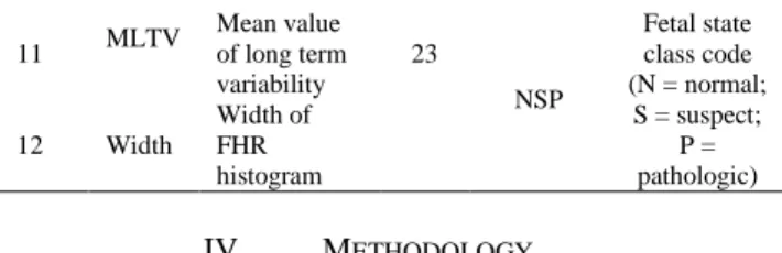
Repository Derived Dataset Attributes 23 23 Normal 1655 300 Suspicious 295 295 Pathologic 176 176 Total Instances 2126 771 A. Attributes Description
The dataset consists of 23 attributes. The predictable attribute is referred to “NSP: Fetal state class code (N = normal; S = suspect; P = pathologic)” remaining 22 as input attributes. The description of the attributes is shown in Table 2.
Table 2
Description of Attributes in the Dataset
S.No Code Description S.No Code Description
1 LB FHR baseline (beats per minute) 13 Min Minimum of FHR histogram 2 AC Accelerations
per second 14 Max
Maximum of FHR histogram 3 FM Fetal movements per second 15 Nmax Histogram peaks 4 UC Uterine contractions per second 16 Nzeros Histogram zeros 5 DL Light decelerations per second 17 Mod Histogram mode 6 DS Severe decelerations per second
18 Mean Histogram mean
7 DP Prolonged decelerations per second 19 Median Histogram median 8 ASTV Percentage of time with abnormal short term variability 20 Variance Histogram variance 9 MSTV Mean value of short term variability 21 Tendency Histogram tendency 10 ALTV Percentage of time with abnormal long term variability 22 CLASS FHR pattern class code (1 to 10)
11 MLTV Mean value of long term variability 23 NSP Fetal state class code (N = normal; S = suspect; P = pathologic) 12 Width Width of FHR histogram IV. METHODOLOGY A. Data Preprocessing
In the data preprocessing stage, missing values are not found in the dataset. The presence of different measuring units in the dataset need to be rescaled (i.e., the variable values between 0 and 1) using normalization. Thus, the normalization method is included in both R and Python machine learning techniques during the model building.
B. Data Analysis
The derived dataset consists of 771 instances with 23 attributes (Table 1) has been taken into consideration to build a classification model after normalization of the data. The R-based CARET package and Python-R-based Scikit learn was used as an analytical tool. A total of seven machine learning (ML) techniques, each (refer to literature review) was used to evaluate the performance of the classifiers and tools. Later, feature selection was also implemented on the aforementioned dataset.
In R-based caret package, the derived dataset with a percentage split of 70–30% was used as a training and testing data respectively with set.seed (123). The pre-processing steps such as normalization [(normalize <- function(x) {return ((x - min (x)) / (max(x) - min(x)))}], data splitting, and classification algorithms were carried out in R-based CARET package (https://cran.r-project.org/web/packages/). The five classification algorithms such as K-Nearest Neighbor (KNN, library “caret”, method = 'knn', tuneLength = 10), Support Vector Machine (SVM, library “caret”, method = 'svmLinear', tuneLength =10), Random Forest (RF, library “randomForest”, method= ‘rf’, ntree=500, importance=TRUE), Naïve Bayes (NB, library “e1071”, method = ‘naïve_bayes’) and Neural Network (NN, library “nnet”, method = 'nnet', trace= FALSE) and two ensemble classifiers such as bagging (library “adabag”, method = ‘treebag’) and boosting (library “gbm”, method= ‘gbm’, verbose=FALSE) with 10 fold cross validation (method = "cv", number = 10), were evaluated based on the aforementioned training and testing data.
The different feature selections methods such as correlation matrix (library “mblench”), recursive feature elimination (RFE) method with random forest algorithm (library “mblench”, functions = rfFuncs, method="cv", number=10; RFE-RF). The rank feature by Importance (library “class” and “mblench”) with the SVMpoly model (RFI-SVMpoly) is addressed using the CARET package in the R tool (http://topepo.github.io/caret/index.html).
In Python-based scikit learn package, the pre-processing steps such as normalization [preprocessing.normalize(X)], data splitting (70–30%), and the machine learning techniques with default values parameter settings available in open source by scikit-learn have been used to evaluate the classification performance on CTG dataset with set seed =7 and 10 fold cross-validation (n_splits=10, random_state=seed). The five classification algorithms version used are the KNeighborsClassifier, SVC (for SVM), RandomForestClassifier, Gaussian Naive Bayes (GNB),
MLPClassifier (for NN), and two ensemble classifiers such as the BaggingClassifier and GradientBoostingClassifier.
The feature selections methods such as correlation matrix (library “pandas”), recursive feature elimination (RFE) method with Logistic Regression model (RFE-LR) and the SelectKBest(score_func=f_classif,k=3;SelectKBest/f_classif ) were used from Scikit learn package in Python [28, 29]. The performance of a model on test data was calculated by accuracy, precision and recall in R and Python tool. Precision and recall measures the true positives (risk class) and the true negatives (normal class) respectively. Thus, the predictive capabilities of the classifiers can be measured by precision and recall values. The flow diagram, which represents the overall work process (methodology) is shown in Figure 1.
Figure 1: Flow diagram of methodology
V. RESULTS
A. Performance Comparison of R and Python ML Techniques on Derived Dataset
To the best of author knowledge, most of the classification model studies have been carried out on the UCI machine learning repository CTG dataset [14, 30]. Thus, there were no studies addressing the derived dataset with the seven machine learning techniques. Moreover, R and Python tools were selected to compare and understand which classification model and tool have a better performance on the dataset. To measure the performance of each classification algorithm, the accuracy has been taken into accordance.
The highest accuracy with similar performance of the classification algorithms (97.87%) has been observed both in the random forest and naïve Bayes followed by SVM and KNN (94.62% and 91.47 %), and similar performance of accuracy also been noticed in NN, bagging and boosting (86.19%) in R-ML techniques respectively. Whereas, this scenario is different in ‘Python’, in which boosting shows the highest accuracy (96.98%) followed by bagging (96.12%) and random forest (94.39%), apart from these remaining classifiers did not show similar accuracy performance (Table
3). In comparison to both the R and Python, ‘R’ shows the highest average accuracies (91.48%) and the same goes with respect to precision and recall (91.10%, and 88.48%) respectively. Thus, indicates that the R tool performed better than Python (refer to Table 3 and Figure 2). This scenario could be possible because of the different algorithm performances with respect to datasets since the nature of dataset play an important role on the performance of the classification model.
Table 3
The Performance Comparisons of R and Python Machine Learning Techniques with 23 Features (Attributes)
R Python A lg o ri th ms A cc u ra cy P re ci si o n R ec al l A cc u ra cy P re ci si o n R ec al l KNN 91.47 90.19 88.16 85.34 85.00 85.00 SVM 94.62 94.64 92.78 59.91 77.00 60.00 RF 97.87 97.13 97.36 94.39 94.00 94.00 NB 97.87 97.13 97.36 81.46 83.00 81.00 NN 86.19 86.21 81.24 68.10 72.00 68.00 Bagging 86.19 86.21 81.24 96.12 96.00 96.00 Boosting 86.19 86.21 81.24 96.98 97.00 97.00 Average 91.48 91.10 88.48 83.18 86.28 83.00
Figure 2: Average accuracy, precision and recall of R and Python (23 attributes)
B. Feature Selection
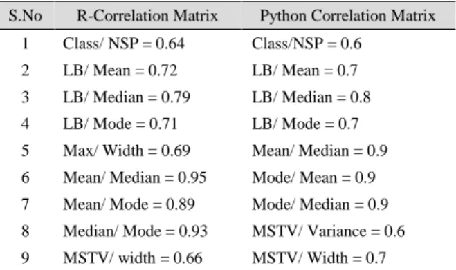
In order to improve the model accuracy, a subset of relevant features can be useful for better model building. In this study, a highly correlated attributes were selected based on the correlation analysis. The correlation plot in R (Figure 3a) and Python (Figure 3b) of 0.6–1.0 was taken as positive strong correlation [31]. The topology of the highly correlated features was found to be similar both in R and Python, except for MSTV/ Variance = 0.6 (in Python, Table 4).
Table 4 Correlation of Features
S.No R-Correlation Matrix Python Correlation Matrix 1 Class/ NSP = 0.64 Class/NSP = 0.6
2 LB/ Mean = 0.72 LB/ Mean = 0.7 3 LB/ Median = 0.79 LB/ Median = 0.8 4 LB/ Mode = 0.71 LB/ Mode = 0.7 5 Max/ Width = 0.69 Mean/ Median = 0.9 6 Mean/ Median = 0.95 Mode/ Mean = 0.9 7 Mean/ Mode = 0.89 Mode/ Median = 0.9 8 Median/ Mode = 0.93 MSTV/ Variance = 0.6 9 MSTV/ width = 0.66 MSTV/ Width = 0.7
10 Nmax/ Width = 0.75 Width / Variance = 0.6 11 Width / Variance = 0.62 Width/ Max = 0.7
12 Nil Width/ Nmax = 0.7
(a)
(b)
Figure 3: Correlation plot with complete features using (a) R, and (b) Python
It is important to remove one feature among a set of strongly correlated features as they show an effect on model performance. The order of topology with minor differences in the ranking order has been noticed in the four methods (RFE-RF, RFE-SVMpoly in R and RFE-LR, SelectKBest/f_classif in Python, refer to Table 5). Thus, the feature(s) are preferred over other features as the relevant ones based on the ranking order shown by the feature selection methods. In this study, the nine correlated attributes are class, mean, median, mode,
91.48 91.1 88.48 83.18 86.28 83 75 80 85 90 95
Accuracy Precision Recall
width, max, Nmax, MSTV and variance. Thus remaining 14 attributes was taken into consideration for model building.
Table 5
The Best Selected Features from R and Python Packages
R Python
RFE- RF RIF-SVM poly RFE – LR SelectKBest/f_classif CLASS ASTV ALTV Mean AC MSTV Mode Median LB MLTV Variance DP Width Max UC DL Min Nmax FM Tendency Nzeros DS CLASS 0.462 ASTV 0.299 DP 0.228 AC 0.217 MLTV 0.186 Mode 0.125 Mean 0.123 ALTV 0.104 Median 0.103 Variance 0.067 DL 0.037 Tendency 0.030 DS 0.011 UC 0.009 LB 0.008 Max 0.004 FM 0.001 Nmax 0.0007 Width 0.0005 Nzeros 0.0002 NSP MSTV DP AC CLASS DL Nmax Mean LB Nzeros UC DS Tendency MLTV Median Mode ALTV ASTV Max Variance FM Width Min CLASS 623.89 Mean 251.94 Median 224.35 ASTV 214.25 Mode 210.52 DP 191.69 AC 162.63 LB 123.77 ALTV 90.20 MSTV 88.65 Variance 86.95 MLTV 79.15 DL 75.51 Min 64.84 Width 40.20 Tendency 38.09 UC 25.41 Nmax 11.91 DS 8.15 Max 2.14 Nzeros 2.08 FM 1.87
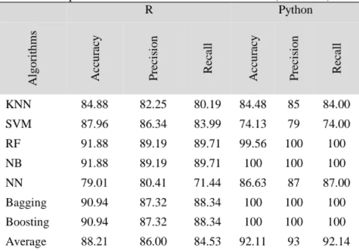
C. Performance on Feature Selected Attributes
The selected 14 attributes were taken into consideration to build a model. The highest accuracy in ‘R’ with the similar performance of the classifiers has been observed in the random forest and naïve Bayes followed by bagging and boosting respectively. Whereas in ‘Python’, the highest accuracy has been observed in bagging, boosting, naïve Bayes and random forest (100% and 99.56%) respectively. The same goes with respect to the precision and recall (Table 6). In comparison to both R and Python, the ‘Python’ shows the highest average accuracies (92.11%) and the same goes with respect to precision and recall (93% and 92.14%) (Table 6 and Figure 4). This indicates that the Python tool performed better than ‘R’ (refer to Table 3 and Figure 2).
Table 6
The Performance Comparisons of R and Python Machine Learning Techniques in Balanced Dataset with 14 Features (Attributes)
R Python A lg o ri th ms A cc u ra cy P re ci si o n R ec al l A cc u ra cy P re ci si o n R ec al l KNN 84.88 82.25 80.19 84.48 85 84.00 SVM 87.96 86.34 83.99 74.13 79 74.00 RF 91.88 89.19 89.71 99.56 100 100 NB 91.88 89.19 89.71 100 100 100 NN 79.01 80.41 71.44 86.63 87 87.00 Bagging 90.94 87.32 88.34 100 100 100 Boosting 90.94 87.32 88.34 100 100 100 Average 88.21 86.00 84.53 92.11 93 92.14
Figure 4: Average accuracy, precision, and recall of R and Python (14 attributes)
D. Performance of the Correlated Attributes
From the above results, it is known that R performs better with the whole dataset (23 attributes), whereas Python performs better with the feature selected attributes (14 attributes), the results are in contrast with the machine learning techniques, tools and parameters setting (i.e., R and Python). We therefore, looked into the classification performance of ML techniques with respect to nine correlated attributes to know how far these features contribute to the performance being provided the same parameters as explained in data analysis for complete and selected features. In comparison to both R and Python, the ‘R’ shows the highest average accuracies (95.07%) and the same goes with respect to precision and recall (93.99% and 93.63%; Table 7 and Figure 5).
Table 7
The Performance Comparisons of R and Python Machine Learning Techniques in Balanced Dataset with 9 Features (Attributes)
R Python A lg o ri th ms A cc u ra cy P re ci si o n R ec al l A cc u ra cy P re c is io n R ec al l KNN 94.48 92.88 92.83 78.01 78.00 78.00 SVM 88.09 88.34 83.91 65.51 74.00 66.00 RF 96.96 95.98 96.24 100 100 100 NB 96.96 95.98 96.24 100 100 100 NN 96.22 95.25 95.24 88.36 89.00 88.00 Bagging 96.39 94.76 95.48 100 100 100 Boosting 96.39 94.76 95.48 100 100 100 Average 95.07 93.99 93.63 90.26 91.57 90.28
Figure 5: Average accuracy, precision, and recall of R and Python (9 attributes)
VI. DISCUSSION
In this study, the classification and feature selection algorithms implemented in the CARET package of R tool and Scikit learn package of Python-tool have been used to evaluate “this study CTG dataset” with complete and reduced features. The classification accuracy with complete features
88.21 86 84.53 92.11 93 92.14 80 85 90 95
Accuracy Precision Recall
R Python 95.07 93.99 93.63 90.26 91.57 90.28 86 88 90 92 94 96
Accuracy Precision Recall
is shown by random forest, naïve Bayes and the highest average accuracy (R-ML techniques). The results are in accordance with the previous studies where classification accuracies have been studied with UCI repository CTG dataset [14, 16]. On the other hand, the 14 selected features with the highest accuracies and similar performance are shown by naïve Bayes, bagging, boosting and the average accuracy (Python-ML techniques). Despite of the different tools, it is found that 14 selected features show similar results with the 23 attributes datasets, indicating the selected features could be used for the prediction of CTG data [15], and shows the best performance with the previous studies where similar feature selections methods and classification models are used with the UCI repository CTG dataset [20, 22, 24]. It is also noticed that the increase in accuracy with respect to the 23 attributes could be due to the increase in classifier performance with the nine correlated features under the given parameters (R-ML techniques). However, this scenario is not observed in Python-ML techniques, indicating classification studies should be taken into account not just based on models and parameter settings, and it also shows the importance of the tools used.
VII. CONCLUSION
The present study shows the evaluation of the derived dataset. The complete and reduced features of the dataset show similar results when compared with the UCI repository CTG dataset. Despite the different tools used, this study shows good accuracies in random forest, naïve Bayes of complete and reduced features (R-ML techniques), whereas naive Bayes, bagging and boosting are found to be showing good accuracies in reduced features (Python-ML techniques) with an accuracy of 91.88%100%. The less variation of accuracy differences between complete and selected features (23 and 14) indicates the selected features can be useful for the prediction of derived CTG dataset. However, it is also shown that correlated features contribute to the increase of classification accuracy; thus, it is necessary to keep track of these reduced features while performing classification modeling in a way to know which features could be useful for better prediction of CTG data. Based on this study, it is known that the database, preprocessing, analytical techniques and tools with respect to the nature of dataset play a role for model classification accuracies.
REFERENCES
[1] M.L Huang, and Y.Y. Hsu “Fetal distress prediction using discriminant analysis, decision tree, and artificial neural network,” J. Biomedical
Science and Engineering, vol. 5, pp. 526-533, 2012.
[2] O. Maimon, and L. Rokach, The Data mining and knowledge discovery
handbook, New York Springer, 2005.
[3] M. Romano, M. Bracale, M. Cesarelli, “Antepartum cardiotocography: A study of fetal reactivity in frequency domain”, Computers in Biology
and Medicine, vol.36, 619-633, 2006.
[4] J.T. Parer and E.G. Livingstone, “What is fetal distress”, Am J obstet
Gynecol, vol. 162, 1421-1425, 1990.
[5] M. Gupta, T. Nagar, and P. Gupta, “Role of cardiotocography to improve perinatal outcome in high risk pregnancy”, International
Journal of Contemporary Medical Research, vol. 4, 853-856, 2017.
[6] D. Gavrilis, G. Nikolakopoulos, and Georgoulas G, “A one-class approach to cardiotocogram assessment”. Conf Proc IEEE Eng Med
Biol Soc, pp. 518-521, 2015.
[7] D. Ayres-de-Campos, C. Costa-Santos, J. Bernardes, and S.M.V.S. Group, “Prediction of neonatal state by computer analysis of fetal heart rate tracings: the antepartum arm of the SisPorto® multicentre
validation study”, Eur. J. Obstet. Gynecol. Reprod. Biol, vol. 118, pp. 52-60, 2005.
[8] C. Sundar, M. Chitradevi, and G. Geetharamani, “Classification of cardiotocogram data using neural network based machine learning technique,” International Journal of Computer Applications, vol. 47, pp. 19-25, 2012.
[9] N. Jothi, N.A. Rashid, and W. Husain “Data mining in healthcare-A review”, Procedia Comput. Sci, vol. 72, pp. 306-313, 2015.
[10] H. Sahin, and A. Subasi, “Classification of the cardiotocogram data for anticipation of fetal risks using machine learning techniques,” Applied
Soft Computing, vol. 33, pp. 231-238. 2015.
[11] G. Georgoulas, C. Stylios, V. Chudáček, M. Macas, J. Bernardes, and L. Lhotska, “Classification of fetal heart rate signals based on features selected using the binary particle swarm optimization algorithm,”
World Congress on Medical Physics and Biomedical Engineering, pp.
1156-1159, 2006.
[12] N. Chamidah and I. Wasito, "Fetal state classification from cardiotocography based on feature extraction using hybrid K-Means and support vector machine,” International Conference on Advanced
Computer Science and Information Systems (ICACSIS), Depok, 2015,
pp. 37-41. 2015.
[13] D. Jagannathan “Cardiotocography - a comparative study between support vector machine and decision tree algorithms”. International Journal of Trend in Research and Development, vol 4, pp. 148-151, 2018.
[14] M. Arif “Classification of cardiotocograms using random forest classifier and selection of important features from cardiotocogram signal”. Biomaterials and Biomechanics in Bioengineering, vol. 2, pp.173-183, 2015.
[15] S. A. A. Shah, W. Aziz, M. Arif, and M.S.A Nadeem, “Decision trees based classification of cardiotocograms using bagging approach,” 13th International Conference on Frontiers of Information Technology
(FIT), Islamabad, pp.12-17, 2015.
[16] D. Bhatnagar, and P. Maheshwari, “Classification of cardiotocography data with WEKA,” International Journal of Computer Science and
Network, vol. 5, pp. 412-418, 2016.
[17] V. Subha, D. Murugan, J. Rani, and K. Rajalakshmi “Comparative analysis of classification techniques using cardiotocography dataset,”
International Journal of Research in Information Technology, vol. 1,
pp. 274-280, 2013.
[18] Z. Cömert, and A.F. Kocamaz, “Comparison of machine learning techniques for fetal heart rate classification,” Acta Physica Polonica A, vol. 132, pp. 451-454, 2017.
[19] H. Tang, T. Wang, M. Li, and X. Yang, “The design and implementation of cardiotocography signals classification algorithm based on neural network,” Computational and Mathematical Methods
in Medicine, Article ID 8568617, pp. 1-12, 2018.
[20] Y. Zhang, and Z. Zhao “Fetal state assessment based on cardiotocography parameters using PCA and AdaBoost,” 10th International Congress on Image and Signal Processing, BioMedical
Engineering and Informatics (CISP-BMEI), Shanghai, pp.1-6, 2016.
[21] E.M. Karabulut, T. Ibrikci, “Analysis of cardiotocogram data for fetal distress determination by decision tree based adaptive boosting approach”. Journal of Computer and Communications, vol. 2, pp. 32-37, 2014.
[22] S.A. Dongare, V.N Ande, and R.K. Tirandasu “A feature selection approach for enhancing the cardiotocography classification performance,” International Journal of Engineering and Techniques, vol. 4, pp. 222-226, 2018.
[23] M. E. B. Menai, F.J. Mohder, and F. Al-Mutairi “Influence of feature selection on naïve bayes classifier for recognizing patterns in cardiotocograms,” Journal of Medical and Bioengineering, vol. 2, pp. 66 -70, 2013.
[24] P. Fergus, A. Hussain, D. Al-Jumeily, D.S. Huang, and N. Bouguila, “Classification of caesarean section and normal vaginal deliveries using foetal heart rate signals and advanced machine learning algorithms”, Biomed Eng Online, vol.16, pp. 1-26, 2017.
[25] Y. Sun, A.K. Wong, and M.S. Kamel, “Classification of imbalanced data: a review,” International Journal of Pattern Recognition and Artificial Intelligence, vol 23, pp. 687-719, 2009.
[26] R.M.O Cruz, S. Robert, and G.D.C Cavalcanti, “On dynamic ensemble selection and data preprocessing for multi-class imbalance learning,”
Proceedings of the ICPRAI, pp. 189-194, 2018.
[27] S.P. Potharajua, M. Sreedevia, V.K. Andeb, and R.K. Tirandasub, “Data mining approach for accelerating the classification accuracy of cardiotocography,” Clinical Epidemiology and Global Health, doi.org/10.1016/j.cegh.2018.03.004, In Press, 2018.
[29] I.H. Witten, E. Frank, and M.A. Hall, “Data Mining: Practical Machine Learning Tools and Techniques,” (3rd Edsn). Morgan Kaufmann; New York, Sydney, 2011.
[30] T. Silwattananusarn, W. Kanarkard, and K. Tuamsuk, “Enhanced classification accuracy for cardiotocogram data with ensemble feature
selection and classifier Ensemble”. Journal of Computer and Communications, vol. 4, pp. 20-35, 2016.
[31] C. Ray, and A. Ray, “Intrapartum cardiotocography and its correlation with umbilical cord blood pH in term pregnancies: a prospective study.” International Journal of Reproduction, Contraception,