Implementation of a GNU Radio and Python
FMCW Radar Toolkit
Themba W. Mathumo
∗†, Theo G. Swart
∗and Richard W. Focke
†∗Depart. of Electrical and Electronic Engineering Science, University of Johannesburg, South Africa
†Defence, Peace, Safety and Security, Council for Scientific and Industrial Research, South Africa
[email protected], [email protected], [email protected]
Abstract—The use of GNU Radio in order to explore FMCW radar is growing rapidly, where it is used for radar signal pro-cessing. In this paper we implement FMCW surveillance radar for drone detection on SDR using GNU Radio and the USRP B210. The requirement was to design and implement an FMCW surveillance radar to detect a drone with a radar cross-section of 0.1 m2and a maximum range of 150 m for the purpose of point detection. The signal processing takes the beat frequency which has pulse compression gain and performs coherent integration. It windows and displays the results on a range Doppler map using two-dimensional fast Fourier transform. The pulse repetition frequency of the waveform is selected as 2200 Hz with a chirp bandwidth of 28 MHz, allowing for resolving a maximum velocity of 30 m/s unambiguously, which is the typical maximum speed of a small drone. Experiments were conducted using a human being and a car target as a drone was not available. The B210 induced a phase drift in the results which causes a Doppler shift. The phase drift was resolved by creating a phase equalization matrix, which was used to correct the phase drift in real-time. Verification of the designed radar system yielded a 63% probability of detection and probability of false alarm of1.7×10−6.
Index Terms—Doppler radar, frequency modulation, radar signal processing, software defined radar
I. INTRODUCTION
There is a growing demand for cheap portable radar sys-tems which are configurable and can be used for different applications. Typical examples are for medical imaging [1] and synthetic aperture radar (SAR) [2].
Software defined radio (SDR) is a radio transceiver in which most of the key parameters of radio operations, that are typically implemented in hardware, are implemented in software. SDR has allowed radar to be explored in software [3]. Radar is primarily used to measure range and radial velocity using transmission and reception of radio frequency (RF) and signal processing. GNU Radio is one of the platforms that is used for designing software defined radar together with the Universal Software Radio Peripheral (USRP) as front end. Ralston and Hargrave [3] introduce ground penetrating radar (GPR) and the concept of using SDR for radar ranging. The requirements for GPR radar are usually high bandwidth, timing accuracy and high transmit power. The prototype was built using GNU Radio and USRP2 since these are open source and generic.
Sundaresanet al. [4] discuss SDR radar as a potential tech-nology to be used for target detection and tracking. Prabaswara
et al. [5] discuss the use of SDR radar for weather surveillance
purposes. Both studies have a similar implementation: USRP N210 and GNU Radio are used in their conceptual designs using FMCW waveform.
Research and development on Reconfigurable Hardware Interface for Computation and Radio (RHINO) is being done at the University of Cape Town [6]. RHINO is an open source development consisting of hardware and software which is also designed for radar application. Such hardware opens the opportunity for the practical realization of radar.
The application area of drone detection is of interest as drones are gaining popularity in transportation and are also increasingly being used for criminal purposes, such as spying and transportation of drugs into prison [7]. Thus, it is of interest to determine whether SDR is capable of being used for radar surveillance applications, as it could lead to radar systems deployable against the increasingly prevalent drones.
II. FMCW WAVEFORMS
Frequency-modulated continuous-wave (FMCW) radar has been the center of interest when designing radar in GNU Radio because of its low power requirements and low cost [5]. An FMCW waveform, also known as a chirp, is modeled as [8]:
f(t) =fT +fdev
T t, (1)
wheref(t)is the transmitted waveform of a center transmit frequency fT plus the slope. The slope is the relationship between fdev and T, where fdev is the stop frequency of the
chirp in hertz. Fig. 1 shows the reflected signal from a moving target, where the signal shifts up or down because of the Doppler effect. The problem is that the beat frequency consists of the Doppler and/or range component, and it is impossible to determine them using only one beat frequency.
A. Two-dimensional Signal Processing for FMCW Radar
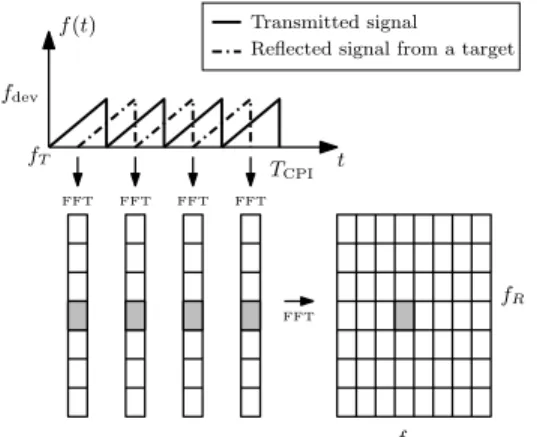
Since it is not possible to determine both range and velocity using a single up/down chirp, and since the triangular chirp does not work for multiple targets, the double fast Fourier transform (FFT) technique for FMCW signal processing is used for multiple targets, as shown in Fig. 2.
The chirp sequence is multiple pulses within a coherent processing interval (CPI), and TCPI is the dwell time at
which a number of pulses are transmitted and received. The transmitted signal is mixed with the Doppler-shifted and time-delayed reflected signal. The M pulses are arranged in a
f(t) fdev τ t TCPI fB fT Transmitted signal Reflected signal from moving target
Fig. 1. Up chirp transmitted waveform with time-delayed reflected waveform from a stationary target [9].
FFT FFT FFT FFT FFT fR fD f(t) t fT TCPI fdev Transmitted signal Reflected signal from a target
Fig. 2. Chirp processing by the method of pulse Doppler processing.
two-dimensional matrix in which range and Doppler FFT processing is performed in order to obtain a range Doppler matrix. Then the double FFT can be performed on the range Doppler matrix in order to obtain the range and radial velocity of targets.
III. SYSTEMDESIGN
The user requirement is to design and implement an FMCW ground-based surveillance radar. It should be able to detect small drones for the purpose of point defence, which is a low-range application, and have the following properties:
• A range coverage of up to 150 m—the maximum range allows time for detection and decision making after the target has been identified.
• Probability of detection of 80% is required for a 0.1 m2 target, with probability of false alarm of 10−6, meaning
1 false alarm per 1 million observations.
• The sampling rate that we could achieve using the B210 is 28 MHz, which results in the range resolution to be 5.35 m, and not 0.1 m as expected using the range resolution equation [10].
• A desired azimuth coverage of 45◦. The advantage of using a directional antenna is that the antenna can achieve higher gain, the narrower the antenna the higher the gain. A drone is relatively small, thus the 45◦azimuth coverage is enough for the radar to cover multiple drones in the direction that the radar is facing.
The performance of the low-cost USRP B210 transceiver is investigated for its performance for radar use in the C band. At the time of these investigations there was no previous radar work done using the B210.
A. Radar Waveform Design
The radar is designed based on user requirements which are then interpreted to be the design parameters using signal design rules [10]. The given user parameters are that the surveillance radar should be able to detect a drone as far as away as 150 m. The parameters are given in Table I. The design parameters were calculated using the above-mentioned signal design rules. The user parameters were adjusted depend-ing on the constraints imposed by the B210 and the result of waveform design. Instead of having range resolution of 0.1 m, the achieved range resolution is 5.35 m because of the maximum bandwidth achieved by the B210; the velocity resolution that was expected by the user is 1 m/s but only 1.2 m/s was achieved based on the chosen pulse repetition frequency (PRF).
B. Radar Model
Table II gives the specifications of the USRP B210 and the antenna available that can be used for the experiments. Only the important parameters which are used to determine the radar performance are listed.
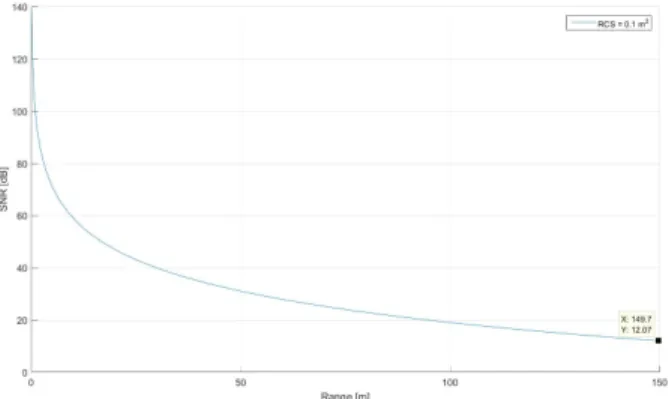
The radar characteristics are used to predict the radar performance by evaluating the SNR vs. range, as shown in Fig. 3. The SNR vs. range will be improved in order to meet the radar performance requirements.
The signal return of interest is buried under the noise floor since the SNR is negative. This means that during detection we will not be able to detect the targets.
The receiver operating characteristic (ROC) curve in Fig. 4 shows that in order to meet the user’s performance requirement the SNR has to be 12 dB. Various techniques such as intro-ducing amplifiers, the use of coherent integration and Doppler
TABLE I
THE USER PARAMETERS AND THE CALCULATED DESIGN PARAMETERS User
Value Design Value
Parameter Parameter
Center
5.5 GHz PRF 2200
frequency
Range Required: 150 m Number of pulses 50 Range Required: 0.1 m, Range of samples 227 resolution achievable: 5.35 m. Velocity 30 m/s Bandwidth 28 MHz Velocity Required: 1 m/s, CPI=#PRFpulses 22.73 m/s resolution achievable: 1.2 m/s. TABLE II
SPECIFICATIONS OF EQUIPMENT USED Parameter description Value
C-band 5.5 GHz Maximum transmit power 6.6 dBm Bandwidth 28 MHz Noise figure 3.8 dB
Fig. 3. SNR vs. range
Fig. 4. ROC curve for various SNR values. The SNR of the detector performance requirement is 12 dB.
processing gain will be employed to improve the current SNR to equal the performance requirement.
1) Effect of Low-noise Amplifier (LNA): The HMC460
LNA is introduced to improve the noise figure of the system, thereby improving the SNR. The LNA has a noise figure of 2.5 dB and a gain of 14 dB. The effective noise figure is determined by cascading the noise factor of the receive chain using Frii’s equation [9]:
N F(dB) = 10 log F1+ F2−1 G1 , (2)
whereF1 is the noise factor of the LNA, G1 the gain of the
LNA and F2 is the noise factor of the USRP B210.
2) Effect of Power Amplifier: The TWAL 0412-20 amplifier
was available, which is a 20 W amplifier with 43 dBm of power. The output power of the radar system is improved by 36 dB from the initial output power of 7 dBm.
3) Signal Processing Gain: The application of coherent
integration can help to improve the SNR, since multiple pulses will be transmitted. The returned pulses np can be integrated coherently by adding the I and Q data, which is equivalent to increasing the SNR by a gain of10 lognp.
Fig. 5 shows the improvement obtained in SNR vs. range when implementing these measures.
IV. IMPLEMENTATION
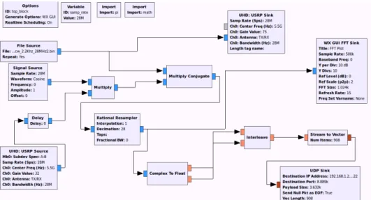
Fig. 6 is the design for the radar system. The SDR ap-proach allows less to be done in firmware but still builds on this technology by allowing the development to be done in software. The first step was to develop the independent GNU Radio block using C++ and Python that was responsible for generating the FMCW waveform using parameters of the
waveform design. Fig. 7 shows the flow graphs of the im-plemented GNU Radio block. The B210 handles the transmit and receive waveform and GNU Radio applies the process of dechirping. The controller is embedded in the FMCW transmitter block. The data from the FMCW transmitter is written in real time and is passed as meta data via JSON (Java Script Object Notation) so that further signal processing steps that require the data can proceed. Further processing was done in Python, and the data packets were sent using the user datagram protocol (UDP). Detection and windowing were performed and the results displayed in a two-dimensional range and Doppler plot.
The UDP has a 65535 byte maximum size that can be transferred as a payload, 8 bytes is the UDP header and 20 bytes is the IP header. It affects the design since there is a bottleneck for data that can be processed at the same time. The range samplesM was calculated to be 227 per pulse, when the pulse has PRF of 2200 Hz and the decimated sampling rate is 500 kHz. Since the data over UDP could not be complex, it was interleaved into float data which resulted in 454 samples being transferred over UDP. The waveform block was used to design the waveform, then the waveform was stored in a file using the GNU Radio file sink. The file source was used to
Fig. 5. SNR vs. range after implementing the LNA, power amplifier and pulse integration.
Fig. 7. GNU Radio implementation using the chirp signal which is displayed on the spectrum analyzer.
generate the waveform in real time and send the samples to the USRP.
The signal processing is done sequentially, as shown in Fig. 8. After receiving the meta data it is read from the JSON file that is shared over the network using Samba. The meta data sets the PRF, sampling rate, bandwidth, center frequency and the modulation waveform. The data is received from pulse to pulse and Hanning windowing is performed from pulse to pulse. According to the design, 50 pulses are received on which the two-dimensional FFT is performed. After the pulses have been coherently integrated, the result is displayed on an FFT plot. The pulses are arranged in a two-dimensional matrix and the windowing is done on the Doppler dimension together with the second FFT. The results are displayed on the two-dimensional Doppler range map.
V. RESULTS ANDDISCUSSION
In order to validate the transmit waveform according to the design parameters, we used a computer with GNU Radio installed. This computer was responsible for generating the waveform, and was connected to the USRP transmitting the signal, which was measured on the spectrum analyzer. The measured signal on the spectrum analyzer showed that the bandwidth of the signal was 28 MHz, shown in Fig. 9 by
∆Mkr, but the measured output power of the USRP was 1.39 dBm, and not the 6.6 dBm given in the specifications. The power of the signal is increased by the use of a power amplifier.
A human being and a car were used as targets in the experiments although the radar was designed to detect a drone. The experiments were done with reduced power: instead of the 43 dBm amplifier, a 13 dBm amplifier was used because of health implications and to account for using targets which have a bigger radar cross section (RCS) than a drone. Fig. 10 shows the setup and where the experiment was conducted.
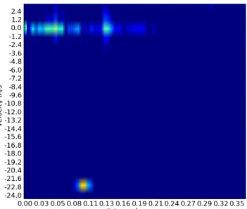
The target is approximately 60 m from the radar. The target and the clutter are not moving, so it is expected that they
Receive 2Msamples and createMcomplex pairs
Apply windowing on every pulse length
Get waveform parameters from meta
data CreateN×Mmatrix Windowing in Doppler dimension 2D FFT and FFT shift Store the complex data in a file Store the detections in a file
Plot 2D range and Doppler map
Perform CFAR detection on envelope
data Fig. 8. The signal processing algorithm.
Fig. 9. Measured signal on the spectrum analyzer.
should be at 0 m/s, but in Fig. 11 it is not centered at the 0 Hz Doppler bin due to the phase drift effect caused by the B210, the black line shows that the velocity is increasing with distance. The B210 contributes an unknown phase shift that varied with range on the range Doppler map.
To correct the phase drift, the phase correction algorithm shown in Fig. 12 was implemented in Python. The process was started by estimating the phase drift by calculating the slope of the phase drift. The Doppler shift is the rate of change of
Fig. 10. Setup used for the experiments.
Fig. 11. Range Doppler map without phase correction with clutter and stationary target that was placed at approximately 60 m.
phase [9], which is calculated using:
∇ϕ 2π =
2v
λP RF. (3)
The main aim of creating the equalization matrix was to create a negative slope with the same phase drift as the range Doppler matrix that had to be corrected. The phase drift was assumed to increase linearly, thus the equalization matrix was implemented in such a way that its phase drift increases linearly. The process of creating the 2D equalization matrix starts by creating a 1D array, with the data in increments of phase correction angle ϕ. The 1D array is transformed to 2D by incrementing the phase by the pulse number on the Doppler dimension—in the design 50 pulses were used for Doppler processing, thus the equalization matrix should be populated with 50 pulses so that the sizes are the same.
The data from the experiment was saved in a 2D FFT matrix, thus when it is read it undergoes inverse fast Fourier transform (IFFT) to get back to the time domain. Element-wise multiplication is performed between the experimental data and the equalization matrix, which has complex cosine and sine pairs. This will only cause phase change on the experimental data without affecting the amplitude, as can be shown using the Fourier transform pair [9]:
ej2πf0tx[n]←→X[f−f
0]. (4)
Estimate the needed phase drift (−ϕ)
Phase increment with pulseNin the Doppler dimension (2D matrix)
Element-wise multiplication with
cos(ϕ) and sin(ϕ)
Phase corrected range and Doppler map Populate 1D matrix with phase angleϕincrements
Perform 1D FFT and FFT shift in the Doppler dimension 1D IFFT on the Doppler dimension 1D FFT on the Doppler dimension and FFT shift 1D FFT in the
Doppler dimension Read 2D range Doppler
matrix from file
Fig. 12. Phase correction algorithm flow graph.
Fig. 13. Range Doppler map showing a car moving away from the radar. This is to test the radar for high speed.
After performing the element-wise multiplication in the time domain, the results are transformed back into the frequency domain and viewed on the range Doppler map.
In Fig. 13 we can see the car at the velocity of approxi-mately 20 m/s when the car was moving away from the radar. The phase drift has been corrected—there is no longer a slope or clutter, and the target has 0 Hz Doppler shift.
A. Probability of Detection Performance and Verification
In order to confirm the probability of detection a human was placed at a range of approximately 150 m, as it was specified from the user requirement for probability of detection of 80%. A number of trials should be repeated and saved to file to determine how many times the radar is able to detect the target; 1000 trials were performed. The human target was going back and forth in a circular motion within a distance of 5 m so that on the detector it will appear on the 28-th range bin. This will cause the RCS of the target to fluctuate since the range
resolution of the radar is 5.35 m and the target is moving in the range bin.
The target was detected 639 times out of the 1000 trials. The achieved Pd is 63.9%, but the expected probability of detection is 80%:
Pd=
Ndetections
Ntrials
. (5)
We use the Gaussian approximation to determine the con-fidence interval [11], where P is the mean of Pd, N is the number of trials and z is the critical value given for various values of probability: xL, xu=P±z r P(1−P) N , xL, xu= 0.639±0.013.
The reason why the detector could not perform optimally is that the strong signal return from the close-by objects may have masked the weak signal return from the target of interest as the RCS changes. From the design we could not meet the range resolution specification of 0.1 m for the RCS of 0.1 m2 target, the range resolution that was achieved is 5.35 m. This results in more clutter energy being integrated into a single cell along with the target, thus affecting the achieved SNR.
B. Probability of False Alarm Performance Verification
The other performance specification that needs to be met is the probability of false alarm. To do that the radar is directed in the vertical direction so that the radar only measures the leakage, thermal noise and opportunistic signals within the vicinity of the radar. A 100 trials of measurements are to be recorded, then we will use the constant false alarm rate (CFAR) detector to estimate the rate of false detections. The CFAR detector dynamically adjusts the threshold and, thus, it is not expected that noise will cause any false alarms. However, the system can generate spurious signal or receive opportunistic signals, thus once in a while a false target will be detected.
As a rule of thumb the value N should be at least N ≥ 10/Pf a, resulting in 100000000 trials [11]. Lower values of
N can still be used and relate it to time [9]:
Pf a =
TmF AR
M , (6)
whereF ARis the false alarm rate (i.e. how many false alarms occur in a second) and Tm is the time interval at which the number of resolution cells M are collected. Each trial consists of 226 samples of data, which represents a pulse at a PRF of 2200 Hz. The data capture was repeated for 100 trials. The calculated Pf a is 1.7×10⁻⁶, which is a good enough approximation for 1 false detection for 1 million radar observations.
VI. CONCLUSION
Drones are becoming popular for varying applications, but they are also being used for illegal activities such as spying and flying into restricted areas, thus a study of surveillance
radar using SDR (i.e. GNU Radio and B210) was done since it can be a portable and cost efficient solution.
A radar was designed and modeled using the given user requirements and performance specifications. The radar was expected to detect a drone up to 150 m away with 80% probability of detection and 10−6 probability of false alarm. The USRP B210 is part of the user requirements, and it had to be used as transceiver. It was studied in order to understand how it performs and what its limitations are. The waveform designed has PRF of 2200 Hz, at a center frequency of 5.5 GHz and bandwidth of 28 MHz; this results in resolution of 5.35 m, maximum unambiguous velocity of 30 m/s and velocity resolution of 1.2 m/s when 50 pulses are used for Doppler processing. The system was only capable of reaching 63.9% probability of detection and 1.7×10⁻⁶ probability of false alarm.
The bandwidth was still a limiting factor in terms of range resolution; however, reading the waveform from the file made it possible to increase the resolution. According to the spec-ifications of the B210, 56 MHz of instantaneous bandwidth can be achieved, but in the implementation only 28 MHz was achieved when both transmitter and receiver channels were used. The phase drift caused by the local oscillator of the B210 is one of the limiting factors in terms of getting an accurate Doppler shift. During the experiments a Doppler shift was induced, so a phase correction algorithm was implemented to solve the issue by creating an equalization matrix.
REFERENCES
[1] J. Marimuthu, K. S. Bialkowski and A. M. Abbosh, “Reconfigurable Software Defined Radar for medical imaging,” inAustralian Microwave Symp., Melbourne, Australia, Jun. 26–27, 2014, pp. 15–16.
[2] D. M. Chinnam, J. Madhusudhan, C. Nandhini, S. N. Prathyusha, S. Sowmiya, R. Ramanathan and K. P. Soman, “Implementation of a low cost synthetic aperture radar using software defined radio,” inInt. Conf. Computing Commun. Netw. Technol., Karur, India, Jul. 29–31, 2010, pp. 1–7.
[3] J. Ralston and C. Hargrave, “Software defined radar: An open source platform for prototype GPR development,” inInt. Conf. Ground Pene-trating Radar, Shanghai, China, Jun. 4–8, 2012, pp. 172–177. [4] S. Sundaresan, C. Anjana, T. Zacharia and R. Gandhiraj, “Real time
implementation of FMCW radar for target detection using GNU radio and USRP,” inProc. Int. Conf. Commun. Signal Proc., Melmaruvathur, India, Apr. 2–4, 2015, pp. 1530–1534.
[5] A. Prabaswara, A. Munir and A. B. Suksmono, “GNU Radio based software-defined FMCW radar for weather surveillance application,” in
Int. Conf. Telecommun. Syst. Services Applic., Bali, Indonesia, Oct. 20– 21, 2011, pp. 227–230.
[6] M. Inggs, G. Inggs, A. Langman and S. Scott, “Growing horns: Applying the Rhino software defined radio system to radar,” inIEEE Radar Conf., Kansas City, MO, May 23–27, 2011, pp. 951–955.
[7] (2016, June 26). Accurately detect and locate drones and their operators. Available: https://www.echoradarsystems.com/drone-detection-system/ [8] H. Rohling and M. Kronauge, “New radar waveform based on a chirp
sequence,”Int. Radar Conf., Lille, France, Oct. 13–17, 2014, pp. 1–4. [9] M. A. Richards, J. A. Scheer and W. A. Holm,Principles of Modern
Radar: Basic Principles, SciTech Publishing, 2010.
[10] D. E. Barrick, “FM/CW radar signals and digital processing,”NOAA Technical Report ERL 283-WPL 26, 1973.
[11] J. D. Echard, “Estimation of radar detection and false alarm probability,”
IEEE Trans. Aerosp. Electron. Syst., vol. 27, no. 2, pp. 255–260, Mar. 1991.