Imported Inputs and Productivity
∗
L´
aszl´
o Halpern
Institute of Economics, Hungarian Academy of Sciences and CEPR
Mikl´
os Koren
Central European University, IEHAS and CEPR
Adam Szeidl
Central European University, UC-Berkeley, NBER and CEPR
September 2011
Abstract
We estimate a model of importers in Hungarian micro data and conduct counter-factual policy analysis to investigate the effect of imports on productivity. We find that importing all foreign varieties would increase firm productivity by 12 percent, al-most two-fifths of which is due to imperfect substitution between foreign and domestic goods. The effectiveness of import use is higher for foreign firms and increases when a firm becomes foreign-owned. Our estimates imply that during 1993-2002 one-third of the productivity growth in Hungary was due to imported inputs. Simulations show that the productivity gain from a tariff cut is largest when the economy has many importers and many foreign firms, implying policy complementarities between tariff cuts, dismantling non-tariff barriers, and FDI liberalization.
∗E-mail addresses: [email protected], [email protected] and [email protected]. We
thank Istv´an Ily´es and P´eter T´oth for excellent research assistance, Pol Antr`as, P´eter Bencz´ur, Christian Broda, Jan De Loecker, Gita Gopinath, Penny Goldberg (the editor), Elhanan Helpman, Marc Melitz, Ariel Pakes, Roberto Rigobon, John Romalis, David Weinstein, two anonymous referees, and seminar participants for helpful comments. For financial support, Halpern and Koren thank the Global Development Network (Award RRC IV-061) and the Hungarian Scientific Research Fund (Award T048444) and Szeidl thanks the Alfred P. Sloan Foundation.
1
Introduction
Understanding the link between international trade and aggregate productivity is one of the major challenges in international economics. To learn more about this link at the microeco-nomic level, a recent literature explores the effect of imported inputs—which constitute the majority of world trade—on firm productivity. Studies show that improved access to foreign inputs has increased firm productivity in several countries, including Indonesia (Amiti and Konings 2007), Chile (Kasahara and Rodrigue 2008) and India (Topalova and Khandelwal 2011).1 The next step in this research agenda is to investigate the underlying mechanism through which imports increase productivity. As Hallak and Levinsohn (2008) emphasize, understanding which firms gain most, through what channel, and how the effect depends on the economic environment, are important for evaluating the welfare and redistributive implications of trade policies.
To explore these questions, in this paper we estimate a structural model of importer firms in Hungarian firm level data, and conduct counterfactual policy analysis in our estimated economy. Our starting point is a unique dataset that contains detailed information on im-ported goods for essentially all Hungarian manufacturing firms during 1992-2003. Motivated by stylized facts in these data, we formulate a model of firms who use differentiated inputs to produce a final good and must pay a fixed cost for each variety they choose to import. Imported inputs affect firm productivity through two distinct channels emphasized in the literature: they have a potentially higher price-adjusted quality as in quality-ladder models, and they imperfectly substitute domestic inputs as in product-variety models.2 Because of
these forces, firm productivity increases in the number of varieties imported. Our model also permits rich heterogeneity across products and firms.
In the first half of the paper we estimate this model in micro data. In doing so, we face the key empirical challenge that imports are chosen endogenously by the firm. We deal with this identification problem using a structural approach which exploits the product-level nature of the data. Our model implies a firm-level production function in which output depends on the usual factors of production as well as a new term related to the number of imported varieties. To estimate this production function, we follow Olley and Pakes (1996) in nonparametrically controlling for firm investment and other state variables, which pick up the unobserved component of productivity under standard assumptions. The import effect
1Results are conflicting for Brazil: Schor (2004) estimates a positive effect while Muendler (2004) finds
no effect of imported inputs on productivity.
2For quality-ladder models see Aghion and Howitt (1992) or Grossman and Helpman (1991). Variety
is then identified from residual variation in the number of imported varieties. Intuitively, we estimate the difference in output between two firms that have the same productivity, but differ in the number of varieties they choose to import—which, according to our model, happens because they face a different fixed cost of importing. We find substantial gains from imported inputs: in the baseline specification, increasing the fraction of tradeable goods imported by a firm from 0 to 100 percent would increase productivity by 12 percent. We then turn to decompose the import effect into differences in quality and imperfect substitution. We first note that for a given productivity gain from importing a particular good, the degree of substitution governs a firm’s expenditure share of foreign versus domestic purchases. For example, when foreign and domestic inputs are close to perfect substitutes, even if the productivity gain from imports is small the import share should be high.3 Based
on this idea, we then infer the relative magnitude of the two channels by comparing the expenditure share of imports for firms who differ in the number of imported varieties. While quality effects are important, we find that combining imperfectly substitutable foreign and domestic varieties is responsible for a substantial part—almost 40 percent—of the productiv-ity gain from imports. This finding parallels the evidence in Goldberg, Khandelwal, Pavcnik and Topalova (2009) that combining foreign and domestic varieties increased firms’ product scope in India; and also the theoretical arguments of Hirschman (1958), Kremer (1993) and Jones (2011) that complementarities, which amplify differences in input quality, may help explain large cross-country income differences.
We next explore whether the benefits from importing differ between foreign and domestic firms. Intuitively, because they have know-how about foreign markets and can access cheap suppliers abroad, foreign companies may gain more from spending on imports. This is an important possibility because foreign firms have played a very significant role in Hungary: during 1992-2003, their sales share in our data increased from 21 percent to 77 percent. When we re-estimate our model allowing for differences in the efficiency of import use by ownership status, we find that foreign companies benefit about 27 percent more than domestic ones from each dollar they spend on imports. To explore whether this large difference is directly caused by foreign ownership and not by selection, we use an event study in the subsample of initially domestic companies which were subsequently purchased by foreign investors. We find that the effectiveness of import use increases by 13.5 percent after a company changes owners (p-value of 9.9%), providing suggestive evidence—in a relatively small sample—that
3This link between import demand and the role of complementarities is also exploited by Feenstra (1994),
at least part of the advantage of foreign firms is caused by them being foreign-owned, and implying a complementarity between foreign presence and importing.
In the second half of the paper, we study the economic and policy implications of our estimates in two applications. We first quantify the contribution of imports to productivity growth in Hungary during 1993-2002. Our estimates imply a productivity gain of 15 percent in the Hungarian manufacturing sector, of which 6 percentage points, more than a third, can be attributed to import-related mechanisms. Approximately half of these import-related gains are due to the increased volume and number of imported inputs, while the other half is the result of increased foreign ownership in combination with foreign firms being better at using imports. These findings show both that imports contributed substantially to economic growth in Hungary, and the large aggregate effect of the complementarity between foreign presence and importing.
In our second application we use simulations in the estimated economy to explore the productivity implications of tariff policies. Intuitively, a tariff cut, by reducing the cost of and increasing access to foreign inputs, should raise both firm-level and aggregate productivity. Our main result is that the size of the aggregate productivity gain depends on two key features of the environment: (1) the initial import participation of producers; (2) the degree of foreign presence. Perhaps surprisingly, a higher initial import participation—more firms importing more kinds of products—implies larger gains from a tariff cut. This is because the set of inputs whose costs are affected is larger, and hence firms save more with the tariff cut. This logic also implies that the productivity effect of tariff cuts is convex: larger cuts have a more-than-proportional effect because they also increase the set of imported goods. In turn, foreign presence matters because, as we have shown, foreign-owned firms are better in using imports.
These patterns lead to complementarities between different liberalization policies. For example, our simulations show that tariff cuts increase productivity more when the fixed costs of importing—such as licensing or other non-tariff-barriers—are also reduced. Intu-itively, a lower fixed cost makes a larger set of goods available, expending the scope for cost-savings from the tariff cut. Because foreign firms are more effective in using imports, a similar complementarity exists between tariff cuts and FDI liberalization. While a careful analysis of other economies is beyond the scope of this paper, these complementarities seem broadly consistent with the liberalization experience in the early 1990s in India. Consistent with the first complementarity, tariff cuts in India, which were accompanied by dismantling substantial non-tariff barriers, lead to rapid growth in new imported varieties (Goldberg et al. 2009) and a large increase in firm productivity (Topalova and Khandelwal 2011). And
consistent with the second complementarity, these effects were stronger in industries with higher FDI liberalization (Topalova and Khandelwal 2011).
Our tariff experiment also highlights the differential policy implications of the quality and imperfect substitution mechanisms. We show that the demand for domestic inputs is more sensitive to tariffs when the benefit of imports comes from quality differences than when it comes from imperfect substitution. This is intuitive: when foreign goods are close to perfect substitutes, even a small price change can bring about large import substitution. Because our estimates assign a significant role to imperfect substitution, we obtain a relatively inelastic demand curve for domestic inputs. In addition, losses to domestic input suppliers caused by the tariff cut are partially offset by increased demand for their products due to higher firm productivity.4 One implication of these two forces is that redistributive losses due to import
substitution may not be very large in practice. A broader lesson from our counterfactual analysis is that identifying the mechanism through which imports affect productivity helps evaluate different trade policies.
Besides the papers cited above, we build on a growing empirical literature exploring firm behavior in international markets, reviewed in Bernard, Jensen, Redding and Schott (2007). Tybout (2003) summarizes earlier plant and firm level empirical work testing theories of international trade. Our structural approach parallels Das, Roberts and Tybout (2007) who study export subsidies, and Kasahara and Lapham (2008) who investigate the link between exports and imports, by estimating optimizing models. Our basic theoretical framework also builds on work by Ethier (1979) and Markusen (1989) who develop models connecting imported inputs and productivity.
The rest of this paper is organized as follows. Section 2 describes our data and documents stylized facts about importers in Hungary. Building on these facts, in Section 3 we develop a simple model of importer-producers. Section 4 describes the estimation procedure and results. In Section 5 we use these estimates to conduct counterfactual analysis. We discuss some caveats with our approach in the concluding Section 6.
4This logic parallels Grossman and Rossi-Hansberg (2008) who argue that offshoring can sometimes—
2
Data
2.1
Data and sample definition
Our panel of essentially all Hungarian manufacturing firms during 1992-2003 is created by merging trade and balance sheets data. Annual exports and imports for all firms, disaggre-gated by products at the 6-digit Harmonized System (HS) level (5,200 product categories), come from the Hungarian Customs Statistics. Because the 6-digit classification is noisy, we aggregate the data to the 4-digit level (1,300 categories), and we use the terms “product” and “good” to refer to a HS4 category in the rest of the paper.5 Firms’ balance sheets and profit and loss statements come from the Hungarian Tax Authority for 1992-1999, and from the Hungarian Statistics Office for 2000-2003. The data for 1992-1999 contain all firms which are required to file a balance sheet with the tax authority, i.e., all but the smallest companies—the main category of omitted firms are individual entrepreneurs without em-ployees. The data for 2000-2003 includes all firms with at least 20 employees and a random sample of firms with 5-20 employees. We thus lose some firms in 2000, which, however, constitute a relatively small share of output: during 1992-1999, firms with no more than 20 workers were responsible for less than 7.5 percent of total sales. We classify a firm to be in the manufacturing sector if it reports manufacturing as a primary activity for at least half of its lifetime in the data, and exclude all other firms. We merge the trade data and the balance sheet data using firms’ tax identifiers.
While our data contain product level information on imported input use, a limitation is that we do not have corresponding product-level data for domestic input purchases, because balance sheets only measure total spending on intermediate goods. We will rely on our struc-tural model and on input-output tables to work around this data issue. A second limitation is that we do not observe at the firm level import purchases from domestic wholesalers such as export-import companies. We can, however, measure the role of such indirect imports for the economy as a whole. We find that the total value of intermediate imports by wholesalers and retailers—as computed from our data—is about 2 percent of total intermediate input use by all firms in all sectors of the Hungarian economy. This result suggests that the role of intermediation is relatively small for intermediate goods, and due to lack of additional data we ignore it below.
Processing trade. An important source of measurement error in our data is that some firms engage in processing trade. In exchange for a fee, these firms import, process and
re-export intermediate goods which remain the property of a foreign party throughout. Be-cause the processing firm does not own, purchase or sell the underlying goods, processing trade is not recorded on the firm’s balance sheet, even though it appears in our trade data. This inconsistency creates measurement problems: in several observations, the value of im-ported intermediate inputs, as measured by customs,exceeds total spending on intermediate goods from the balance sheet. Similarly, exports measured in the customs data are often substantially higher than exports from the balance sheet.
To deal with this reporting discrepancy, we measure processing trade performed by a firm as the difference between customs exports and balance sheet exports (when positive). We classify a firm as “processer” in a given year if the ratio of processing trade to balance sheet sales exceeds 2.5 percent, which is approximately the median across observations where this ratio is positive. About 10 percent of our observations are classified as processers. To obtain measures which reflect the underlying economic activity rather than accounting rules, we then adjust, for all firms, sales and total intermediate spending from the balance sheet by adding our measure of processing trade.
Following these changes we create two data samples for our analysis. Ourmain sample is defined by excluding all firm-year observations in which the firm is classified as a processer. We also define a firm-level sample which is obtained by fully excluding firms which are pro-cessers for more than half of the years they are in our sample. The reason for the exclusions is that our adjustment for processing likely introduces considerable noise.6 Because it has
more observations, unless otherwise noted we will use the main sample in our analysis. The benefit of the firm-level sample is that, because it does not permit changes in the set of firms over time due to changes in processing activity, it better reflects aggregate trends in the data. After all exclusions, 130,027 observations remain in our main sample.
Input-output table. Besides the firm level data, we also make use of a sectoral input-output table at the 2-digit International Standard Industrial Classification (ISIC, revision 3) for the year 2000, which comes from the Hungarian Statistics Office.
2.2
Summary statistics and stylized facts
We document three basic facts about firms’ import behavior in the data, which will guide the specification of our formal model in Section 3.
6While we believe the exclusions are justified on prior grounds, keeping these firms in the sample and
Table 1: Descriptive statistics Full sample Non-importers Importers Employment 48.390 17.500 98.040 Sales (thousand USD) 2,908 392 6,952 Capital per worker (thousand USD) 12.990 10.700 16.660 Sales per worker (thousand USD) 49.410 35.340 72.030 Material share in output 0.662 0.636 0.705 Exporter indicator 0.351 0.149 0.675 Export share in output 0.108 0.047 0.205 Importer indicator 0.383
Import share in materials 0.105 0.274 Number of imported products
(HS4) 4.660 12.160
Foreign owned 0.157 0.071 0.296 State owned 0.027 0.020 0.037 Number of observations 130,027 80,162 49,865 Number of firms 27,074 21,361 13,556
Notes: Tables entries are means unless otherwise noted. Column 1 is based on the full sample defined in Section 2.1. Column 2 is computed for firm-years in which the firm does not import, and column 3 is computed for firm-years in which the firm does import. The number of firms in columns 2 and 3 add up to more than the total number of firms because of firms that switch importer status. USD values are in 1991 dollars.
Fact 1. There is substantial heterogeneity in the import patterns of firms. 61 percent of firms do not import at all; larger and foreign-owned companies are more likely to be importers.
This fact can be seen by comparing across columns in Table 1, which presents summary statistics for several key variables in our main sample separately for importing and non-importing firms. Importers employ about 6 times as many workers and sell about 18 times as much as non-importers. Using the classification that a firm is foreign-owned in a given year if foreigners have majority ownership, importers are also more frequently foreign owned and more likely to export.7 There is also substantial heterogeneity within importers in the number of products they import. Regressing the log number of imported products on log employment and foreign ownership shows that doubling firm size is associated with a 26 percent increase in the number of imported products, and, conditional on size, foreign firms import 144 percent more products than domestic firms. The patterns shown here are
7Firm level evidence from other countries shows similar patterns: for example, Bernard, Jensen and Schott
(2009) document that “globally engaged firms” in the U.S. are superior along a number of dimensions.
consistent with a model in which entry in import markets entails a fixed cost. Larger or more productive firms profit more from a given product and hence find it easier to overcome the fixed cost. Similarly, foreign firms may have lower fixed or variable costs of importing and hence purchase more foreign varieties.
Fact 2. Import spending is concentrated on a few core products; firms spend little on their remaining imports.
To document this fact, for each firm, we order imported products by the share of total import spending allocated to them. Using this ranking, among firms importing five or more products, the average spending share (out of total import spending) of the highest-ranked product is 54 percent. Thus, on average, firms spend more than half of their import budget on a single product. In contrast, the average spending share of the fifth-highest ranked product is only 3.5 percent. This substantial heterogeneity across goods may be important for evaluating the productivity gain from importing new products.
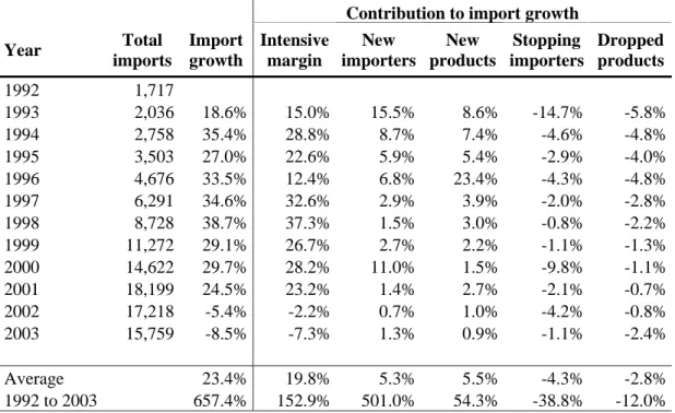
Fact 3. The extensive margin plays a large role in explaining both the aggregate trend and the firm level fluctuations in import growth.
Table 2, constructed from our firm-level sample, shows aggregate trends in firm imports over time. It is instructive to look at average annual growth as well as growth over the entire period of 1992-2003, reported in the last two rows. As column 3 shows, intermediate imports in the manufacturing sector grew by 23.4 percent per year on average, resulting in a total import growth of 657 percent between 1992 and 2003. On a year-to-year basis, almost 85 percent of import growth, 19.8 percent, is explained by the within-firm intensive margin, i.e., increased imports of goods that the firm was already importing in the previous year. Over the entire decade, however, the role of the extensive margin is much larger: imports of firms that did not import in 1992 and of products that were not imported in 1992 explain 84 percent of the growth in imports 1992-2003. The extensive margin also has a large yearly gross
volume: on average, new importers and newly imported products contribute 10.8 percent, while exit and the firm and the product level contribute -7.1 percent to import growth per year.8 These patterns call for an explicit model of the extensive margin of imports, and—
given the high frequency of exit at both the firm and product level—suggest that imports likely entail per-period fixed costs.
8Due to the change in sample definition in 2000, we lose some importing firms in that year (see Section
2.1). These firms are also classified as stopping importers in the table. Because we only lose firms with 20 or fewer employees, the vast majority of which do not import, their effect on the volume-weighted numbers in the table is likely to be small.
Table 2: Import dynamics
Contribution to import growth
Year Total imports Import growth Intensive margin New importers New products Stopping importers Dropped products 1992 1,717 1993 2,036 18.6% 15.0% 15.5% 8.6% -14.7% -5.8% 1994 2,758 35.4% 28.8% 8.7% 7.4% -4.6% -4.8% 1995 3,503 27.0% 22.6% 5.9% 5.4% -2.9% -4.0% 1996 4,676 33.5% 12.4% 6.8% 23.4% -4.3% -4.8% 1997 6,291 34.6% 32.6% 2.9% 3.9% -2.0% -2.8% 1998 8,728 38.7% 37.3% 1.5% 3.0% -0.8% -2.2% 1999 11,272 29.1% 26.7% 2.7% 2.2% -1.1% -1.3% 2000 14,622 29.7% 28.2% 11.0% 1.5% -9.8% -1.1% 2001 18,199 24.5% 23.2% 1.4% 2.7% -2.1% -0.7% 2002 17,218 -5.4% -2.2% 0.7% 1.0% -4.2% -0.8% 2003 15,759 -8.5% -7.3% 1.3% 0.9% -1.1% -2.4% Average 23.4% 19.8% 5.3% 5.5% -4.3% -2.8% 1992 to 2003 657.4% 152.9% 501.0% 54.3% -38.8% -12.0%
Notes: Total imports are in millions of 1991 USD. Columns 4-8 measure the percent increase in imports attributable to different mechanisms and sum to column 3 in each year. The intensive margin measures the contribution of (net) growth in imports of products that the firm also imported the previous period (which in all rows but the last is the previous year, and in the last row is 1992). New importers are firms that did not import in the previous period. New products are newly imported products of existing importers. Stopping importers and dropped products are defined analogously.
3
A Model of Firm Imports and Productivity
Motivated by the above stylized facts, we build a model of a firm which uses both domestic and imported intermediate goods for production. Section 4 will introduce the types of heterogeneity across firms that we allow in estimating this model.
3.1
Setup
Production technology. The output of the firm is given by the production function
Y = ΩKαLβ N Y i=1 Xγi i , (1)
where K and L denote capital and labor used in production, Xi denotes intermediate
weightγi measures the importance of goodifor production. Motivated by Fact 2, we allowγi
to be different for different goodsi.9 The total weight of all intermediate goods isγ =P
iγi.
Each intermediate good Xi is assembled from a combination of a foreign and a domestic
variety: Xi = h (BiXiF) θ−1 θ +X θ−1 θ iH iθ−θ1 , (2)
whereXiF and XiH are the quantity of foreign and domestic inputs, andθ is the elasticity of
substitution. The prices of the domestic and foreign varieties are denoted piH and piF, and
by adjusting units, we set piH = 1. The price-adjusted quality of the foreign input is then
Ai = Bi/piF. Intuitively, Ai measures the advantage of a dollar spent on a foreign relative
to a domestic variety.
To aid the estimation, we make several assumptions about intermediate inputs. In prac-tice some goods used for production are non-tradeable, and hence are not imported. To allow for non-tradeables in a simple way, we assume that they coincide with the set of services, and assign an infinitely high foreign price and hence Ai = 0 to these inputs. Doing this
will allow us to estimate the input share of non-tradeables from an input-output table. We also assume that the price-adjusted qualityAi of all tradeable goods used by the firm is the
same Ai = A > 0. This assumption greatly simplifies our analysis and still allows us to
estimate the average quality advantage of imports.10 Finally, we order indices so that in-puts 1,2..., Ng represent tradeable goods, while the remaining Ng+ 1, ..., N inputs represent
non-tradeable services. We also order tradeable goods by their production weight, so that
γ1 ≥γ2 ≥...≥γNg.
Motivated by stylized fact 3, we assume that the firm must pay a fixed cost F to access foreign markets, and that importing each variety has an additional fixed cost f which is constant across products within a firm. To make the model consistent with the high frequency of exit from import markets we assume that these costs are due every period.11
The firm sells its final good in a monopolistically competitive market, facing a firm-specific demand curve. For estimating the basic parameters, we require that the demand curve is sufficiently downward-sloping so that the solution to the firm’s profit-maximization problem exists.12 To obtain estimates of the fixed costs, and for the counterfactual analysis
9Hummels and Lugovskyy (2004) develop a related model where the marginal utility of additional varieties
declines.
10We do allow price-adjusted qualityAto vary across firms by industry, ownership status and over time
in the estimation.
11In the estimation we also explore the case whenF is a sunk cost.
12Denoting the (local) elasticity of demand by η, this is the case when α+β +γ < η/(η −1) holds
of Section 5.2, we impose a parametric isoelastic demand curve.
Discussion. Our production specification incorporates both the quality and variety gains from importing emphasized in the literature. Following Grossman and Helpman (1991), we interpret quality as the advantage in services provided by a good relative to its cost. The natural measure of the quality gain is therefore price-adjusted quality A, which can also be interpreted as the efficiency with which firms use imports, relative to domestic products, per dollar of spending. Imperfect substitution, i.e., the idea that combining foreign and domestic goods create gains that are greater than the sum of the parts, is measured by the elasticity of substitution θ. For θ finite, we always have a > logA: imperfect substitution amplifies the gain from a higher-quality foreign input. Our setup thus allows for flexibility in the degree of substitution as well as heterogeneity across inputs while maintaining the tractability of the Cobb-Douglas model. As we show below, this framework also gets around a data limitation by generating estimating equations for output and imports that involve only imported, but not domestic product level input purchases.
Because we are primarily concerned with the importing behavior of a firm at a point in time, the model introduced here is static. We make additional, standard, assumptions about firm dynamics in Section 4.1 to aid the estimation of this model in panel data.
3.2
Firm behavior
To characterize firm behavior, we first compute the cost-saving when the firm uses also imports for a particular composite good. Given the normalization that the domestic price of all inputs ispiH = 1, the effective price of a composite goodXi isPi = 1 if the firm only uses
the domestic inputXiH. If the foreign input is also used, the effective price can be found by
solving the cost-minimization problem associated with (2):
Pi =
piH+ (piF/Bi)1−θ
1/(1−θ)
=1 +Aθ−11/(1−θ) <1 (3) using the notation that Ai = Bi/piF and our assumption that Ai = A for all tradeable
imported inputs. The (log) percentage reduction in the cost of the composite good i when imports are used is therefore
a= ln
1 +Aθ−1
θ−1 . (4)
Parameter a measures the per-product import gain and hence is of central interest to us. Note that a incorporates the cost-savings created by both the quality and the imperfect-substitution channels: in particular, it is increasing in the price-adjusted quality A and decreasing in the degree of substitutionθ. Because of imperfect substitution, for finite θ the
firm uses both domestic and foreign inputs, so that the optimal expenditure share of the foreign good in the total spending for variety i, which can be computed as
s=Aθ−1/(1 +Aθ−1) (5) satisfies 0< s <1.
We next characterize the choice of which varieties to import. In this decision, the firm trades off the savings in marginal cost from using imports against the fixed costs of importing. Since the fixed costf and the per-product gain aare the same across products, a firm which imports n products will choose to import those with the highest γ weight, i.e., products
i = 1, ..., n. Let π(n, F, f) denote profits if the firm imports these n goods given cost realizations f and F.13 The optimal import decision of the firm is then
n= arg max
˜
n π(˜n, F, f). (6)
It is easy to see that n is weakly decreasing in f and F: firms with lower fixed costs import a greater number of varieties.
Once the firm sets n, the relative importance of imported inputs for production can be measured as the Cobb-Douglas share of composite goods which use imports relative to all intermediate inputs, which we denote
G(n) = Pn i=1γi PN i=1γi = Pn i=1γi γ . (7)
Since γ1 ≥ γ2, ... ≥ γg ≥ 0, the G(·) function is increasing and concave. Because the
denominator includes the weights of both goods and non-traded services, the maximum of
G(·), denoted ¯G=G(Ng), equals the share of tradable goods in all intermediate inputs.
We now useG(n) to connect the number of imported inputs to import demand and firm output. These two equations will form the basis for our empirical analysis. Denoting total expenditure on intermediate inputs byM =P
iPiXi and total expenditure on foreign inputs
byMF =PN
i=1piFXiF, the spending share on imports can be written as
MF
M =s
Pn i=1γi
γ =sG(n) (8)
wheres, defined in (5), is the optimal expenditure share of imports within a composite good
i. This equation links the import share to the number of imported varieties n. Intuitively,
13For notational simplicity we suppress the dependence ofπ on other firm level variables such askor ω.
The profit function can be calculated using the demand curve for the firm’s product, and we compute it explicitly in Appendix A for isoelastic demand.
firms that import a greater number of products n have a larger share of foreign goods in total intermediate spending. This effect is captured by G(n) because the Cobb-Douglas production function implies that the input share of each imported variety i equals sγi/γ.
For an optimizing firm, the following expression—proved in Appendix A—expresses total output with the number of imported varieties:
y =αk+βl+γm+aγG(n) +ω (9) where the lowercase variables y, k, l, m and ω denote logs. This equation has the form of a standard production function: the first three terms on the right-hand side measure the contribution of capital, labor and intermediate inputs to total output, while the final term is the Hicks-neutral productivity shifter ω. The novelty lies in the fourth term, which represents the contribution of imports. The intuition for this term is straightforward: a firm which chooses to import n varieties will have a percentage cost reduction of a on the associated composite inputs, the total weight of which isPn
i=1γi. This cost reduction maps
into a corresponding increase in output for a given total spending on intermediate inputs. A natural interpretation of equation (9) is that a firm’s total factor productivity is given by φ =aγG(n) +ω, i.e., the sum of the productivity gains from importing and a “residual productivity” term. This interpretation is correct in the sense that variation in φ measures differences in output for the same amount of resources employed in the production process; but it ignores the fact that importing also entails fixed costs which require resources. Thusφ
is an (approximately) correct measure of productivity holding fixed all resources only when the fixed costs are small relative to the overall productivity gain, which—because importing reducesmarginal costs but requires the payment offixed costs—is more likely to be the case for larger firms who import multiple different products.14 In the empirical analysis, we will compute an adjusted measure of productivity which also reflects the fixed costs of importing, and show that—because the bulk of production and importing is performed by mid-sized and large importers—the two measures generate essentially identical aggregate predictions. Hence in practice little is lost by treating φ as a measure of productivity, which is what we do below.
14More precisely, for the last product the firm chooses to import, the fixed cost should be approximately
the same as the savings induced by importing that product. For every other—inframarginal—product that the firm chooses to import, the fixed cost of importing is strictly lower than the cost-saving from lower marginal costs, and this difference is increasing in firm size because larger firms gain more from a given reduction in marginal cost.
4
Estimation and Results
We now turn to estimating the model in firm level data. Section 4.1 develops our empirical strategy and Section 4.2 presents the results.
4.1
Empirical strategy
Assumptions about firms and products. Our theoretical model is static and applies to a single firm. We now state assumptions about heterogeneity and dynamics which allow us to estimate this model in panel data.
Our empirical strategy assumes that firms can be partitioned into different groups—for example by industry or ownership status—such that certain model parameters are identical within a group, but can potentially differ between groups. The basic parameters α, β,γi, A
and θ are always held constant within a group, and we also make—standard—homogeneity assumptions about dynamics to ensure that the Olley-Pakes procedure yields consistent estimates within each group. Specifically, we write ωjt = ωobsjt +εjt for a firm j in period
t, where ωobs
jt is observable to the firm at the beginning of period t and εjt is a mean-zero
innovation, independent of other firm variables and identically distributed across firms in a group and over time. We assume that investment Ijt, which is set before εjt is realized, can
be written as Ijt =ξ(ωjtobs, zjt) where zjt is a vector of observable firm state variables which
always includes capitalkjt and calendar timet, and theξ function is the same across firms in
a group and is strictly increasing in its first argument. In addition, ωobs follows a first-order
Markov process with the same dynamics across firms in a group. These assumptions are common in the productivity literature. We also assume that the fixed costs Fjt and fjt are
drawn after the investment decision is made, independently across firms and over time, from a distribution that may depend on zjt and ωjtobs.
This framework allows for considerable heterogeneity within a group: firms can differ in their productivity, factor use, foreign and domestic intermediate input use, and also in their realized fixed costs. We also permit heterogeneity across products through theγiparameters.
The requirement that the γi—essentially, the G(·) function— are the same within a group
means that additional varieties decline in importance identically across companies, so that all firms in a group have the same production structure. Importantly, it does not mean that firms use the same goods in production, or that goods have the same production weight. For example, γ1, the share of the most important input, is the same for all firms; but this share
can be different from γ2, and also, the identity of the most important good can vary across
Estimating equations. We now use our assumptions to convert the production function (9) and the import demand equation (8) into estimable forms by substituting out G(n) and the productivity term ωobs. Because the shape of G(·) is unknown, we approximate it with an exponential function G(n) = ¯G[1−exp(−λn)] whose parameters ¯G < 1 and λ > 0 we estimate.15 To control for the productivity shifter ωobs, we follow Olley and Pakes (1996)
and invert the monotonically increasing investment function ξ to get
ωjtobs =h(Ijt, zjt)
with an unknown h “control” function, which is the same across all firms in a group.16 Substituting the expressions for G(·) and ωobs into (9) yields our first estimating equation
yjt =α·kjt+β·ljt+γ·mjt+δ·[1−exp(−λnjt)] +h(Ijt, kjt) +εjt, (10)
where δ = aγG¯, and given our assumptions, εjt is independent of all variables on the right
hand side.
Our second estimating equation substitutes the functional form for G(n) into import demand (8):
MF jt
Mjt
=s·G¯·[1−exp(−λnjt)] +ujt. (11)
Because the model implies this relationship exactly, without an error term, we assume that
ujt is classical measurement error orthogonal to the decision to enter import markets and
hence the number of imported inputs n.
Estimation. We now outline our empirical strategy and then explain the logic of identi-fication. Technical details are relegated to Appendix B. Estimation proceeds in two steps. First we estimate (10) and (11) jointly using nonlinear least squares, which, given our struc-tural assumptions, can also be thought of as a generalized method of moments estimation. To do this we nonparametrically estimate the unknown control function h(·) separately for each year as a third-order polynomial of z and investment, in which we also include a full set of 22 2-digit ISIC industry indicators.17 Given the identifying assumptions that ε and u
15In contrast to our assumptions about G(n), this functional form, which asymptotes to ¯G as n grows
without bound, has no maximum. Our implicit assumption, which is supported by our estimates, is thatNg is large enough that the difference between ¯GandG(Ng) is negligible. We obtained similar empirical results when we experimented with other functional forms forG(n) including splines.
16Becausez always includes calendar time, in effect we have a separatehfunction by year.
17 In our main specifications we do not include nonlinear functions of the industry indicators because, in
combination with the 12 year indicators, they would in effect create 264 groups—many of them small—for which a separate control function needs to be estimated, reducing power. Instead, below we report separate
are orthogonal to the right hand side variables, we obtain consistent estimates for β, γ, λ,
δ and s. We then compute aG¯ =δ/γ. To separately identify a and ¯G, we note that 1−G¯
should equal the expenditure share of services in total spending on intermediates, which we compute directly from a manufacturing input-output table.18 The second step is to estimate
the coefficients of state variables z such as capital, which we do the same way as Olley and Pakes.
Identification. The difficulty in estimating the production function (9) predicted by the model is that ω is potentially correlated with all variables on the right hand side, including
G(n). For example, more productive firms tend to import more kinds of products. By estimating (10) instead of (9), we substitute out productivity using structural assumptions in the spirit of Olley and Pakes. The identification of the import demand equation also follows from structural assumptions, which restrict the functional form on the right-hand side of (11). To see how natural threats to identification are resolved, consider the concern that more productive firms both spend more on imports and import a greater number of varieties, which could introduce spurious correlation between the left hand side and G(n) in (11). Importantly, our estimation is immune to this concern: productivity, which is explicitly incorporated in the model, cancels out of (11) because the left hand side is the share of imports in intermediate spending. While more productive firms do import more, they also spend more on intermediate goods, and given the homogenous production function, TFP drops out when we compute the ratio of these quantities. In fact, our structural assumptions yield a version of (11) which holdsexactly, with no error term—this is why, given our model,
u should be interpreted as classical measurement error.
It is useful to understand the variation which identifies our key parameters. Since we jointly estimate (10) and (11), the form of G(n) is determined as the shape traced out by the import share and by output when n varies, controlling for firm productivity. Once we have this shape, a and s are estimated from the coefficients ofG(n), and are thus identified from variation in n given controls. In effect, we are comparing the output of two equally productive firms who import a different number of varieties. In the model, such variation in n comes from the fixed cost f, which affects the optimal number of imported inputs. This step requires that the distributions of f and F have enough variation so that n is not spanned by our set of controls, which clearly holds in the data.
estimates for several large industries, in which all parameters, including the control function, can differ across industries.
As with all structural estimation, the validity of our identification is guaranteed only if the model is correctly specified. One important possible misspecification is that firms might differ in their efficiency of import useA. Such variation can generate heterogeneity insanda, which in turn can create correlation betweenuand G(n). We incorporate such heterogeneity in our empirical strategy by allowing different groups of firms to have a different A.
Recovering deep parameters. Onceaandsare estimated, we recover the deep parameters
A and θ which govern the strength of the quality and imperfect substitution channels. The basic idea is that a high a combined with a low s shows the importance of imperfect sub-stitution: even though imports are attractive (higha), the firm still uses a substantial share of domestic inputs (low s), indicating that mixing the two inputs is essential. Formally, we solve for A and θ from the following equations implied by the model:
−ln(1−s) = a·(θ−1), (12) lnA=a 1− ln s ln(1− s) . (13)
The first equation states that import demand s is positively related to both the gains from importing a and the degree of substitution θ−1. Intuitively, a given gain from imports a
maps into higher import demand when the elasticity is larger because importers are more willing to switch to foreign goods when they are good substitutes.19 Because we have both s
and a, this equation can be used to compute θ. The second equation (13) can then be used to back out the quality effectA. Here the intuition is that the difference between the quality effect lnA and the total gain from imports a is a reflection of imperfect substitution, which in turn is related to the import shares by the first equation.20
Consistency and standard errors. Our approach can be viewed as a GMM estimation and hence yields consistent estimates under our identifying assumptions. We obtain standard errors for all estimates from a bootstrap described in Appendix B.
Fixed costs. Finally we obtain measures, using some additional assumptions, for the fixed costs of importing. The idea is to invert equation (6), which expresses the optimal number of imported varieties n as a function off and F. Implementing this idea raises two conceptual issues. First, a firm’s choice of n depends not just on the import costs but also on the demand curve it faces. To make inference possible, we therefore assume that each
19This intuition is slightly imprecise because a reflects both the quality and the imperfect substitution
effects.
20Our approach here parallels Feenstra (1994) and Broda and Weinstein (2006). They express the
pro-ductivity (welfare) gain from variety asx1/(1−θ), wherex <1 is the new expenditure share of old varieties.
firm j faces an isoelastic demand curve Yjt = Otp
−η
jt , where we set η = 5, which is in the
range of estimates reported by Broda and Weinstein (2006), and the demand shifter Ot is
chosen so that we match total annual industry output in the data. Then equation (6) yields an explicit expression for n as a function of the fixed costs.
The second conceptual issue is that, becausenis a discrete variable, it does not pin down the exact values off and F. To deal with this problem, we first use (6) and the choice of n
to compute, for each importer, upper and lower bounds forf and an upper bound forF. We then make additional assumptions to parametrically estimate the probability distribution of the costs. We assume that logf is normally distributed with constant variance and a mean which depends linearly on zjt and ωobsjt , and we regress the log lower bound of f on these
variables to obtain the coefficients.21 We also assume that logF is normal with group-specific
mean and variance, and compute these parameters by matching the share of importers as well as the mean difference in log output between importers and non-importers in each group.22
Intuitively, higher fixed costs yield a lower share of importers, and higher dispersion in costs yields a smaller difference between the size of importers and non-importers.
4.2
Results
Table 3 summarizes our basic results. Because the dependent variable in the production function is log total sales, not value added, the coefficients of capital and labor are smaller than in the more common value-added specifications, while material costs have a large co-efficient. All columns include year and 2-digit ISIC industry fixed effects (of which there are 22) so that our parameters are identified from within year and within industry variation across firms.
Column 1 reports the results from our empirical procedure in a baseline specification.23
We estimate a highly significant per product import gain a of 0.174. This point estimate implies that the composite of the foreign and the domestic good is about exp(.174)−1 = 19 percent more efficient per dollar spent than the domestic good in itself. The share of
non-21Because the bounds we obtain are tight, estimating the regression using the upper bounds yields
essen-tially identical results.
22Armenter and Koren (2009) calibrate the fixed costs ofexporting the same way.
23Besides the year and industry effects, the control functionh(·) used to take out unobserved productivity
also contains third-order polynomials of investment and capital, estimated separately for each year and separately for domestic and foreign firms who might face different markets and hence a different investment decision. We also estimated specifications with separate control functions for the 22 2-digit industries (not reported) and obtained similar results.
Table 3: Baseline estimates Baseline Conditioning on exporter Conditioning on past imports Nonlinear least squares
Dep. Var.: log sales (1) (2) (3) (4)
0.029 0.029 0.031 0.023 Capital (α) (0.003) (0.003) (0.002) (0.002) 0.200 0.200 0.199 0.202 Labor (β) (0.003) (0.003) (0.003) (0.003) 0.788 0.784 0.782 0.791 Materials (γ) (0.003) (0.003) (0.003) (0.003) 0.174 0.123 0.057 0.146 Per-product import gain (a)
(0.046) (0.038) (0.03) (0.037) 0.666 0.674 0.674 0.670 Import share (s) (0.108) (0.108) (0.109) (0.104) 1.116 1.083 1.037 1.098 Efficiency of imports (A) (0.077) (0.054) (0.03) (0.060) 7.301 10.071 20.791 8.571 Elasticity of substitution (θ) [5.56;14.26] [7.11;22.61] [11.12;478.91] [6.55;14.33] 0.020 0.019 0.019 0.020 Curvature of G(n) (λ) (0.007) (0.007) (0.007) (0.007) 0.039 0.034 0.041 0.046 Foreign ownership (0.011) (0.011) (0.011) (0.008) 0.044 0.045 Exporter (0.004) (0.004) 0.012 Previous importer (0.005)
Industry indicators yes yes yes yes Year effects yes yes yes yes P-value of test for A=1 0.008 0.008 0.008 0.004
Olley-Pakes control function
Separately estimated: By year By year By year N/A Includes third-order polynomials of Investment, capital, foreign ownership As column 1 and exporter status As column 2 and past importer status N/A Observations 130,027 130,027 130,027 130,027
Notes: Bootstrapped standard errors clustered by firm are in parenthesis. For the elasticity of substitution (θ) we report a 95 percent confidence interval computed the same way in brackets. Columns 1-3 use the structural estimation procedure of Section 4.1 and column 4 is estimated from nonlinear least-squares. Industry indicators are 2-digit ISIC fixed effects. See Sections 4.1-4.2 and Appendix B for details.
service inputs among all intermediate inputs from the input-output table is ¯G= 0.825, and in column 1 the elasticity of output to intermediate inputs is estimated to be γ = 0.788. Combining these numbers, we predict that if a non-importer starts importing all tradeable varieties, it will experience an increase in log productivity ofaGγ¯ = 0.113, or a productivity gain of about 12 percent.
The table also reports our estimates of the structural parametersAandθ. In the baseline specification, the price-adjusted quality of foreign products relative to their domestic coun-terparts is A = 1.116, which is significantly greater than one. Imported inputs are thus 12 percent better than domestic per dollar of expenditure, and this difference in price-adjusted quality accounts for about 61 percent of the product import gain. The remaining 39 per-cent comes from imperfect substitution: we find that the elasticity of substitution between domestic and foreign goods is θ = 7.3. The basic empirical fact underlying the importance of imperfect substitution is that, in spite of the large gain from imports, the difference in the import share of firms who purchase more versus fewer foreign varieties is modest.
Column 2 re-estimates the model adding an indicator for export market participation in the production function. The reason is to distinguish the effect of imports from the “international engagement” of the firm, and to control for linkages between importing and exporting such as those emphasized by Kasahara and Lapham (2008). The control function in the Olley-Pakes procedure is now separately estimated by exporting status each year. The import estimates are slightly smaller but similar to the previous specification, suggesting that our procedure succeeds in isolating the impact of imports on productivity. Column 3 explores the possibility that entering import markets entails a sunk, rather than a fixed cost. When
F is sunk, the past importing status of the firm becomes a state variable, which should therefore be included both in the regression and in the control function. The estimates are now smaller, but the per product import gain is still significantly different from zero, and the results are qualitatively similar to our baseline. Taken together, these results show that imports have a significant productivity effect across specifications.
A robust finding in columns 1-3 of the Table is that imperfect substitution is responsible for 35−40 percent of the gains from importing. This result is consistent with the conclusions of Goldberg et al. (2009) who show, in micro data from India, that firms combine foreign and domestic varieties to increase their product scope: our results imply that combining these inputs also raises productivity. Our empirical finding that imperfect substitution amplifies the effect of higher quality inputs (i.e., that a >logA) parallels theoretical arguments that complementarities between inputs can generate large income differences across countries. As Jones (2011) explains: “high productivity in a firm requires a high level of performance along
a large number of dimensions. Textile producers require raw materials, knitting machines, a healthy and trained labor force, knowledge of how to produce, security, business licenses, transportation networks, electricity, etc. These inputs enter in a complementary fashion, in the sense that problems with any input can substantially reduce overall output. With-out electricity or production knowledge or raw materials or security or business licenses, production is likely to be severely curtailed.” Our findings provide support for the produc-tivity effect of this sort of interdependence in the context of combining foreign and domestic intermediate inputs.
Finally, column 4 reports the results from a specification which is the analogue of an OLS regression for our setting, in which equations (9) and (11) are jointly estimated with nonlinear least squares, but without using the Olley-Pakes procedure. Because this estimation does not fully control for firms’ endogenous choice of variable inputs, we expect the coefficients of labor and material to be upward biased due to the standard reverse causality problem which plagues OLS estimates of productivity. In the table these coefficients are almost identical across columns, suggesting that the reverse causality bias is modest in practice. This result is not uncommon in the literature; one possible explanation in our setting is that the year and industry fixed effects pick up a substantial part of the endogenous variation.
Foreign versus domestic firms. Foreign firms, defined as companies in which foreigners have majority ownership, have played a very significant role in the Hungarian economy. In particular, in our data their sales share increased from 21 to 77 percent during 1992-2003. Table 3, in which all specifications include an indicator for foreign ownership, shows that foreign companies are on average about 4 percent more productive than domestic ones, suggesting that their growing participation has had significant aggregate productivity effects in Hungary. This observation raises the question of whether foreign firms are more productive in part because the they use imports more efficiently. Indeed, these firms may find it easier to locate low-cost input suppliers abroad, may have more extensive know-how about foreign goods, and may face lower transactions costs.
To explore whether foreign-owned companies are more efficient in their import use, Table 4 reports estimates in which the price-adjusted quality of importsAis allowed to be different across firms with different ownership status. Maintaining the assumption that firms use the same technology, we restrict the elasticity of substitutionθto be the same for the two groups. The regression results in the first specification show a large and significant difference in the efficiency of import use: we estimate A = 1.18 for foreign owned firms, while A = 0.95, not significantly different from one, for domestic firms. The large difference in A maps into a correspondingly large difference in the log per-product import gain: we obtain a = 0.24
Table 4: The gains from importing for foreign and domestic firms
Cross-section Event study of change in ownership
(1) (2)
Dep. Var.: log sales Domestic Foreign Always domestic Before switching After switching Always foreign 0.03 0.027 Capital (α) (0.003) (0.002) 0.2 0.203 Labor (β) (0.003) (0.004) 0.788 0.784 Materials (γ) (0.003) (0.003) 0.116 0.241 0.126 0.125 0.191 0.288 Per-product import gain (a)
(0.024) (0.059) (0.035) (0.051) (0.059) (0.074) 0.435 0.695 0.444 0.442 0.59 0.739 Import share (s) (0.078) (0.089) (0.082) (0.088) (0.096) (0.092) 0.949 1.182 0.953 0.952 1.081 1.25 Efficiency of imports (A) (0.061) (0.095) (0.074) (0.084) (0.095) (0.12) 5.936 5.672 Elasticity of substitution (θ) [4.64;9.50] [4.27;8.94] 0.024 0.022 Curvature of G(n) (λ) (0.008) (0.008) 0.029 0.043 Foreign ownership (0.013) (0.012)
Industry indicators yes yes
Year effects yes yes
P-value of test for A=1 0.398 0.004 0.552 0.418 0.299 0.004 P-value of test that A =
previous column 0.004 0.972 0.099 0.016
Olley-Pakes control function
Estimated separately: By year By year Includes third-order
polynomials of
Investment, capital,
foreign ownership Investment, capital, foreign ownership
Observations 109,555 20,472 102,661 2,048 3,792 21,525
Notes: Bootstrapped standard errors clustered by firm are in parenthesis. For the elasticity of substitution (θ) we report a 95 percent confidence interval in brackets. Both specifications are estimated with the structural procedure of Section 4.1. A different efficiency of imports (A) is estimated in specification (1) for foreign and domestic firms; and in specification (2) for always foreign firms, firms switching from domestic to foreign before the change, the same firms after the change, and always foreign firms. Industry indicators are 2-digit ISIC fixed effects. See Sections 4.1-4.2 and Appendix B for details.
for foreign and a = 0.12 for domestic companies. These results also imply that domestic companies benefit from imports primarily through imperfect substitution.
From a policy perspective it is important to understand whether foreign firms’ greater ef-ficiency in import useAiscaused by them being foreign owned, or is due to other mechanisms such as selection, whereby foreign investors purchase firms which are better at using imports. To explore this question, we look for changes in the efficiency of import use in firms whose ownership status changes during our sample period. Intuitively, if foreign owners selectively purchase companies which are better at using imports, then the firm’s A should remain the same after the company changes ownership. In contrast, if foreign owners improve import use because of lower transactions costs or other mechanisms, then we expect A to increase after the company changes owners. Plausibly, this adjustment might occur slowly, over the course of multiple years, because the company needs to learn the more efficient way of using imports.
In the second specification of Table 4 we estimate a separate price-adjusted import quality
A for the following four groups of firms. (i) “Always domestic”: firms who are not foreign-owned at any point in the panel. (ii) “Before switching:” firms who are domestically foreign-owned in the current year but whose ownership status will change at a later date in the sample. (iii) “After switching:” the same firms in years following the change in ownership. (iv) “Always foreign” firms who are foreign-owned throughout our data. The table shows that switchers have A = 0.95 before the change—essentially identical to the estimate of A for always domestic companies—which increases to A= 1.08 once they become foreign-owned. The values of A before versus after the change in ownership are significantly different at a p-value of 9.9 percent. We also find that the efficiency of import use for always-foreign companies is A = 1.25. Keeping in mind that we do not expect immediate full adjustment under either hypothesis, and that the small sample size (there are 938 switcher firms in the data) does not allow for a more precise estimate, we interpret our results from ownership changes as strong suggestive evidence that foreign firms’ greater efficiency in import use is at least partly caused by them being foreign-owned. This evidence for causality suggests a potential policy complementarity between financial and trade liberalization, which we explore in greater detail in the next section.
Import effects by year and industry. To explore the robustness of our estimates and learn more about the impact of foreign goods on the Hungarian economy, we next explore how the gains from importing vary over time and across industries. Table 5 reports the efficiency of import use A estimated separately for foreign and domestic companies over three year intervals. Consistent with our earlier findings, throughout the sample period foreign firms
Table 5: The gains from importing over time
Dep. Var.: log sales 1992-94 1995-97 1998-00 2001-03
Efficiency of imports
Domestic firms 0.928 0.984 0.950 0.962 (0.071) (0.072) (0.078) (0.09) Foreign firms 1.052 1.320 1.198 1.151
(0.115) (0.164) (0.092) (0.107)
Other parameters (common across periods)
0.030 Capital (α) (0.002) 0.200 Labor (β) (0.003) 0.788 Materials (γ) (0.003) 5.758 Elasticity of substitution (θ) [4.242;8.511] 0.022 Curvature of G(n) (λ) (0.007) Foreign ownership 0.029 Industry indicators (0.015)
Year effects yes
P-value of domestic A=1 0.255 0.569 0.471 0.49 P-value of domestic
A=previous column 0.451 0.706 0.804 P-value of foreign A=1 0.510 0.020 0.020 0.020 P-value of foreign
A=previous column 0.059 0.392 0.725
Olley-Pakes control function Estimated separately: By year
Includes third-order
polynomials of Investment, capital, foreign ownership
Observations 130,027
Notes: Bootstrapped standard errors clustered by firm are in parenthesis. For the elasticity of substitution (θ) we report a 95 percent confidence interval in brackets. A different efficiency of imports (A) is estimated for foreign and domestic firms in each 3-year period using the structural procedure of Section 4.1. Industry indicators are 2-digit ISIC fixed effects. See Sections 4.1-4.2 and Appendix B for details.
Table 6: The gains from importing by industry
ISIC Sector Number of
observations Per-product import gain (a) Import share (s) Efficiency of imports (A) Elasticity of substitution (θ)
15 Food and beverages 19,441 1.304*** 0.935 3.568 3.100 18 Apparel 5,259 0.489** 0.938 1.613** 6.670 20 Wood products 8,061 0.228** 0.810 1.220 8.270 22 Printing and publishing 15,258 0.223*** 0.697 1.168*** 6.350 25 Rubber and plastics 7,534 0.194*** 0.724 1.156*** 7.650 26 Non-metallic minerals 5,252 0.05*** 0.424 0.973 12.070 28 Fabricated metal products 18,155 0.237*** 0.801 1.227** 7.790 29 Machinery 14,203 0.124*** 0.465 0.973 6.070 33 Instruments 5,339 0.28** 0.796 1.271* 6.660
Notes: Table reports industry estimates of our baseline specification for industries with more than 5,000 observations. Significance levels (* at 10 percent, ** at 5 percent, *** at 1 percent) for the tests a=0 and A=1 are obtained from a bootstrap clustered by firm. In each industry, the Olley-Pakes control function is estimated separately by year and includes third-order polynomials of investment, capital and foreign status. See Sections 4.1-4.2 and Appendix B for details.
are better in using imports. The table also shows a large increase in the efficiency of import use between the 1992-94 and the 1995-97 period. This finding is consistent with the rapid trade liberalization taking place in Hungary in the early 1990s, which reduced the effective price of imports, increasing price-adjusted qualityA. The 1992 Interim Agreement with the European Economic Community phased out most tariffs—the import-weighted tariff rate declined from 7.8 percent in 1992 to 3.2 percent in 1996—and Hungary joined the Central European Free Trade Agreement in 1992.
We also examine how the import effect varies by industry. Because different industries might face different production possibilities and a different market structure, we re-estimate our baseline specification separately for each of the 9 ISIC industries in which there are more than 5,000 firm-year observations. We allow for different capital, labor and material coefficients as well as a different G(n) and different Olley-Pakes proxy functions for each industry. Table 6 reports our estimates of the key model parameters by industry.24 Because
each industry has a smaller number of observations, the estimates are noisier, but the table confirms the main patterns identified earlier. Imports have a significantly positive produc-tivity effect in all 9 industries; and imperfect substitution is responsible for 42 percent of
24Significance levels are indicated by stars for the per-product import gain a and for the efficiency of
importsA.
these gains on average. The table also shows some interesting variation across industries. The largest per-product import gain—over 130 percent—is in food and beverages, while the smallest—about 5 percent—is in non-metallic minerals. Our estimates imply that the differ-ence between these two industries is due to the combination of the two productivity channels: imports are imperfectly substitutable and high-quality in the former industry, while they are close substitutes and relatively low quality in the latter. It seems also intuitively plausible that inputs in non-metallic minerals should be more substitutable then those in the food industry. The industry results also highlight how deep parameters are determined by our coefficient estimates. For example, both the wood products industry and printing and pub-lishing have a per-product import gain of about 22 percent; but because in wood products the import share estimate is larger, our model implies a higher elasticity of substitution. Intuitively, given the quality advantage of foreign goods, a higher import share must come from greater substitutability.
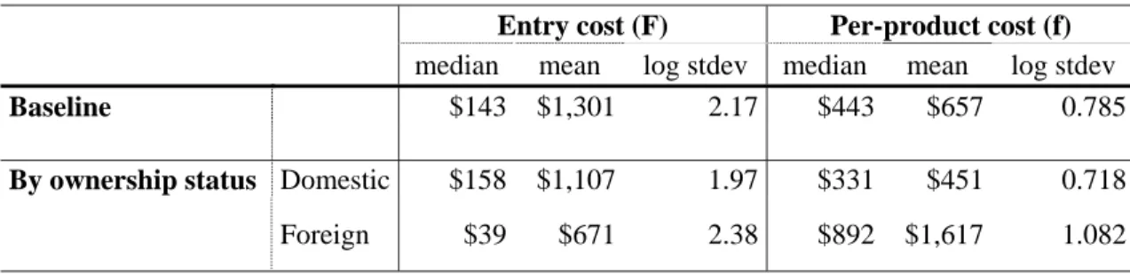
Fixed costs. Table 7 reports summary statistics for the estimated fixed cost distribution both for the baseline specification of column 1 in Table 3, and for the first specification in Table 4 which distinguishes the efficiency of import use for foreign and domestic firms. In all cases, we find that the median costs are low but dispersion across firms is high. For example, in the baseline case while the typical firm pays an entry costF of only $143, the mean entry cost is a much higher $1,301, reflecting the variance. Intuitively, our model explains the fact that many mid-sized and large firms do not import by assigning a high fixed cost to them, pulling up both the variance and the average ofF. When we distinguish firms by ownership, we find that foreign firms find it cheaper to start importing: they typical foreign firm needs to pay only $39 in contrast to the typical domestic firm which pays $158. For foreign firms, surprisingly, we also estimate a higher median fixed costf ($892 versus $331). Although, as we have shown in Fact 1, foreign firms import more kinds of products even conditional on their size, our estimates imply that this is because they gain more from imports,not because of lower average fixed costs. Intuitively, given that they find imports very productive (high
A), the only reason in our model why some foreign firms do not import a large number of varieties is that they face a high per product cost.
Finally, we measure the effect on our productivity estimates of the fixed costs of im-porting. As we discussed in Section 3.2, aγG(n) is the proper measure of the productivity gain from importing only when fixed costs are ignored. To measure the quantitative im-portance of fixed import costs, we compute, in the baseline specification, the average of
F +nf among all importers, and obtain $10,173. In contrast, the average cost saving from importing among all importers in our sample is $611,493. Thus the fixed costs account for
Table 7: Fixed costs
Entry cost (F) Per-product cost (f)
median mean log stdev median mean log stdev
Baseline $143 $1,301 2.17 $443 $657 0.785
By ownership status Domestic $158 $1,107 1.97 $331 $451 0.718
Foreign $39 $671 2.38 $892 $1,617 1.082
Notes: Summary statistics implied by our estimates for the fixed costs of importing are reported in 1991 USD. Baseline refers to specification (1) in Table 3 and By ownership status refers to specification (1) of Table 4. See Sections 4.1-4.2 and Appendix B for details.
only about 1.7 percent of the total cost savings created by imports, and as a result, ignoring them does not significantly alter the aggregate implications of our model. The reason for the small contribution of fixed costs is that much of the cost-saving from importing is realized by mid-sized and large firms importing multiple varieties. For these firms the fixed cost of importing the first few—most important—products is negligible relative to the large savings obtained through the reduction in marginal cost.
5
Applications
This section develops two applications of our estimates. In Section 5.1 we quantify the aggregate productivity effects of imports in Hungary, and in Section 5.2 we explore the implications of tariff policies in our estimated economy.
5.1
Decomposing the productivity gains in Hungary
To decompose the aggregate productivity gain in Hungary into various channels, we first write a firm’s residual log productivity ωjt = 1Fjtµ+ρjt. Here 1Fjt is an indicator for foreign
status, µis the Hicks-neutral mean log productivity premium of foreign firms, and ρjt
mea-sures remaining variation in productivity. Then the (log) productivity of firm j in year t
is φjt = [1Fjt·a F t + 1 D jt ·a D t ]·γG(njt) + 1Fjtµ+ρjt where aF
t and aDt denote the per product import gain for foreign and domestic firms in year
t and 1Djt = 1−1Fjt is an indicator for domestic firms. Following Olley and Pakes (1996), we
measure aggregate TFP as the sales-weighted average of firms’ log TFP Φt=
X
i
σjtφjt, (14)
whereσjt is the output share of firmj in yeart. Denoting by ¯GDt and ¯GFt the sales-weighted
average ofG(njt) and by σtD and σFt the sales share for domestic and foreign firms in yeart,
simple algebra shows that the growth in aggregate productivity between time t and time 0 equals Φt−Φ0