REMAINDER LINEAR SYSTEMATIC
SAMPLING WITH MULTIPLE RANDOM
STARTS
By
SAYED A. MOSTAFA ABDELMEGEED Bachelor of Science in Statistics
Cairo University Cairo, Egypt
2010
Submitted to the Faculty of the Graduate College of the Oklahoma State University
in partial fulfillment of the requirements for
the Degree of MASTER OF SCIENCE
REMAINDER LINEAR SYSTEMATIC SAMPLING WITH MULTIPLE RANDOM STARTS Thesis Approved: Dr. Ibrahim A. Ahmad Thesis Advisor Dr. Carla Goad Commitee Member Dr. Ye Liang Commitee Member
ACKNOWLEDGMENTS
I would like to thank professor Ibrahim A. Ahmad for his guidance and advice through the preparation of this work. I also would like to thank my committee members, profes-sors; C. Goad and Y. Liang for their valuable comments.
I am also thankful to professors; Laila O. El-Zeini and Ramdan Hamd for their en-couragement in the early stages of this work.
Last but not the least, I wish to thank my parents, brothers, sisters, and my wife for their support during the preparation of this work.
Acknowledgments reflect the views of the author and are not endorsed by committee members or Oklahoma State University.
Name: SAYED A. MOSTAFA ABDELMEGEED
Date of Degree: MAY, 2014
Title of Study: REMAINDER LINEAR SYSTEMATIC SAMPLING WITH
MULTI-PLE RANDOM STARTS
Abstract
“Systematic sampling, either by itself or in combination with some other method, may be the most widely used method of sampling” (Levy (2008) p.83). This fact is due to the simplicity and the operational convenience of this technique. However, this tech-nique has two main statistical problems. First, if the sampling interval,k=N/n, is not an integer, the actual sample size will not be fixed and the sample mean, ¯y, will not be unbiased estimator for ¯Y, the population mean. Second, regardless of the sampling interval, the sampling variance of the estimator ¯y cannot be consistently estimated on the basis of a single systematic sample. In this study, we introduce a new generalized systematic sampling design that can handle these two issues simultaneously. The pro-posed design is a generalization of the remainder linear systematic sampling design of Chang and Huang (2000), which handles only the problem of non-integer sampling in-tervals. Unbiased estimators for both ¯Y and the sampling variance are derived under the proposed design. The performance of the proposed design is evaluated in comparison to five sampling procedures under different supperpopulation models. Specifically, simple random sampling, remainder linear systematic sampling, circular systematic sampling, new partially systematic sampling and mixed random systematic sampling. It is found that our proposed design performs well compared to the other designs in most cases.
Contents
1. Introduction . . . 1
2. Literature Review . . . 4
2.1 Systematic Sampling Efficiency Relative to Stratified Sampling and Sim-ple Random Sampling . . . 4
2.2 Procedures for Dealing with Variable Systematic Sample Size . . . 5
2.2.1 Circular Systematic Sampling . . . 5
2.2.2 Remainder Linear Systematic Sampling . . . 6
2.3 Procedures for Estimating Systematic Sampling Variance . . . 6
2.3.1 Model Based Estimators . . . 6
2.3.2 Modifying the Linear Systematic Sampling Design . . . 8
2.3.3 Markov Systematic Sampling . . . 10
2.4 Methods Appropriate for Populations that Exhibit Certain Trend . . . . 11
2.4.1 Systematic Sampling with End Corrections . . . 11
2.4.2 Modifying the Method of Sample Selection . . . 12
2.5 Comparing Different Varieties of Systematic Sampling . . . 13
2.5.1 Comparing Procedures Handling Variable Sample Size Problem 13 2.5.2 Comparing Procedures Providing Unbiased Estimators of the Sampling Variance . . . 14
2.5.3 Comparing Systematic Sampling Schemes for Eliminating Trend Effect . . . 15
3. The Proposed Design and Estimation . . . 16
3.1 Remainder Linear Systematic Sampling with Multiple Random Starts (RLSSM) . . . 16
3.2 Estimators and their Unbiasedness . . . 17
4. Performance Comparisons . . . 23
4.1 Populations in Random Order . . . 23
4.2 Populations with Linear Trend . . . 25
4.3 Auto-correlated Populations . . . 27
4.4 On the Choice of the Number of Random Starts . . . 31
5. Conclusions and Future Work . . . 32
Glossary BSS Balanced Systematic Sampling - Sethi (1965)
BSSM Balanced Systematic Sampling with Multiple Random Starts - Sampath (2010)
CSS Circular Systematic Sampling - Lahiri (1951)
LSS Linear Systematic Sampling - Madow and Madow (1944)
MRS Multiple Random Starts
MRSS Mixed Random Systematic Sampling - Huang (2004)
MSS Modified Systematic Sampling - Singhet al.(1968)
MSSM Modified Systematic Sampling with Multiple Random Starts - Sampath (2010)
MSSS Multi-Start Systematic Sampling - Gautschi (1957)
NPSS New Partially Systematic Sampling - Leu and Tsui (1996)
NSS New Systematic Sampling - Singh and Singh (1977)
PSS Partially Systematic Sampling - Zinger (1980)
RLSS Remainder Linear Systematic Sampling - Chang and Huang (2000)
RLSSM Remainder Linear Systematic Sampling with Multiple Random Starts
SRS Simple Random Sampling
1
Introduction
Sampling design in which only the first unit is randomly selected, the rest being auto-matically selected according to a predetermined pattern is known as systematic sampling. Systematic sampling is one of the most prevalent sampling techniques. Its popularity is mainly due to its practicability. Compared to simple random sampling, it is easier to draw a sample especially when the drawing is done in the field. In addition, system-atic sampling can provide more precise estimators than simple random sampling when explicit or implicit stratification is present in the sampling frame (Cochran 1977). This is due to the fact that systematic sampling stratifies the population intonstrata each of sizekunits and selects one unit from each stratum. So, systematic sampling is expected to be about as precise as the corresponding stratified random sampling with one unit per stratum. It is also efficient in sampling some natural population like forest areas for estimating the volume of timber (Zinger 1964). Thus, many research centers use the systematic sampling design in their surveys. For example, the Food and Agriculture Or-ganization (FAO) of the United Nations utilizes systematic sampling in conducting its Global Forest Resources Assessment Survey (GFRAS 2010).
In its simplest form, called linear systematic sampling (LSS), the systematic design can be described as follows. In order to choose a systematic sample of sizenfrom a popu-lation of sizeN, the population is first divided intongroups each of sizekunits, where
k=N/n is called the sampling interval. A random start r is chosen from the first k -units group. All -units corresponding torin the remaining groups are then chosen in the sample. The obtained sample will hence comprise the units with indices;
{r,r+k,r+2k, . . . ,r+ (n−1)k}.
For instance, if N =40 and n=10, then using k=N/n=4 a random start r is first chosen from the first 4 units in the population. Letr=3, the second observation in the sample will be the unit with indexr+k=7, the third will be the unit with index 11 and so on. The sampled units in this example will be those units with indices corresponding to;
The systematic design is an equal probability of selection method. However, when the population sizeNis not a multiple of the sample sizen, the sample size will not be fixed and the sample mean becomes a biased estimator of the population mean (Kish 1965). In addition, the properties of the estimators from systematic samples depend on the order of the units in the frame, and can be less efficient under some arrangements. For in-stance, the existence of a linear or parabolic trend could produce less precise estimators. Also, if the population consists of a periodic trend like a sine curve, and the sampling interval,k, is equal to the period of the curve or an integral multiple of the period, the efficiency of a systematic sample of sizenwill be very close to that of only one obser-vation taken randomly from the population. If k is an odd multiple of the half-period, the systematic sample mean will coincide with the true population mean (Cochran 1977). Linear systematic sampling is first introduced by Madow and Madow (1944). It can be viewed as a cluster sampling where only one cluster is chosen randomly fromk clus-ters each of sizenunits. Therefore, a single systematic sample alone cannot be used to estimate the standard error of the sample mean and other sample statistics (Chaudhuri and Stenger 2005). One common practice in applied surveys is to regard LSS as a sim-ple random samsim-ple. However, such practice typically provides highly biased estimators of the sampling variance (Wolter 1984). If one is reasonably aware of the underlying model of the sampled finite population or, alternatively, the assumed infinite superpopu-lation, more appropriate estimators for the systematic sampling variance can be derived. Wolter (1984) reviewed and compared eight biased estimators for the sampling variance. Specific guidelines were then introduced based on the comparison of the mean square errors of the eight estimators under various models. Two specific estimators have been signaled as good general-purpose estimators when little is known about the population. These two estimators, denoted byv2andv3, take the following forms:
v2= (1−f) 2n(n−1) n
∑
j=2 (yj−yj−1)2 (1.1) v3= (1−f) n2 n/2∑
j=2 (y2j−y2j−1)2 (1.2)Both estimators treat the systematic sample as a special case of the stratified sample, where each stratum has 2k units and two units are chosen from each stratum using simple random sampling without replacement (SRSWOR). While v3 is based on non-overlapping differences (i.e. assumes non-non-overlapping strata), the estimatorv2is based on overlapping differences and aims at increasing the degrees of freedom (Wolter 1984). Several modifications to the LSS are introduced to tackle its main two statistical is-sues, namely, the unfixed sample size in case of non-integer sampling intervals and the difficulty of estimating the sampling variance. These modifications are reviewed below. There is still further room for modifying the LSS to deal with these two shortcomings. The proposed study introduces such approach. In this study, the focus will be on re-mainder linear systematic sampling (RLSS) of Chang and Huang (2000) where the idea of multiple random starts will be incorporated into this design in an attempt to get an
unbiased estimator for the variance of the sample mean corresponding to this design. Hence, the new developed design will be called remainder linear systematic sampling with multiple random starts (RLSSM).
Briefly, this study aims to achieve the following three main objectives:
I. Obtaining an unbiased estimator for the population mean under the proposed de-sign.
II. Estimating the variance of the sample mean unbiasedly under the proposed design. III. Investigating the performance of the proposed design relative to some other system-atic sampling designs, namely, simple random sampling (SRS), circular systemsystem-atic sampling (CSS), RLSS, new partially systematic sampling (NPSS) and mixed ran-dom systematic sampling (MRSS) through a comparative study. The comparisons will be carried out numerically in cases where the performance cannot be mathe-matically studied. Since the relative efficiencies depend on the population structure, the performance comparisons will be done under different superpopulation models. The remaining chapters of the current work are organized as follows: Chapter 2 will be devoted to reviewing background and literature. The proposed design, the estimators and their statistical properties (unbiasedness) are presented in Chapter 3. Chapter 4 includes performance comparisons of the proposed design with some other sampling designs under different superpopulation models. Conclusions and suggestions for future research are presented in Chapter 5.
2
Literature Review
This chapter introduces the systematic sampling design relative to the other common designs, namely, stratified sampling and SRS (Section 2.1). It also discusses some of the available approaches for dealing with the statistical problems of the systematic sampling design (Sections 2.2 - 2.5).
2.1
Systematic Sampling Efficiency Relative to Stratified Sampling
and Simple Random Sampling
Cochran (1977) compared the performance of the systematic sampling design with both of stratified and simple random sampling through rewriting the variance of the systematic sample mean in different ways as follows;
Var(y¯sys) = (N−1 N )S 2−k(n−1) N S 2 wsy (2.1) Var(y¯sys) = S 2 n( N−1 N )[1+ (n−1)ρw] (2.2) Var(y¯sys) = S2wst n ( N−n N )[1+ (n−1)ρwst] (2.3) Var(y¯srs) = (N−n N ) S2 n (2.4) and Var(y¯st) = ( N−n N ) S2wst n (2.5)
where,S2wsyis the variance within the systematic samples,ρwis the correlation coefficient between pairs of units that are in the same systematic sample,S2wstis the variance among units that lie in the same stratum, ρwst is the correlation between the deviations from the stratum means of pairs of items that are in the same systematic sample andVar(y¯st) is the variance of the sample mean of stratified random sample with one unit per stratum.
By comparing formulas (2.1) and (2.4), the systematic sample mean will be more effi-cient than the SRS mean ifS2wsy>S2i.e. the units within the same systematic sample are heterogeneous. Formula (2.2) shows that the existence of positive correlation between units in the same systematic sample(ρw>0)inflates the sampling variance. Hence, sys-tematic sample is less efficient than SRS if there is a positive correlation between units in the same systematic sample. Formula (2.3) relates the variance of systematic sample mean with that of stratified random sample, given in (2.5), throughρwst. Ifρwst=0, sys-tematic sampling has the same efficiency of stratified sampling with one unit per stratum. Ifρwst <0, systematic sampling is more efficient than stratified sampling with one unit per stratum. Otherwise, stratified sampling is more efficient than systematic sampling. The previous investigation shows that systematic sampling is sometimes more efficient than both of SRS and stratified sampling and sometimes it is less. In addition, the practi-cability of systematic sampling makes it more preferable design in many situations even with its other statistical shortcomings.
In the next three sections, different approaches, presented in the literature, for handling the statistical limitations of the systematic sampling design are introduced.
2.2
Procedures for Dealing with Variable Systematic Sample Size
When the population size is not a multiple of the sample size (i.e. N 6=nk) the LSS results in a variable sample size and the sample mean becomes biased as an estimator for the population mean. To overcome this drawback, many modifications on the LSS were proposed.
2.2.1 Circular Systematic Sampling
Lahiri (1951) suggested a sampling design where the units of the population are con-sidered to be arranged around a circle. In such case, instead of dividing the population intongroups and selecting a random number from the first group, as in LSS, a random numberris selected between 1 to N. Everykth unit is then chosen in a cyclic manner to be in the sample, wherek= [N/n], the integer part ofN/n, is the sampling interval. This design is based on the convention that for anyi=1,2, . . . ,N, the unit with index i+N
stands for the unit with indexi, and hence this design is known as circular systematic sampling (CSS). The units in the sample are those with indices;
r+jk if 1≤r+ jk≤N
r+jk-N if r+jk>N ; j=0,1, . . . ,(n−1)
Under this design an unbiased estimator for the population mean can be obtained as follows:
¯
Sudakar (1978) pointed out that to achieve the required sample sizenin CSS,kshould be chosen as the largest integer smaller than or equal toN/n.
Sengupta and Chattopadhyay (1987) mentioned that a necessary and sufficient condition to make the CSS of size n, drawn from a population of N units with sampling inter-val k, contain all distinct units is that N/(N,k)≥nor equivalently, [N,k]/k≤n, where (N,k)and[N,k]denote, respectively, the greatest common divisor (g.c.d) and least com-mon multiple (l.c.m) ofN andk.
Like the usual LSS, the CSS design does not provide an unbiased estimator for the sampling variance of the sample mean.
2.2.2 Remainder Linear Systematic Sampling
Chang and Huang (2000) proposed another sampling procedure that can be used when
N=nk+r; 0<r<n. This procedure is based on the fact that the population size can be written asN= (n−r)k+r(k+1), which means that the population can be divided into two strata, the first consists of the front(n−r)k units, and the second stratum contains the remainingr(k+1)units. A linear systematic sample of size(n−r)units is selected from the first stratum with k as the sampling interval, and another linear systematic sample of sizer units is selected from the second stratum with(k+1)as the sampling interval. Combining the two samples together, we get a sample of sizenas desired. This design is called remainder linear systematic sampling (RLSS). It is reduced to LSS if the remainder is zero,r=0. Under the RLSS, an unbiased estimator for the population mean can be obtained as follows:
¯
yRLSS =N1[(n−r)ky¯1+r(k+1)y¯2]
where, ¯y1 and ¯y2 are the sample means of the first and second stratum, respectively. However, under this design there is no unbiased estimator for the sampling variance.
2.3
Procedures for Estimating Systematic Sampling Variance
As it is mentioned above, a single systematic sample cannot be used solely to estimate the variance of the sample mean, or any other sample statistic of interest, unbiasedly. This issue can be tackled using one of several approaches presented in literature. The following is a review of such approaches.
2.3.1 Model Based Estimators
This approach is based on assigning a model that best characterizes the nature of the values of the variable of interest when they are arranged in certain order. For example, several model-based estimators are given in Cochran (1977, p.223). Each of these esti-mators is approximately unbiased under a specific underlying model but can be highly
biased under the other models. Therefore, the researcher should be careful while choos-ing the estimator to be used. The golden rule would be to avoid uschoos-ing LSS if the under-lying model of the sampled population is unknown (Wolter (2007)).
Montanari and Bartolucci (1998) proposed a model-based estimator of the variance of the systematic sample mean that is based on a sum of two components. The first com-ponent takes into account the trend in the frame of the sampled finite population while the second takes into account the stochastic nature of a general superpopulation model. Given thatyi jis the value of the study variableY of the jthunit in theith systematic sam-ple, they assumed thatyi j is a realization of the random variableY under the following superpopulation model:
yi j=µi j+εi j
EM(yi j) =µi j, VM(yi j) =σi j2, CovM(yi j,yi0j0) =0 ∀i6=i0or j6= j0
They showed thatEM[Var(y¯sys)]can be divided into two parts where the first part is due to the systematic component and the other is due to the random component of the as-sumed model. Based on this idea, they introduced their model based estimator. Their estimator was shown to outperform both the overlapping difference estimatorv2 (equa-tion 1.1) and the simple random sample estimator under several superpopula(equa-tion models. Wolter (2007, sec. 8.2.2) proposed a general methodology for constructing a model based estimator forVar(y¯). In this methodology, the model dependence is explicitly recognized. The proposed general estimator of the variance is defined as a conditional expectation ofVar(y¯)given the datayifrom the observed sample;
vi=E[Var(y¯)|yi]
where,Edenotes the expectation over the assumed specific model.
In this context, Wolter (2007) notes that the practicing statistician must make a pro-fessional judgment about the form of the model, as it is never known exactly, and then deriveviunder the selected form. Hence, the variance estimator will be subject to errors of estimation as well as to errors of model specification. Therefore, the applicability of the model based approach is viewed, in practice, as being hampered by lack of robust-ness.
This lack of robustness can be partly handled by the use of a nonparametric model speci-fication. This class of models, compared to parametric models, makes much less restric-tive assumptions on the shape of the relationship between variables which significantly reduces the risk of model misspecification.
the design variance under a nonparametric model for the population. They derived their estimator under the following superpopulation model:
Yj=m(xj) +v(xj)1/2ej; 1≤ j≤N (2.6) where m(.) andv(.) are continuous and bounded functions, x is a univariate auxiliary variable and the errorsejare independent random variables with mean 0 and variance 1. The design variance of ¯yis then written as follows:
Vard(y¯) = 1k∑kr=1(y¯r−Y¯)2= kn12YTDY
where,Y = (Y1, . . . ,YN)T andD=ETHE withE=1Tn⊗Ik, H=Ik−1k1k1Tk,⊗denoting the Kronecker product1 and 1k a vector of ones of length k. The model anticipated variance of ¯yunder the assumed model, in (2.6), is then defined as follows:
E[Vard(y¯)] = 1
kn2mTDm+
1
kn2tr(DΣ)
where, m= [m(x1), . . . ,m(xN)]T and Σ=diag[var(x1), . . . ,var(xN)]. This anticipated variance is then estimated using the local polynomial regression.
2.3.2 Modifying the Linear Systematic Sampling Design
Instead of depending on a model based estimator to estimate the systematic sampling variance, many authors suggested to modify the design itself in a way that enables the derivation of unbiased estimators for the sampling variance. Some of these modifica-tions are reviewed below.
a. Mixed Random Systematic Sampling Designs
In this approach, a systematic sample is first chosen from the population and then supple-mented with an additional simple random sample without replacement or with another systematic sample from the remainder of the population. The two samples are then used to provide an unbiased estimator for the variance of the estimator of the population mean. This approach, with some variations, is adopted by many authors.
Zinger (1980) introduced the partially systematic sampling (PSS) design in an attempt to provide an unbiased estimator for the sampling variance. This design can be described as follows:
To select a sample of sizen from a population of size N =mk, where m<n, a linear systematic sample of sizemunits is first chosen. A simple random sample (SRS) of size
1Kronecker product⊗: LetA∈R(mn)andB∈R(pq). Then the Kronecker product ofAandBis defined
as the matrix;A⊗B= a11B · · · a1nB .. . . .. ... am1B · · · amnB ∈R (mp×nq)(Hadi 1996).
(n−m)units is then selected from the remaining (N−m)units. The final sample will be the union of the two samples. To estimate the population mean ¯Y, a weighted sample mean can be used as follows; ¯yw=αy¯sys+βy¯srs, with α,β ≥0 and α+β =1. This procedure appears to provide an unbiased estimator for the sampling variance through the sample sum of squares.
Singh and Singh (1977) proposed the new systematic sampling (NSS) design where choosing a sample of sizeninvolves two steps. First, a sample ofuconsecutive units is selected by choosing a random numbertbetween 1 andN. A circular systematic sample of size(n−u)units is then selected using sampling intervalk=N/n. The sampled units are those with indices;
{t+i;i=0,1,2, . . . ,u−1} & {t+u−1+jk;j=1,2, . . . ,n−u}.
A sufficient condition to guarantee that the sampled units will be distinct isu+(n−u)k≤
N. They also mentioned that another sufficient condition which should be added to make all the pairs of units have non-zero inclusion probabilities, and hence the sampling vari-ance can be estimated unbiasedly, isu≥kandu+ (n−u)k≥ 12N+1.
Leu and Tsui (1996) modified the NSS of Singh and Singh (1977) by suggesting new partially systematic sampling (NPSS) design. The new design modifies the NSS by choosing a random sample of sizeafrom the indices;
{t,t+1, . . . ,t+u−1}
where, u=N−(n−a)k anda=2 ifN=nk; otherwise,k= [N/(n−1)]and 2≤a≤
[N/2] +1. A systematic sample of size (n−a) is then chosen, in a circular manner, which includes the units with indices;
{t+u−1+jk;j=1,2, . . . ,(n−a)}.
Combining the two samples together, a sample of sizencan be formed from which an unbiased estimator for the sampling variance can be obtained provided thata≥2 and
u≥k, through utilizing the second order inclusion probabilities.
Huang (2004) proposed a mixed random systematic sampling (MRSS) design from which both the population mean and the sampling variance can be estimated unbiasedly. Considering the population as if arranged in a circular manner, the proposed design in-volves two steps. In the first step an index t is selected randomly between 1 and N. Then the population is divided into two subpopulations; the first consists of (n−r)k
units with indices{t,t+1, . . . ,t+ (n−r)k−1}and the second subpopulation contains
r(k+1)units with the remaining indices. In the second step, a simple random sample of size(n−r)is drawn from the first subpopulation and a sample of runits, with indices
{t+ (n−r)k−1+j(k+1);j =1,2, . . . ,r} is selected systematically from the second one. The final sample is then the union of the two samples. If N =nk, MRSS will be equivalent to SRS. Under the proposed procedure, the inclusion probabilities were
derived and the Horvitz-Thompson (HT) estimator was used to estimate the population mean.2 Also, an unbiased estimator for the variance of the HT estimator was presented by utilizing the second order inclusion probabilities.
It is noteworthy that the last three methods, namely, NSS, NPSS and MRSS can also be used when the population size is not a multiple of the sample size(N 6=nk)as their introducers, Singh and Singh (1977), Leu and Tsui (1996) and Huang (2004), respec-tively, mentioned.
b. Multi-Start Systematic Sampling
Gautschi(1957) proposed LSS with multiple random starts aiming at providing an un-biased estimator for the systematic sampling variance. According to this approach, in order to select a systematic sample of sizen, one choosest independent systematic sub-samples. ForN=nkandn/t is integer, we first choosetrandom numbers from the front
tk units (the first group), say{r1, . . . ,rt}. Then for each chosen random start, a system-atic sample is selected by choosing the correspondingtkthunits. Finally, the sample will contain units with the following indices;
{r1,r1+tk, . . . ,r1+ (nt −1)tk, . . . ,rt,rt+tk, . . . ,rt+ (nt −1)tk}.
This design is called a multi-start systematic sampling (MSSS). An unbiased estimator for the sampling variance can be obtained as;
ˆ
Var(y¯) =t(1t−−f1)∑ti=1(y¯i−y¯)2= t(t−k−11)k∑it=1(y¯i−y¯)2,
where, f =n/N, ¯y=1t ∑ti=1y¯iand ¯yiis the subsample mean.
The approach of multiple random starts (MRS) has been incorporated into different sys-tematic sampling methods in order to derive unbiased estimators for the variance of the proposed new estimators of the population mean (see, sec. 2.4.2).
2.3.3 Markov Systematic Sampling
Sampath and Uthayakumaran (1998) introduced a new sampling scheme with Markovian behavior which yields positive inclusion probabilities for all pairs of units. This sam-pling scheme overcomes the difficulties in Markov samsam-pling proposed by Chandraet al.
(1991). Markov systematic sampling procedure assumes that the sample size is even and the population size is a multiple of the sample size (i.e. k=N/nis an integer). The pop-ulation is divided inton/2 groups in a systematic manner, sayS1, . . . ,Smwherem=n/2 and theith group(Si)includes those units with indices{2(i−1)k+ j;j=1,2, . . . ,2k}. For each group Si, define a transition probability matrix (TPM) Ai of a Markov chain with state space{2(i−1)k+j;j=1,2, . . . ,2k}. To guarantee that all the sampled units
2The general form for the Horvitz-Thompson estimator for the population mean is given by ¯y= 1
N∑i∈syπii, whereπiis the inclusion probability of thei
will be distinct, the diagonal elements in eachAishould be zero,i=1,2, . . . ,m. Select-ing a sample of sizenusing this procedure involves two steps. First, a random number
ris drawn from 1 to 2k. A systematic sample of sizem=n/2 is then selected using 2k
as the sampling interval. The units with indices{r,r+2k, . . . ,r+2(m−1)k}will be the selected units. A single unit is then drawn from each group independently using the el-ements ofAias conditional probabilities. They assumed that the non-diagonal elements of the TPMAi(ars) are selected so that for eachr;
ars∝τ|r−s|,s=1,2, . . . ,2k,
whereτ is a predetermined positive number which can be chosen either to be the same
for all TPMs or to be differentτ for the different TPMs. If the sameτ is used, we will
have a common TPM, say A. The sampling variance can be estimated with the help of the Horvitz-Thompson estimator since all the pairs of units have non-zero inclusion probability.
Kaoet al. (2011) proposed the remainder Markov systematic sampling design that ex-tends the RLSS and Markov systematic sampling in an attempt to solve the two main statistical problems of the LSS simultaneously. According to their design, selecting a sample of sizeninvolves the following two steps.
1. Divide the population into two strata; the first stratum contains the front(n−r)k
units and the second stratum contains the remainingr(k+1)units. 2. Apply the Markov systematic sampling method to each stratum.
2.4
Methods Appropriate for Populations that Exhibit Certain
Trend
In literature there are several ways to improve the performance of systematic sampling in the presence of a linear or parabolic trend in the population. One way is to use a weighted mean instead of the unweighted one (usual sample mean ¯y). On the other hand, one may change the method of sample selection so that the sample mean is not affected by the presence of certain trend. Such two approaches are discussed below in details.
2.4.1 Systematic Sampling with End Corrections
Yates (1948) suggested using a weighted mean in which all internal units of the sample have weight unity (before multiplying byn−1) but the first and last units have different weights. If the random number selected between 1 andkisr, the weights of the first and last unit are
1±n(22(r−k−n−1)k1).
¯
yw=y¯+22r−k−(n−1)1k(yr−yr+(n−1)k)
It can be easily verified that if the population consists solely of a linear trend andN=nk, the suggested weighted mean coincides with the true population mean.
Bellhouse and Rao (1975) applied the Yates end corrections to the CSS of Lahiri (1951) to improve its performance in the presence of linear trend. Two cases arise while esti-mating the population mean as follows:
Case 1. The random start taken between 1 andNis small enough,r+ (n−1)k≤N. The weights for the first and last unit selected in the sample are
1±n[2r+(2n−(n−1)k−1)k(N+1)].
As before, the+sign is used for the first unit, the−sign for the last.
Case 2. The random start taken between 1 andNis large enough,r+ (n−1)k>N. Letn2be the number of sampled units obtained after passing theNth unit in the popula-tion. Then the weights are defined as
1±[2nr+n(n−1)k−n(N+1)−2n2N]
2(N−k) .
The+sign is still used for the first unit, the−sign for the last.
2.4.2 Modifying the Method of Sample Selection
Sethi (1965) proposed the balanced systematic sampling (BSS) scheme. With N=nk
andn is even, the population is first divided inton/2 strata each of size 2k. Two units equidistant from the end of each stratum are selected in the sample. If the selected random start is 1≤r≤2k, the sampled units will have the following indices:
[r+2jk, 2(j+1)k−r+1] ; j=0,1, . . . ,n2−1 Withnodd, the sample will be
[r+2jk, 2(j+1)k−r+1, r+ (n−1)k] ; j=0,1, . . . ,(n−21)−1
Singhet al.(1968) proposed the modified systematic sampling design (MSS) that can be used for populations exhibiting linear trend. To choose a sample of even sizenusing this design, we first select a random numberrfrom 1 tok. Then, each pair of units equidistant from the ends of the population is drawn systematically. The sample corresponding to the random start 1≤r≤k, will contain the units with indices;
Withnodd, the sample will be
[r+jk, N−r−jk+1, r+12(n−1)k] ; j=0,1, . . . ,(n−21)−1.
Madow (1953) introduced a centered systematic sampling scheme in which the random startr is taken as k2 or k+22 for even k0s and k+21 for oddk0s. This means that we select the cluster in the center of the possiblekclusters.
Sampath and Ammani (2010) applied the MRS approach to the BSS due to Sethi (1965) and the MSS of Singh et al. (1968) to provide an unbiased estimator for the sampling variance under these designs. The new designs are described in the following:
I. Balanced Systematic Sampling with Multiple Random Starts (BSSM)
To select a sample of sizenusing BSSM design withtrandom starts, one can proceed as follows. First, the population is divided inton/2t groups each of 2tkunits. Thent ran-dom numbers are selected from 1 totk. Corresponding to every random number chosen, pairs of units equidistant from the group ends are selected in the sample. Clearly, each random number contributesn/t units to the sample. Therefore, the sample will contain
nunits. Under this design, the sample mean was proved to be an unbiased estimator for the population mean. It was also proved to coincide with the population mean in the presence of linear trend.
II. Modified Systematic Sampling with Multiple Random Starts (MSSM)
When the sample is desired to be selected using MSSM design, then instead of choosing one random start,t random starts are chosen between 1 andtk. Corresponding to every random start selected, pairs of units equidistant from the population ends are selected in the sample in a systematic manner. The sample corresponding to the random start
ri; i=1,2, . . . ,t, will consist of then/tunits with indices;
[ri+ jtk, N−ri−jtk+1] ; j=0,1, . . . ,2nt−1.
The population mean is estimated unbiasedly under this design using the sample mean.
2.5
Comparing Different Varieties of Systematic Sampling
In this section comparisons of different versions of systematic sampling are introduced in the sake of highlighting their relative performance.
2.5.1 Comparing Procedures Handling Variable Sample Size Problem
Chang and Huang (2000) assessed the performance of the RLSS relative to SRS, CSS and NPSS under various types of populations and they mentioned the following conclu-sions:
a. For populations in random order, the RLSS is more efficient than SRS if and only if the sample proportion of the second stratum is larger than the second stratum variance proportion.
b. For populations exhibiting linear trend,Yi=i;i=1,2, . . . ,N, the RLSS outperforms SRS ifNis not a multiple of the sample size.
c. The RLSS is more efficient than SRS and NPSS for the three types of autocorre-lated populations, namely, populations with linear, exponential and hyperbolic correl-ogram. Also, the RLSS outperforms the CSS for populations with linear correlogram and they are equally efficient for the other types.
2.5.2 Comparing Procedures Providing Unbiased Estimators of the Sampling Variance
Zinger (1980) compared the PSS design with the multi-start systematic sampling. The PSS design is proved to outperform the MSSS if ρw >0 andt =2 or 3, or if ρw<0 andt ≥4, wheret is the number of random starts and ρw is the correlation coefficient between pairs of units that are in the same systematic sample.
Leu and Tsui (1996) compared the NPSS with some other sampling procedures under different types of superpopulation. They concluded that:
a. For populations in random order, the NPSS, LSS and SRS are equally efficient. b. For the auto-correlated populations - linear, exponential and hyperbolic
correlogram-NPSS is more efficient than SRS. But correlogram-NPSS is less efficient than CSS and LSS pro-cedures. In most of the cases, the NPSS outperforms the systematic sampling with multiple random starts.
c. For populations with periodic variation, NPSS is more efficient than LSS. In these populations, the efficiency of the LSS depends on the sampling interval k as men-tioned above.
Huang (2004) investigated the performance of the MRSS relative to SRS, CSS and NPSS under different types of population. Huang concluded that:
a. The four designs are equally efficient for populations in random order.
b. For populations with linear trend,Yi=α+β(i), the MRSS is consistently more
effi-cient than SRS, and more effieffi-cient than CSS and NPSS in some cases.
c. For the auto-correlated populations, the results are similar to those of the populations with linear trend.
Gautschi (1957) compared the MSSS with the LSS under different types of populations and concluded that the MSSS is more efficient in most cases. Hence, the researcher is
better off choosing MSSS as it provides an unbiased estimator for the sampling variance. Sampath and Ammani (2010) assessed the performance of both BSSM and MSSM rel-ative to each other and relrel-ative to the MSSS under the model that is suitable for popula-tions with linear trend. The model is as follows;
Yi=α+β(i) +ei
where,E(ei) =0,V(ei) =σ2(i)gandCov(ei,ej) =0 ∀i6= j. They concluded that:
a. The proposed designs were proved to provide estimators for the population mean that coincide with this mean in the presence of linear trend i.e. they estimate the population mean without any error.
b. For all choices ofgandn, BSSM and MSSM are equally efficient as long as we use two random starts.
c. For all choices ofgandn, BSSM and MSSM are more efficient than MSSS.
Sampath and Uthayakumaran (1998) compared Markov systematic sampling with SRS, LSS, stratified random sampling and systematic sampling with two random starts for the populations exhibiting exponential trend. For the deterministic exponential model (Yi =βi;i= 1,2, . . . ,N), Markov systematic sampling has been found to outperform
the other procedures. Also, the estimator under Markov systematic sampling is more efficient than the estimators under LSS and systematic sampling with two random starts for populations exhibiting approximate exponential trend (Yi=βi+ei;i=1,2, . . . ,Nand
E(ei) =0,E(ei2) =σ2,E(eiej) =0∀i6= j) whenτ>1.2,β >1 andσ2<75.
2.5.3 Comparing Systematic Sampling Schemes for Eliminating Trend Effect
Bellhouse and Rao (1975) assessed the performance of both centered systematic sam-pling, BSS and MSS relative to LSS with Yates corrections and LSS under superpopu-lation models representing linear and parabolic trends and periodic and autocorrelated variations. In the presence of a linear or parabolic trend, all the three methods, Yates corrections, BSS and MSS, outperform the ordinary LSS.
After reviewing the systematic sampling approach and its derivative designs proposed to handle one or more of the mentioned statistical issues involved in this design, we shall introduce our proposed design in the following chapter. In this chapter, Chapter 3, the proposed design and estimators for the population mean and the sampling variance under this design will be introduced.
3
The Proposed Design and Estimation
The proposed design is a systematic sampling scheme which is a multiple random starts analogue of RLSS. Unbiased estimators for both the population mean and the sampling variance are derived under the proposed design. The following presents this design and the derivations of the estimators in details.
3.1
Remainder Linear Systematic Sampling with Multiple
Random Starts (RLSSM)
According to the RLSS design, the population can be divided into two strata; the front (n−r)kunits as a stratum and the remainingr(k+1)units as another stratum, as men-tioned in Section 2.2.2. Based on this idea, our proposed RLSSM design proceeds as follows:
a. For the first stratum:
Select 1<t1<(n−r)different random numbers from the frontt1kunits such that (n−rt )
1
is integer;
1≤C1,C2, . . . ,Ct1 ≤t1k.
Then for each random number chosen select a systematic sample by addingt1k as the sampling interval. The sampled units will be;
S0={yCi+(l0−1)t
1k ; i=1,2, . . . ,t1, l
0=1,2, . . . ,(n−r)
t1 }
b. For the second stratum:
Select 1<t2<rdifferent random numbers from[(n−r)k+1]to[(n−r)k+t2(k+1)] such that tr
2 is integer;
1≤C1,C2, . . . ,Ct2≤t2(k+1)
Then for each random number chosen select a systematic sample by addingt2(k+1)as the sampling interval. The sample will be;
S00={y(n−r)k+Ci+(l00−1)t
2(k+1) ; i=1,2, . . . ,t2, l
00=1,2, . . . , r t2}
The desired sample will be the union ofS0andS00and of sizen= (n−r) +r.
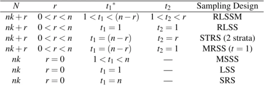
It is worth noting that the proposed design can be considered as a generalized systematic sampling design. This note is due to the fact that four other designs can be obtained as special cases of the proposed one. Moreover, two special cases of other designs can be obtained as special cases of RLSSM design. Table (1) shows the relations between RLSSM design and the other designs.
Table 1. RLSSM design and its special cases.
N r t1∗ t2 Sampling Design nk+r 0<r<n 1<t1<(n−r) 1<t2<r RLSSM nk+r 0<r<n t1=1 t2=1 RLSS nk+r 0<r<n t1= (n−r) t2=r STRS (2 strata) nk+r 0<r<n t1= (n−r) t2=1 MRSS (t=1) nk r=0 1<t1<n — MSSS nk r=0 t1=1 — LSS nk r=0 t1=n — SRS
*t1andt2are selected such that (n
−r) t1 and
r
t2 are integers, respectively.
From Table (1), RLSS design is just a RLSSM whent1=t2=1 i.e. only one random start is taken from each subpopulation. Also, forr=0 our proposed design can produce one of three different designs depending ont1, the number of random starts. If 1<t1<n, our design will be reduced to MSSS. On the other hand, ift1is one of its two extremes,
t1=1 ort1=n, the produced design will be either LSS or SRS, respectively.
Additionally, a special case of MRSS design of Huang (2004) where the random start
t =1 can be obtained from RLSSM whent1= (n−r)andt2=1. In the former case, if
t2=r instead of 1, the proposed design wil be equivalent to a stratified random sample of sizenwith only two strata.
3.2
Estimators and their Unbiasedness
Based on the two samples, one can estimate the population mean ¯Y as follows:
Step 1.Estimate the first subpopulation mean ¯Y1based on the sampleS0using the sample mean in the form,
¯ y1= (n−r1 )∑ti=1 1∑(l0n−r=1)/t1yci+(l0−1)t1k ¯ y1= (n−r1 )∑it1=1(n−rt1 )y¯i where ¯ yi= t1 (n−r)∑ (n−r)/t1 l0=1 yci+(l0−1)t1k
Thus, ¯ y1= 1 t1 t1
∑
i=1 ¯ yi (3.1)Step 2. Estimate the second subpopulation mean ¯Y2 based on the sampleS00 using the sample mean in the form,
¯ y2= 1r∑ti2=1∑rl00/=t21y(n−r)k+ci+(l00−1)t2(k+1) ¯ y2= 1r∑it2=1tr2y¯i where ¯ yi= tr2∑lr00/=t21y(n−r)k+ci+(l00−1)t2(k+1) Thus, ¯ y2= 1 t2 t2
∑
i=1 ¯ yi (3.2)Step 3. The estimator of the population mean can be taken as a weighted mean of the two means stated above in (3.1) and (3.2):
¯
yRLSSM=
(n−r)ky¯1+r(k+1)y¯2
N (3.3)
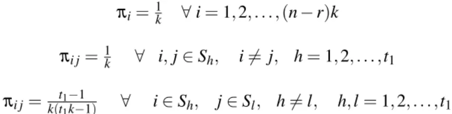
Lemma1: Under this design (RLSSM) the first and second order inclusion probabilities for units in the first subpopulation [1 to(n−r)k] are defined as follows:
πi= 1k ∀i=1,2, . . . ,(n−r)k
πi j = 1k ∀ i,j∈Sh, i6= j, h=1,2, . . . ,t1
πi j= k(tt11−k−11) ∀ i∈Sh, j∈Sl, h6=l, h,l=1,2, . . . ,t1
Proof: Let us look at thet1-start systematic sample chosen from the first subpopulation from another side following Sampath (2012). To choose a sample of size(n−r)from that population, it is first divided intot1kgroups of(n−r)/t1units each, as in Table (2), andt1of these groups will be randomly selected to get the desired sample.
Table 2. Partitioning the first subpopulation under MSSS. Units S1 1 t1k+1 2t1k+1 . . . [(n−r)/t1−1]t1k+1 S2 2 t1k+2 2t1k+2 . . . [(n−r)/t1−1]t1k+2 . . . . . . . . Groups Si i t1k+i 2t1k+i . . . [(n−r)/t1−1]t1k+i . . . . . . . . St1k t1k 2t1k 3t1k . . . (n−r)k
The probability of including the unit with labeliin the sample(πi)is exactly the proba-bility of including the group containing this unit in the sample. Therefore, the first order inclusion probabilities can be defined as follows:
πi=tt11k = 1k ∀i=1,2, . . . ,(n−r)k
Following the same view, it should be noticed that the second order inclusion proba-bilities for pairs of units which belong to the same group are equal to the probability of selecting this group in the sample which is equal to the first order inclusion probabilities. On the other hand, if the pair of units belongs to two different groups, then including this pair in the sample can be only realized by selecting the two groups in the sample. Hence, the second order inclusion probability in this case will be:
πi j= tt11k∗tt11k−−11 =k(tt11−k−11) ∀ i∈Sh, j∈Sl, h6=l, h,l=1,2, . . . ,t1 The proof is complete.
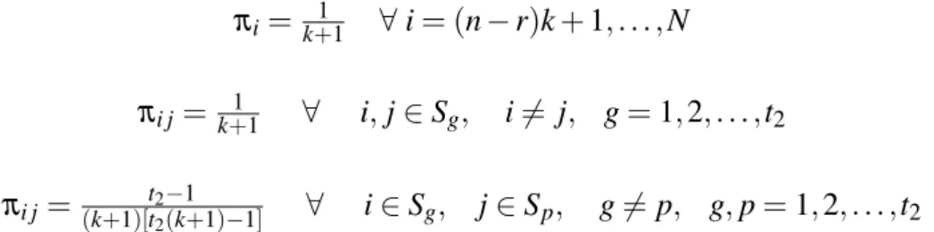
Lemma2: Under this design (RLSSM) the first and second order inclusion probabilities for units in the second subpopulation [(n−r)k+1 toN] are defined as follows:
πi= k+11 ∀i= (n−r)k+1, . . . ,N
πi j= k+11 ∀ i,j∈Sg, i6= j, g=1,2, . . . ,t2
πi j = (k+1)[tt22(−k1+1)−1] ∀ i∈Sg, j∈Sp, g6=p, g,p=1,2, . . . ,t2
Proof: To choose a sample of sizerfrom the second subpopulation, this population is first divided intot2(k+1) groups of(r/t2) units each, as in Table (3), andt2 of these groups will be randomly selected to get the desired sample.
Table 3. Partitioning the second subpopulation under MSSS. Units S1 1 t2(k+1) +1 2t2(k+1) +1 . . . [r/t2−1]t2(k+1) +1 S2 2 t2(k+1) +2 2t2(k+1) +2 . . . [r/t2−1]t2(k+1) +2 . . . . . . . . Groups Si i t2(k+1) +i 2t2(k+1) +i . . . [r/t2−1]t2(k+1) +i . . . . . . . . St2(k+1) t2(k+1) 2t2(k+1) 3t2(k+1) . . . r(k+1)
The rest of the proof follows the same procedure used in the proof of Lemma 1.
Theorem1: The sample mean of the RLSSM design, ¯yRLSSM, is an unbiased estimator for the population mean ¯Y.
Proof: Since, ¯y1and ¯y2are unbiased estimators for the subpopulation means, ¯Y1and ¯Y2, respectively, (Gautschi (1957)), then
E(y¯RLSSM) = (n−r)kY¯1+r(k+1)Y¯2 N = ∑ (n−r)k j=1 Yj+∑Nj=(n−r)k+1Yj N = N1∑Nj=1Yj=Y¯. This proves the theorem.
Remark 1: It can be easily shown that the proposed estimator (y¯RLSSM) is in fact a Horvitz-Thomson (1952) estimator in the form ˆ¯YHT = N1 ∑ui∈Sπyii as follows:
¯ yRLSSM= N1[(n−r)k.n−r1 ∑ti1=1∑ n−r t1 l0=1yci+(l0−1)t1k +r(k+1).1r∑ti2=1∑ r t2 l00=1y(n−r)k+ci+(l00−1)t2(k+1)] =N1[∑ti1=1∑ n−r t1 l0=1 yci+(l0−1)t 1k 1/k +∑ t2 i=1∑ r t2 l00=1 y(n−r)k+ci+(l00−1)t 2(k+1) 1/(k+1) ] =N1[∑Ui∈S0 yi πi+∑Uj∈S00 yj πj].
Therefore, an unbiased estimator for the sampling variance can be derived based on Yates - Grundy (1953) estimator which has the following form;
ˆ Var(y¯n) = 1 N2∑ n i=1∑nj>i (πiπj−πi j) πi j ( yi πi− yj πj) 2
However, the terms(πiπj−πi j)are sometimes negative under the proposed design and so ˆVar(y¯n)may be sometimes negative. Thus the sampling variance of this design and another unbiased estimator that is always positive are given by the following two theo-rems.
Theorem2: Under the RLSSM design, the variance of the sample mean has the form:
Var(y¯RLSSM) = 1 N2{ (n−r)2k(k−1) t1(t1k−1) t1k
∑
i=1 (Y¯1i−Y¯1)2+ r 2k(k+1) t2[t2(k+1)−1] t2(k+1)∑
i=1 (Y¯2i−Y¯2)2} (3.4) Proof: Since, the random starts are chosen independently, ¯y1 and ¯y2 are independent.Var(y¯RLSSM) = 1 N2[(n−r)2k2.Var(y¯1) +r2(k+1)2.Var(y¯2)] = 1 N2{(n−r) 2k2(1−1 k) s12 t1 +r 2(k+1)2(1− 1 k+1) s22 t2 } (3.5) where, S12= t 1 1k−1∑ t1k
i=1(Y¯1i−Y¯1)2 is the variance between clusters’ means in the first stratum andS22= t 1
2(k+1)−1∑
t2(k+1)
i=1 (Y¯2i−Y¯2)2is the variance between clusters’ means in the second stratum.
Substituting these quantities in (3.5), the theorem follows.
Theorem3: The sampling variance of the RLSSM design can be estimated unbiasedly as follows: ˆ Var(y¯RLSSM) = 1 N2{ (n−r)2k(k−1) t1(t1−1) t1
∑
j=1 (y¯1j−y¯1)2+r 2k(k+1) t2(t2−1) t2∑
j=1 (y¯2j−y¯2)2} (3.6)where, ¯y1j ;j=1, . . . ,t1 is the mean of the jth sample from the first subpopulation and ¯
y2j;j=1, . . . ,t2is the mean of the jthsample from the second subpopulation. Proof:Since it can be proved that ˆS12=t 1
1−1∑ t1 j=1(y¯1j−y¯1)2and ˆS2 2= 1 t2−1∑ t2 j=1(y¯2j− ¯
y2)2are unbiased estimators forS12andS22respectively, as follows;
E(Sˆ12) = t 1 1−1E[∑ t1 j=1(y¯1j−y¯1)2] = t 1 1−1E∑ t1 j=1[(y¯1j−Y¯1)2+ (y¯1−Y¯1)2−2(y¯1j−Y¯1)(y¯1−Y¯1)] =t 1 1−1E[∑ t1 j=1(y¯1j−Y¯1) 2−t 1(y¯1−Y¯1)2] =t 1 1−1[t1( 1 t1k)∑ t1k i=1(Y¯1i−Y¯1)2−t1( k−1 t1k )( 1 t1k−1)∑ t1k i=1(Y¯1i−Y¯1)2] =t 1 1−1[ 1 k∑ t1k i=1(Y¯1i−Y¯1) 2(1− k−1 t1k−1)] = 1 t1k−1∑ t1k i=1(Y¯1i−Y¯1) 2=S 12
Using similar procedure, ˆS22is an unbiased estimator forS22. This completes the theo-rem.
3.3
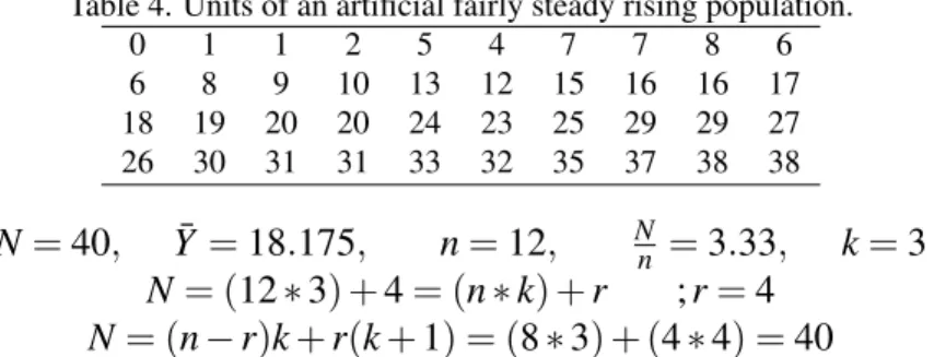
A Numerical Illustration for RLSSM Procedure
Consider the population of size 40 units given in Cochran (1977, p.211, Table 8.3) which is an artificial population that exhibits a fairly steady rising trend. If the population mean is needed to be estimated on the basis of a sample of size 12 units, using RLSSM one can proceed as follows:
Table 4. Units of an artificial fairly steady rising population. 0 1 1 2 5 4 7 7 8 6 6 8 9 10 13 12 15 16 16 17 18 19 20 20 24 23 25 29 29 27 26 30 31 31 33 32 35 37 38 38 N=40, Y¯ =18.175, n=12, Nn =3.33, k=3 N= (12∗3) +4= (n∗k) +r ;r=4 N= (n−r)k+r(k+1) = (8∗3) + (4∗4) =40
From the first subpopulation, 1,2, . . . ,(n−r)k=24,select a multi-start systematic sam-ple of size 8 units usingt1 =2 random starts. Let the first random start chosen from 1,2, . . . ,t1k=6, beC1=4 then,
S10={y4,y10,y16,y22}. IfC2=2,
S20={y2,y8,y14,y20} and the sample from the first subpopulation will be:
S0={y2,y4,y8,y10,y14,y16,y20,y22}={1,2,7,6,10,12,17,19}. Thus,
¯
y1= 9.75+28.75 =9.25.
From the second subpopulation,(n−r)k+1=25, . . . ,N=40,select a multi-start sys-tematic sample of size 4 units using t2 =2 random starts. Let the first random start chosen from 25,26, . . . ,(n−r)k+t2(k+1) =32, beC1=29 then,
S100={y29,y37}. IfC2=26,
S200={y26,y34}
and the sample from the second subpopulation will be:
S00={y26,y29,y34,y37}={23,29,31,35}. ¯ y2= 32+227 =29.5 ¯ yRLSSM=17.35 ˆ Var(y¯RLSSM) =0.81
If these 12 units are selected randomly, SRS; ¯
ySRS= 19212 =16 ˆ
Var(y¯SRS) =7.254
4
Performance Comparisons
Efficiencies of systematic sampling designs depend on the characters of the sampled populations. Thus, efficiencies of these sampling procedures are compared for various types of populations. Instead of considering a single finite population,y1, . . . ,yN, it will be assumed, following Cochran (1946), that theyi0s are drawn from an infinite super-population having some specified properties. Hence, the performance comparisons will be carried out on the basis of comparing the expected variances, where the expectation is taken over the assumed superpopulation model, rather than the variances directly. More specifically, the comparisons will be done under three types of superpopulations, namely, populations in random order, populations with linear trend and autocorrelated populations. Under each of these populations, the performance of the proposed design, RLSSM, will be assessed relative to five other sampling designs, namely, SRS, CSS, RLSS, NPSS and MRSS. Both of CSS and RLSS can handle the problem of non-integer sampling intervals(k)but they do not provide an unbiased estimator for the sampling variance. On the other hand, each of NPSS and MRSS can tackle the two main problems of the linear systematic sampling (LSS) simultaneously.
4.1
Populations in Random Order
Under this model, according to Cochran (1977), the variatesyi(1,2, . . . ,N)are assumed to be uncorrelated having the same expectations while the variances may change withi,
E(yi) =µ, E(yi−µ)2=σi2, i=1,2, . . . ,N, E(yi−µ)(yj−µ) =0 ∀i6= j. (4.1)
Under model (4.1), the expected variance of SRS is given in Cochran (1977) by,
σ2SRS= ( 1 n− 1 N)σ 2 ; σ2= 1 N N
∑
i=1 σi2 (4.2)It is worth noting that formula (4.2) holds for any sampling design with fixed sample size
nand identical first order inclusion probability for all units. Thus the expected variances of CSS and NPSS and MRSS are proved by Leu and Tsui (1996) and Huang (2004), respectively, to be equal to (4.2).
Theorem4: Under the model for randomly ordered populations, given by (4.1), the expected variance of RLSSM is σ2RLSSM= 1 N2{(k−1) (n−r)k
∑
i=1 σi2+k N∑
i=(n−r)k+1 σi2} (4.3)Proof: Based on the fact in (4.4), given by Gautschi (1957), which relates the sampling variance of MSSS with that of LSS, the variance of our proposed RLSSM design can be derived as follows. Var(y¯MSSS) = (k−1 tk−1) 1 tk tk
∑
i=1 (y¯i−Y¯)2= ( k−1 tk−1)Var (n/t)( ¯ yLSS) (4.4)where,Var(n/t)(y¯LSS)is the sampling variance of a LSS of size(n/t). Taking the expectation of (3.4) with respect to model (4.1) gives
σ2RLSSM=N12{ (n−r)2k2(k−1) (t1k−1) [ (t1k−1) t1k ∑ (n−r)k i=1 t1σi2 (n−r)2k]+ r2k(k+1)2 t2(k+1)−1[ t2(k+1)−1 t2(k+1) ∑ N i=(n−r)k+1 t2σi2 r2(k+1)]} = 1 N2{(k−1)∑ (n−r)k i=1 σi2+k∑Ni=(n−r)k+1σi 2}
Note that in this case σ2RLSSM=σ2RLSS (see, Chang and Huang (2000)). Hence, our proposed design has the same efficiency as the RLSS design under populations in ran-dom order.
Puttingr=0 in (4.4),σ2RLSSMwill be reduced to that of LSS (σ2LSS), given in Cochran (1977), with sample of sizenandk=N/n.
σ2LSS= (
k−1
k ) σ2
n (4.5)
Since each of CSS, NPSS and MRSS has the same expected variance as that of SRS given by (4.2), our proposed design will be compared to SRS and the result will be the same for the other three designs.
σ2SRS−σ2RLSSM= (1n−N1)σ2−N12{(k−1)∑ (n−r)k i=1 σi2+k∑ N i=(n−r)k+1σi2} =N−n nN2 ∑ N i=1σi2−N12{(k−1)∑ (n−r)k i=1 σi2+k∑ N i=(n−r)k+1σi2} = (nk+r−n) nN2 ∑Ni=1σi2−n(nNk−21)∑ (n−r)k i=1 σi2− nk nN2∑Ni=(n−r)k+1σi2 = 1 nN2{n(k−1)∑ N i=(n−r)k+1σi 2−nk ∑Ni=(n−r)k+1σi2+r∑Ni=1σi2} = 1 nN2{r∑Ni=1σi2−n∑Ni=(n−r)k+1σi 2} The RLSSM will be more efficient than SRS if
σ2SRS−σ2RLSSM>0, or r∑Ni=1σi2−n∑iN=(n−r)k+1σi2>0, or r n> ∑Ni=(n−r)k+1σi2 ∑Ni=1σi2 .
This means that the proportion of the sample from the second subpopulation should be greater than the proportion of the second subpopulation variance. So under the given model in (4.1), RLSSM is recommended over each of SRS, CSS, NPSS and MRSS designs if the previous condition holds, cf. Chang and Huang (2000).
4.2
Populations with Linear Trend
If the population consists solely of a linear trend, the variatesy0isare assumed to be equal to the corresponding labels as follows:
yi=i, i=1,2, . . . ,N (4.6)
¯
Y = N+21 and S2= N(N12+1)
This type of populations, given by the model in (4.6), is found in Cochran (1977). For these populations, Cochran (1977) showed that
Var(y¯SRS) =
(N−n)(N+1)
12n . (4.7)
Chang and Huang (2000) gave the sampling variance of RLSS in the form:
Var(y¯RLSS) = k
12N2[(n−r)
2k(k2−1) +r2(k+1)2(k+2)] (4.8) Theorem 5, below, generalizes (4.8) into our RLSSM general design.
Theorem5: Under the model given in (4.6), the sampling Variance of RLSSM is given by: Var(y¯RLSSM) = k 12N2{(n−r) 2k(k−1)(t 1k+1) +r2(k+1)2[t2(k+1) +1]} (4.9) Proof: The sampling variance of LSS is showed by Cochran (1977) to be
Var(y¯LSS) = (k 2−1)
12 (4.10)
Var(y¯MSSS) = (tk−k−11)(t2k122−1) =(k−1)(12tk+1)
Applying this result for each of the two sub-samples in RLSSM design, the sampling variance of the proposed design can be obtained as follows.
Var(y¯RLSSM) = 1 N2{(n−r) 2k2( k−1 t1k−1)( t12k2−1 12 ) +r 2(k+1)2( k t2(k+1)−1)( t22(k+1)2−1 12 } = 1 12N2{(n−r)2k2(k−1)(t1k+1) +r2(k+1)2k[t2(k+1) +1]} = k 12N2{(n−r)2k(k−1)(t1k+1) +r2(k+1)2[t2(k+1) +1]}
It’s worth noting that whent1=t2=1, equation (4.9) will be reduced to (4.8), the vari-ance of the RLSS. Also, ifr=0, (4.9) will be reduced to the variance of the MSSS. In the simplest case, the variance of LSS will be obtained when settingt1=t2=1 andr=0. Comparing the sampling variances given by (4.7) and (4.9) indicates the superiority of RLSSM over SRS in terms of efficiency. The equality occurs when r=0,t1=1 and
n=1 where the two variances will be reduced to(k2−1)/12.
The sampling variances of CSS, NPSS and MRSS cannot be obtained in a simple form due to the circular nature of these designs. Hence, the comparison with these designs will be carried out numerically.
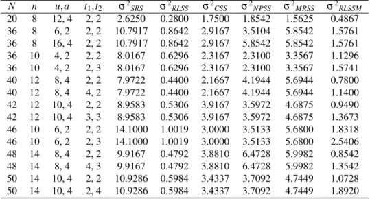
Table (5) shows the values of sampling variances for SRS, RLSS, CSS, NPSS, MRSS and RLSSM obtained from an emperical study for some chosen values ofN andnwith the help of the statistical package R.
Table 5. Variances of the sample mean corresponding to six sampling procedures, namely, SRS, RLSS, CSS, NPSS, MRSS and RLSSM. N n u,a t1,t2 σ2SRS σ2RLSS σ2CSS σ2NPSS σ2MRSS σ2RLSSM 20 8 12, 4 2, 2 2.6250 0.2800 1.7500 1.8542 1.5625 0.4867 36 8 6, 2 2, 2 10.7917 0.8642 2.9167 3.5104 5.8542 1.5761 36 8 16, 4 2, 2 10.7917 0.8642 2.9167 5.8542 5.8542 1.5761 36 10 4, 2 2, 2 8.0167 0.6296 2.3167 2.3100 3.3567 1.1296 36 10 4, 2 2, 3 8.0167 0.6296 2.3167 2.3100 3.3567 1.5741 40 12 8, 4 2, 2 7.9722 0.4400 2.1667 4.1944 5.6944 0.7800 40 12 8, 4 4, 2 7.9722 0.4400 2.1667 4.1944 5.6944 1.1400 42 12 10, 4 2, 2 8.9583 0.5306 3.9167 3.5972 4.6875 0.9490 42 12 10, 4 3, 3 8.9583 0.5306 3.9167 3.5972 4.6875 1.3673 46 10 6, 2 2, 2 14.1000 1.0019 3.0000 3.5133 5.6800 1.8318 46 10 6, 2 2, 3 14.1000 1.0019 3.0000 3.5133 5.6800 2.5406 48 14 8, 4 2, 2 9.9167 0.4792 3.8810 6.4728 5.9982 0.8542 48 14 8, 4 4, 3 9.9167 0.4792 3.8810 6.4728 5.9982 1.3542 50 14 10, 4 2, 2 10.9286 0.5984 3.4337 3.7092 4.7449 1.0728 50 14 10, 4 2, 4 10.9286 0.5984 3.4337 3.7092 4.7449 1.8920
It is obvious from Table (5) that both RLSS and RLSSM outperform the other designs under this type of populations whatever the number of random starts. The RLSS proce-dure has higher efficiency than the proposed design but, as noted earlier, does not offer an unbiased estimator for the sampling variance.
4.3
Auto-correlated Populations
According to Cochran (1946), under this kind of populations it is assumed that two elements yi, yj are positively correlated with a correlation which depends only on the distance ”d =|j−i|” and decreases asd increases. The mean and variance of y0is are supposed to be constant. This type of populations is frequently observed in extensive samplings where the variance within a group of elements increases steadily as the size of the group increases.
E(yi) =µ, Var(yi) =σ2, Cov(yi,yj) =ρdσ2 ∀i6= j (4.11) Under this type of populations, the expected variance of SRS was obtained by Cochran (1946) to be as follows. σ2SRS= ( 1 n− 1 N)σ 2[1− 2 N(N−1) N−1
∑
d=1 (N−d)ρd] (4.12) The expected variance of the multi-start systematic sample mean is given by Gautschi (1957) as: σ2MSSS= k−1 N σ 2[1− 2 N(kt−1) N−1∑
d=1 (N−d)ρd+ 2kt2 n(kt−1) n t−1∑
d=1 (n t −d)ρktd] (4.13)Chang and Huang (2000) gave the expected variance of RLSS in the form:
σ2RLSS=σ 2 N2{k(N−n+r) −2∑d(n−r=1)k−1[(n−r)k−d]ρd+2k2∑n−r−d=1 1(n−r−d)ρdk −2 r(k+1)−1
∑
d=1 [r(k+1)−d]ρd+2(k+1)2 r−1∑
d=1 (r−d)ρd(k+1)} (4.14)The expected variances of CSS and MRSS are given in Huang (2004) by:
σ2CSS= ( 1 n− 1 N)σ 2+2σ2 Nn2 N
∑
t=1 n−1∑
i=0 n−1∑
j>i ρ|(ik+t)−(jk+t)|−2σ 2 N2 N−1∑
d=1 (N−d)ρd (4.15) and σ2MRSS= (1n−N1)σ2+2σ 2 Nn2∑tN=1{k[(n−r−n−r)k−11]∑ (n−r)k−1 i=0 ∑ (n−r)k−1 j>i ρ|(t+j)−(t+i)| +1k∑i(=n−r0 )k−1∑rj=1ρ|(t+i)−[j(k+1)+t+(n−r)k−1]| +∑ri=0∑rj>iρ|[i(k+1)+t+(n−r)k−1]−[j(k+1)+t+(n−r)k−1]|} −2σ 2 N2 N−1∑
d=1 (N−d)ρd (4.16)The expected variance of the NPSS design is obtained by Leu and Tsui (1996) as follows: σ2NPSS= (1n−N1)σ2+Nn22σ2{ a(a−1) u(u−1)∑ N t=1[∑ u−1 i=0 ∑ u−1 (j>iρ|(t+j)−(t+i)|] +au∑Nt=1[∑u−i=01∑ n−a j=1ρ|(t+i)−(jk+t+u−1)|] +∑tN=1[∑in−a=0∑n−aj>i ρ|(ik+t+u−1)−(jk+t+u−1)|]}
− 2 N2σ 2N−1
∑
d=1 (N−d)ρd (4.17)The expected variance under the RLSSM design is given in the next theorem.
Theorem6: The expected variance of the mean of the RLSSM design is obtained in the following form: σ2RLSSM= σ 2 N2{k(N−n+r)− 2(k−1) t1k−1 ∑ (n−r)k−1 d=1 [(n−r)k−d]ρd+ 2t22k(k+1)2 [t2(k+1)−1] ×∑ r t2−1 d=1( r t2−d)ρdt2(k+1)+ 2t12k2(k−1) t1k−1 ∑ n−r t1 −1 d=1 ( n−r t1 −d)ρdt1k − 2k [t2(k+1)−1] r(k+1)−1
∑
d=1 [r(k+1)−d]ρd} (4.18)Proof: LetEM[Var(y¯RLSSM)] =ξ[Var(y¯RLSSM)] =σRLSSM2 , then we have the following;
σ2RLSSM= N12{ (n−r)2k2(k−1) t1k−1 ξ[ 1 t1k∑ t1k i=1(y¯1i−Y¯1)2] + r2(k+1)2k [t2(k+1)−1] ×ξ[t2(k1+1)∑ti2(=k1+1)(y¯2i−Y¯2)2]}. LetI= (n−r)2k2tk−1 1k−1ξ[ 1 t1k∑ t1k i=1(y¯1i−Y¯1)2] andII=r2(k+1)2[t2(k+k1)−1]ξ[t2(k1+1)∑it=2(1k+1)(y¯2i−Y¯2)2]. Working onIgives; I= (n−r)2k2(tk−1 1k−1) t1σ2 n−r(1− 1 t1k){1− 2 (n−r)k(t1k−1)∑ (n−r)k−1 d=1 [(n−r)k−d]ρd + 2t12k (n−r)(t1k−1)∑ (n−r) t1 −1 d=1 [ n−r t1 −d]ρdt1k} = (n−r)k(k−1)σ2{1−(n−r)k2(t 1k−1)∑ (n−r)k−1 d=1 [(n−r)k−d]ρd+ 2t12k (n−r)(t1k−1) ×∑ n−r t1 −1 d=1 [ n−r t1 −d]ρdt1k}
II=r2(k+1)2[t k 2(k+1)−1]. t2σ2 r (1− 1 t2(k+1)){1− 2 r(k+1)[t2(k+1)−1]∑ r(k+1)−1 d=1 [r(k+1)−d]ρd + 2t22(k+1) r[t2(k+1)−1]∑ r t2−1 d=1[ r t2−d]ρdt1(k+1)} =rk(k+1)σ2{1−r(k+1)[(t2(2k+1)−1]∑rd(=k+11)−1[r(k+1)−d]ρd+ 2t 2 2(k+1) r[t2(k+1)−1] ×∑ r t2−1 d=1 [ r t2−d]ρdt1(k+1)}
Thus,σ2RLSSM= N12[I+II] = (4.18). Hence the theorem follows.
It can be easily verified that whent1=t2=1, expression (4.18) reduces to (4.14). In other words, the expected variance of RLSSM is reduced to that of RLSS when only one random start is selected. Additionaly, if there is no remainder term,r=0, the proposed design is equivalent to the multi-start systematic sampling design and (4.18) reduces to (4.13).
Looking at formulas (4.12) through (4.18) shows the difficulty in obtaining a general result about the relative efficiency of the considered sampling designs. However, per-formance comparisons can be carried out empirically for three types of correlograms considered by Cochran (1946), which are
i. Linear correlogram:ρd=1−d/L ; L≥N−1 ii. Exponential correlogram:ρd=e−λd
iii. Hyperbolic correlogram:ρd=tanh(d−3/5)
where correlogram is the curve, or the function produced by ploting the set of corre-lationsρd for pairs of units that aredunits apart againstd.
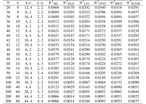
Taking L=N and λ =1, the numerical values of the expected variance of the sample
mean under each of SRS, RLSS, CSS, NPSS, MRSS and RLSSM are obtained, using R package for statistical computing, for the three types of correlograms as in Tables (6), (7) and(8), respectively.
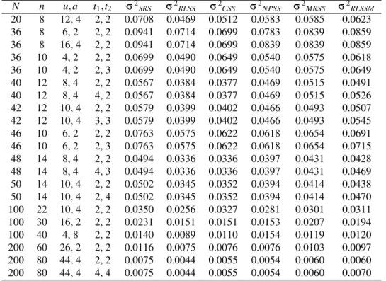
Clearly, the numerical results in Tables (6), (7) and (8), show that the proposed sam-pling procedure is better than SRS for the three different types of correlogram regardless the number of random starts. Compared with RLSS procedure, the suggested sampling design has higher expected variance in all cases. However, the propsed design still has the merit over RLSS by handling the two main statistical issues of LSS simultaneously. On the other hand, the suggested sampling procedure is more efficient than CSS in most cases, espcially for large population and sample sizes, for populations with linear correl-ogram.
Table 6. The Expected variances corresponding to six sampling procedures, namely, SRS, RLSS, CSS, NPSS, MRSS and RLSSM for populations exhibt a linear correlogram(ρd=1−(d/N)).
N n u,a t1,t2 σ2SRS σ2RLSS σ2CSS σ2NPSS σ2MRSS σ2RLSSM 20 8 12, 4 2, 2 0.0263 0.0050 0.0175 0.0185 0.0156 0.0087 36 8 6, 2 2, 2 0.0333 0.0051 0.0090 0.0108 0.0181 0.0094 36 8 16, 4 2, 2 0.0333 0.0051 0.0090 0.0181 0.0181 0.0094 36 10 4, 2 2, 2 0.0247 0.0033 0.0072 0.0071 0.0104 0.0058 36 10 4, 2 2, 3 0.0247 0.0033 0.0072 0.0071 0.0104 0.