SUBQUADRATIC-TIME FACTORING OF POLYNOMIALS OVER FINITE FIELDS

Volume 67, Number 223, July 1998, Pages 1179–1197 S 0025-5718(98)00944-2

SUBQUADRATIC-TIME FACTORING OF POLYNOMIALS OVER FINITE FIELDS

ERICH KALTOFEN AND VICTOR SHOUP

Abstract. _{New probabilistic algorithms are presented for factoring univariate} polynomials over finite fields. The algorithms factor a polynomial of degree

nover a finite field of constant cardinality in time O(n1.815). Previous al-gorithms required time Θ(n2+o(1)). The new algorithms rely on fast matrix multiplication techniques. More generally, to factor a polynomial of degree

nover the finite fieldFq withqelements, the algorithms use O(n1.815logq) arithmetic operations inFq.

The new “baby step/giant step” techniques used in our algorithms also yield new fast practical algorithms at super-quadratic asymptotic running time, and subquadratic-time methods for manipulating normal bases of finite fields.

1. Introduction

In this paper, we present a new probabilistic approach for factoring univariate polynomials over finite fields. The resulting algorithms factor a polynomial of degree

nover a finite fieldF_q whose cardinalityq is constant in timeO(n1.815_{). The best}

previous algorithms required time Θ(n2+o(1)_).

This running-time bound relies on fast matrix multiplication algorithms. Letω

be an exponent of matrix multiplication; that is,ωis chosen so that we can multiply twon×nmatrices usingO(nω_{) arithmetic operations (we assume that 2< ω≤3).} Using the result of Coppersmith and Winograd [11], we can takeω <2.375477.

More generally, we prove the following:

Theorem 1. For any0≤β≤1, there exists a probabilistic algorithm for factoring a univariate polynomial of degree n over a finite field F_q that uses an expected number of

O(n(ω+1)/2+(1−β)(ω−1)/2+n1+β+o(1)logq) Received by the editor October 12, 1995 and, in revised form, March 29, 1996. 1991Mathematics Subject Classification. Primary 12E20, 13P05, 68Q40.

Key words and phrases. Factoring, polynomials, finite fields, randomized algorithms, normal bases.

This material is based on work supported in part by the National Science Foundation under Grant No. CCR-9319776 (first author) and by an Alexander von Humboldt Research Fellowship (second author).

A major part of the work was performed while the first author was at Rensselaer Polytechnic Institute, Department of Computer Science, in Troy, New York and while the second author was at the Universit¨at des Saarlandes, FB 14–Informatik, in Saarbr¨ucken, Germany.

A preliminary version of this paper appears in the Proc. 27th Annual ACM Symp. Theory of Computing, ACM Press, pp. 398–406 (1995).

c

1998 American Mathematical Society

arithmetic operations inFq. In particular, choosing ω <2.375477and minimizing the exponent of n, we getO(n1.815logq)operations inF_q.

Relation to Previous Work. The first random polynomial-time algorithm for this problem is due to Berlekamp [4]. Berlekamp’s algorithm reduces the problem to that of finding elements in the null space of ann×nmatrix overFq. Using standard techniques from linear algebra, Berlekamp’s algorithm can be implemented so as to use an expected number of O(nω+n1+o(1)logq) operations inFq. Note that the algorithm by Rabin [31] has an inferior running time, but Rabin completes the mathematical justification for the expected running time of the probabilistic Berlekamp method.

A very different algorithm is described by Cantor and Zassenhaus [9] (see also Ben-Or [3], especially for the case where the characteristic is 2). Starting with a square-free polynomial, that algorithm first separates the irreducible factors of dis-tinct degree (disdis-tinct-degree factorization), and then completely factors each of the resulting factors (equal-degree factorization). The Cantor/Zassenhaus algorithm can be implemented so as to use an expected number ofO(n2+o(1)logq) operations inFq.

Von zur Gathen and Shoup [17] developed new algorithmic techniques that es-sentially allow one to implement the Cantor/Zassenhaus algorithm so that it uses an expected number of O(n2+o(1) _+n1+o(1)_{logq) operations in Fq. Their}

tech-niques allow one to solve the special problem of equal-degree factorization using an expected number ofO(n(ω+1)/2+o(1)_+n1+o(1)_{logq) operations inF}

q.

Niederreiter [28] developed an alternate approach to factoring polynomials over finite fields. However, from a complexity point of view this method is closely related to Berlekamp’s original algorithm (Fleischmann [15] Niederreiter and G¨ottfert [29]). Kaltofen and Lobo [20] adapted the linear system solver of Wiedemann [36] to Berlekamp’s algorithm. Utilizing techniques from von zur Gathen and Shoup, they show how their Black Box Berlekamp algorithm can be implemented so as to use an expected number ofO(n2+o(1)+n1+o(1)logq) inF_q.

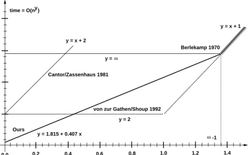
Notice that atβ = 0, the running-time of our algorithm matches that of Ber-lekamp’s, and atβ= 1 it matches that of Cantor/Zassenhaus, so that in some sense it interpolates between these two algorithms.

When logqis not too large in relation ton, then our new algorithm is asymptot-ically faster than previous algorithms. This is certainly clear ifqis a constant and

ω <3. Also, forω <2.375477, as nandq tend to infinity with logq=O(n0.454_),

our new algorithm usesO(n2−Ω(1)) operations inF_q, whereas the best previous algo-rithms require Θ(n2+o(1)) operations. Figure 1 plots the running times of selected algorithms in dependence of both n and logq when a fast matrix multiplication algorithm is used. The method by von zur Gathen and Shoup to-date remains the champion when logq= Ω(n0.454_{) and simultaneously logq=O(n}1.375477_{). At}

larger fields the term nlogq in the Berlekamp algorithm dominates all running times.

Overview. Our Theorem 1 is proved using the Cantor/Zassenhaus strategy. The main technical contribution here is a subquadratic distinct-degree factorization algorithm, which is based on a “baby step/giant step” strategy. Our Fast Cantor/Zassenhaus algorithm is described in§2.

We also show how to modify the Black Box Berlekamp algorithm, using a very similar baby step/giant step technique, to get a subquadratic-time algorithm as

x 1.8 2.0 2.2 2.4 2.6 0.0 0.2 0.4 0.6 0.8 1.0 1.2 1.4 Ours

von zur Gathen/Shoup 1992

Berlekamp 1970 Cantor/Zassenhaus 1981 y log(q) = O(n )x time = O(n )y ω y = 2 y = y = x + 2 y = x + 1 y = 1.815 + 0.407 x _ω -1

Figure 1. _{Running time comparisons for variable field cardinality}

well. This algorithm is described in§3. Interestingly, our techniques for the Black Box Berlekamp algorithm lead to subquadratic algorithms for finding a normal element in a finite field and for converting to and from normal coordinates. We present those algorithms in §4.

At the heart of our algorithms is the following problem. Given polynomialsf,

g, andhin F_q[x] of degree bounded by n, compute g(h) modf ∈F_q[x]. Recently, this so-calledmodular polynomial compositionproblem has arisen in many contexts (von zur Gathen and Shoup [17], Shoup [34]). The algorithm of Brent and Kung [6] solves this problem usingO(n(ω+1)/2) operations inFq.

Any improvement in the complexity of this problem would yield an improve-ment in the complexity of factoring. Indeed, if this problem could be solved using

O(n1+o(1)) operations inFq, then our Fast Cantor/Zassenhaus algorithm could be implemented so as to useO(n1.5+o(1)+n1+o(1)logq) operations inF_q.

Our algorithms rely on fast multiplication of matrices, indeed of n1/2×n1/2

matrices, and therefore are not particularly practical. Interestingly, however, the techniques themselves can be adapted so as to give a quite practical factoring algorithm that uses

O(n2.5+n1+o(1)logq) operations in F_q and space for O(n1.5_{) elements inF}

q, where the implied “big-O” constants are quite reasonable. From practical experience, we have found that whenq is a large prime, this new algorithm allows much larger polynomials to be factored using a reasonable amount of space and time than was previously possible using other algorithms. This is briefly discussed in§5; a more complete discussion, including a description of an implementation of this algorithm as well as the results of empirical tests, is given in Shoup [35].

To attain a subquadratic running time, our algorithms rely on randomization. Even if we restrict ourselves to the field F2, the asymptotically fastest known

de-terministic algorithm (Shoup [33]) runs in timeO(n2+o(1)_{), and it remains an open}

problem to find a subquadratic deterministic algorithm.

2. The fast Cantor/Zassenhaus algorithm

Like the original Cantor/Zassenhaus algorithm, our algorithm splits the problem of factoring into three sub-problems:

Square-free factorization: The input is a polynomial f ∈F_q[x] of degree n. The output isf1, . . . , fn∈Fq[x] such that

f =f1·f22· · · · ·fnn.

Distinct-degree factorization: The input is a square-free polynomial f ∈

Fq[x] of degreen. The output isf[1], . . . , f[n]∈Fq[x] such that for 1≤d≤n,

f[d] _{is the product of the monic irreducible factors off of degreed.}

Equal-degree factorization: The input is a polynomial f ∈ Fq[x] of degree

n and an integer d such that f is the product of distinct monic irreducible polynomials, each of degree d. The output is the set of irreducible factors off.

The factoring algorithm proceeds in three stages as follows. In the first stage, the input polynomial is fed into a square-free factorizer. In the second stage, the non-trivial outputs from the first stage are fed into distinct-degree factorizers. In the last stage, the non-trivial outputs from the second stage are fed into equal-degree factorizers.

The square-free factorization problem can be solved on degree n inputs using

O(n1+o(1)_{+nlogq) operations inF}

q, using the algorithm of Yun (see Knuth [23]). The equal-degree factorization problem can be solved on degree ninputs with the probabilistic algorithm of von zur Gathen and Shoup [17] using an expected number of

O(n(ω+1)/2+o(1)+n1+o(1)logq),

or

O(n1.688+n1+o(1)logq) operations inF_q.

We shall now present a family of (deterministic) algorithms for the distinct-degree factorization problem, parameterized byβ with 0≤β ≤1, that uses

O(n(ω+1)/2+(1−β)(ω−1)/2+n1+β+o(1)logq)

operations inF_q. For any choice ofβ, this dominates the time required for square-free factorization and equal-degree factorization, establishing Theorem 1.

Our distinct-degree factorization algorithm uses a “baby step/giant step” strat-egy that exploits the following fact.

Lemma 1. For nonnegative integers i and j, the polynomial xqi _−xqj _{∈ F} q[x] is

divisible by precisely those irreducible polynomials inFq[x]whose degree dividesi−j. Proof. Assume without loss of generality thati≥j. Thenxqi_−xqj _{= (x}qi−j_−x)qj_, and the result follows at once from the factorization ofxqk−x, which consists of

all irreducible factors whose degree is a divisor ofk(see Lidl and Niederreiter [24], Theorem 3.20).

We first present a high-level description of our distinct-degree factorization al-gorithm. The details of how each step is to be implemented are deferred until later.

Algorithm D. This algorithm takes as input a square-free polynomial f ∈ F_q[x] of degree n. The output is f[1]_{, . . . , f}[n] _{∈ F}

q[x] such that for 1≤ d≤ n, f[d] is the product of the monic irreducible factors of f of degree d. The algorithm is parameterized by a constantβ, with 0≤β ≤1.

Step D1 (compute baby steps): Let l = dnβ_{e. For 0 ≤ i ≤ l, compute}

h_i=xqi modf ∈F_q[x].

Step D2 (compute giant steps): Letm=dn/2le. For 1≤j ≤m, compute

H_j =xqlj _{modf ∈F} q[x].

Step D3 (compute interval polynomials): For 1≤j≤m, compute

I_j = Y

0≤i<l

(H_j−h_i) modf ∈Fq[x].

Note that by Lemma 1, the polynomial I_j is divisible by those irreducible factors off whose degree divides an integerkwith (j−1)l < k ≤jl.

Step D4 (compute coarse DDF): In this step, we compute polynomials

F1, . . . , Fm, whereFj =f[(j−1)l+1]f[(j−1)l+2]· · ·f[jl]. This is done as follows.

f∗←f;

forj←1 tomdo

{F_j ←gcd(f∗, I_j);f∗←f∗/F_j }

Step D5 (compute fine DDF): In this step, we compute the output polyno-mialsf[1]_{, . . . , f}[n]_{. First, initializef}[1]_{, . . . , f}[n]_{to 1. Then do the following.}

forj←1 tomdo {g←F_j; fori←l−1 down to 0 do {f[lj−i]_{←gcd(g, H} j−hi);g←g/f[lj−i]} } iff∗6= 1 thenf[deg(f∗)]←f∗;

The correctness of this algorithm is clear from the comments contained therein. Before establishing the running-time bound in Theorem 1, we begin with the following slightly weaker, but simpler, result.

Theorem 2. Algorithm D can be implemented so as to use O(n(ω+1)/2+1−β+n1+β+o(1)logq)

operations inF_q. In particular, choosingω <2.375477and minimizing the exponent of n, we getO(n1.844logq)operations inF_q.

The proof of Theorem 2 is based on the observation that for any positive integer

r, if we are given h=xqr _{modf ∈Fq[x], then for anyg∈Fq[x], we can compute}

gqr_{modf as g(h) modf ∈ F}

q[x]. To solve this so-called “modular composition” problem, we use the following result.

Lemma 2. Given a polynomial f ∈ K[x] of degree n over an arbitrary field K, and polynomials g, h∈K[x] of degree less than n, we can compute the polynomial g(h) modf ∈K[x] usingO(n(ω+1)/2_{)arithmetic operations inK.}

Proof. This is essentially Algorithm 2.1 in Brent and Kung [6]. We now prove Theorem 2.

Step D1 is performed by iterating the standard repeated-squaring algorithm l

times. This takesO(n1+β+o(1)_{logq) operations inF}

q.

Step D2 is performed by setting H1 = hl, and then iterating the algorithm of Lemma 2, computing each H_j as H_j−1(H1) modf ∈ Fq[x]. This takes

O(n(ω+1)/2+1−β) operations inF_q.

Step D3 is performed as follows. LetRbe the ringFq[x]/(f). We first compute the coefficients of the polynomialH(Y)∈R[Y] of degreel, where

H(Y) = Y

0≤i<l

(Y −(h_imodf)).

Then we evaluateH(Y) at thempoints

(H1modf), . . . ,(Hmmodf)∈R.

Using fast algorithms for multiplication of polynomials in R[Y] (Cantor and Kaltofen [8]) Step D3 can be implemented so as to use O(n1+β+o(1)+n2−β+o(1)) operations inF_q (Aho et al. [1]).

In Step D4, we need to compute O(m) GCD’s and divisions, requiring

O(n2−β+o(1)_{) operations inFq.}

To implement Step D5 efficiently, we first reduce eachh_i modulo eachF_j. Re-ducing one h_i modulo each F_j takes O(n1+o(1)_{) operations in F}

q, using standard “Chinese remaindering” techniques (Aho et al. [1]). Thus, reducing all of theh_i’s modulo all of theF_j’s takes justO(n1+β+o(1)_{) operations inF}

q. Also, we compute

H_jmodF_j for each F_j. This takes O(n2−β+o(1)_{) operations in F}

q. With these pre-computations, the total cost of computing the GCD’s and divisions in the inner loop amounts toO(n1+β+o(1)_{) operations inF}

q. Thus the total cost of Step D5 is

O(n1+β+o(1)_+n2−β+o(1)_{) operations inF}

q. That proves Theorem 2.

We now show how to modify the implementation of Step D2 to obtain the slightly better running-time bound of Theorem 1.

Theorem 3. Algorithm D can be implemented so as to use O(n(ω+1)/2+(1−β)(ω−1)/2+n1+β+o(1)logq)

operations inF_q. In particular, choosingω <2.375477and minimizing the exponent of n, we getO(n1.815logq)operations inF_q.

To prove this theorem, it will suffice to show that we can compute the polynomi-alsH1, . . . , Hm in Step D2 usingO(n(ω+1)/2+(1−β)(ω−1)/2) operations inFq. This is an immediate consequence of the following two lemmas.

Lemma 3. Given a polynomialf ∈K[x]of degreenover an arbitrary fieldK, and polynomials g1, . . . , gk, h ∈ K[x] of degree less than n, where k = O(n), we can

compute

using

O(n(ω+1)/2k(ω−1)/2)

arithmetic operations in K.

Proof. Settingt=d√nke, we decompose each of the input polynomialsg1, . . . , gk as

g_i= X

0≤j<n/t

g_i,jyj, y=xt_, (1)

where the g_i,j’s are polynomials of degree less thant. We first compute the poly-nomials h(i) _{= h}i_{modf for 0 ≤ i ≤ t. Next, we compute all of the} polynomi-als g_i,j(h) modf by computing the following product of an n×t matrix and a

t×(kdn/te) matrix: h ~h(0) _{. . . ~h}(t−1) i_·~g 1,0 . . . ~g1,dn/te−1 . . . ~gk,0 . . . ~gk,dn/te−1 .

Here, we use the notation~· to denote the column vector consisting of the coefficients of a polynomial. This computation is done by performingO(pn/k) multiplications oft×tmatrices. Finally, we compute for 1≤i≤kthe polynomialg_i(h) modf(x)∈ K[x] by substituting the polynomial h(t) _{fory in the formula (1), and performing}

a Horner evaluation scheme. This is done by iteratively performing dn/te − 1 polynomial multiplications modf and O(n/t) polynomial additions.

It is easily seen that the dominant cost is again the matrix multiplication step, which can be carried out using the stated number of operations.

We remark that when k = 1, the algorithm in the above proof is the same as Brent and Kung’s modular composition algorithm.

Lemma 4. Let f ∈F_q[x] be a polynomial of degreen. Suppose that we are given xqr _{modf ∈F}

q[x]. Then we can compute

xqr modf, xq2r modf, . . . , xqkr modf ∈F_q[x], wherek=O(n), using

O(n(ω+1)/2k(ω−1)/2)

operations in F_q.

Proof. For i ≥ 1, let G_i = xqir _{modf ∈ F}

q[x]. Assume we have computed

G1, . . . , Gm. Then we can compute Gm+1, . . . , G2m by computing G1(Gm) mod

f, . . . , G_m(G_m) modf using the algorithm in the previous lemma.

So to computeG1, . . . , Gk givenG1, we simply repeat the above “doubling” step O(logk) times. The stated running-time estimate then follows easily.

3. The Fast Black Box Berlekamp algorithm

In Kaltofen and Lobo [20], a version of Berlekamp’s factoring algorithm was given based on Wiedemann’s [36] sparse linear system solver. In this section, we show how to modify that algorithm to obtain a probabilistic, subquadratic-time algorithm.

We split this section into two parts. In §3.1, we review the ideas behind the Black Box Berlekamp algorithm, presenting a high-level description of that algo-rithm. Then in§3.2, we describe a subquadratic-time implementation, first proving

a running time bound of O(n1.880+n1.808logq) operations inFq. We then modify this method to obtain the boundO(n1.852+n1.763logq). With yet a bit more work, we show how to obtain the boundO(n1.815_logq).

3.1. The Black Box Berlekamp Algorithm. We first recall the main ideas behind the Black Box Berlekamp algorithm. Suppose the coefficient field Fq has characteristicp. Let f ∈F_q[x] be a monic square-free polynomial of degreento be factored. Assume that the factorization off into irreducibles is

f =f1· · ·fr.

For 1≤i≤r, let d_i = deg(f_i), and letpei _{be the highest power ofpthat divides}

d_i. Furthermore, lete= max{e_i: 1≤i≤r}.

Now consider the q-th power map σ:α7→αq _{for α∈F}

q[x]/(f). Let φ∈Fq[λ] be the minimum polynomial of σover F_q, i.e., φ is the monic polynomial of least degree such thatφ(σ) = 0. The polynomialφ can easily be described in terms of the degrees of the irreducible factors of f, as follows. By the Chinese remainder theorem we have theFq-algebra isomorphism

Fq[x]/(f)∼=Fq[x]/(f1)⊕ · · · ⊕Fq[x]/(fr).

For 1 ≤ i ≤ r, let σ_i be the q-th power map on Fq[x]/(f_i), and let φ_i ∈ Fq[λ] be its minimum polynomial. From the basic theory of finite fields, we know that

φ_i=λdi−_{1. Moreover, by the Chinese remainder theorem,}

φ= lcm{φ1, . . . , φr}= lcm{λd1−1, . . . , λdr−1}.

Now consider the polynomial µ(λ) =φ(λ)/(λ−1), and the imageI_i ⊂F_q[x]/(f_i) ofµ(σ_i). Since (σ_i−1)(α) =αq−α= 0 for allα∈I_i, it follows thatI_i⊂F_q. It is easily seen that λ−1 dividesλdi−_{1 exactly to the power p}ei_{, which implies that}

I_i=F_q ife_i =e, and I_i ={0} ife_i < e(see Kaltofen and Lobo [20], §3, for more details).

These considerations motivate the following recursive algorithm. The details of how each step is to be implemented are deferred until later.

Algorithm B. The algorithm takes as input a monic square-free polynomialf ∈

Fq[x] of degreen, and produces as output the set of irreducible factors off.

Step B1 (compute minimum polynomial): Probabilistically compute a polynomialφ∗∈F_q[λ] that with probability at least 1/2 is equal toφ, the min-imum polynomial of the q-th power mapσ onF_q[x]/(f), and that otherwise dividesφ.

Step B2 (evaluate polynomial): If φ∗(λ) =λn_{−1, then halt, as f is then} certified to be irreducible. Ifλ−1 does not divideφ∗(λ), go back to Step B1, as thenφ∗is clearly erroneous. Otherwise, setµ∗(λ) =φ∗(λ)/(λ−1), choose a randomα∈F_q[x]/(f), and compute

α∗= (µ∗(σ))(α)∈F_q[x]/(f).

Step B3 (split): Letα∗= (gmodf). Computeh1= gcd(g, f) andh2=f /h1.

Ifφ∗ =φthen the degrees of all irreducible factors of h2 are divisible by pe

and the residues ofh2modulo these factors are random elements in Fq\ {0}. Computeh∗∈F_q[x]/(h2) as h∗= ( g(q−1)/2modh2 ifp >2, P_k−1 j=0g2 j modh2 ifq= 2k.

Recursively factorh1,h∗2= gcd(1 +h∗modh2, h2) andh2/h∗2.

Before going into the details of each step, we first calculate a bound on the recursion depth of this algorithm.

Lemma 5. The expected value of the recursion depth of Algorithm B is O(dlog_pnelogr), wherer is the number of irreducible factors off.

Proof. Consider one invocation of the algorithm and recall the notation preceding the algorithm. Each factor f_i with e_i = e will be separated from the factorsf_j

withe_j < ein Step B3 with probability bounded away from 0 by a constant. Iff

has several factors with e_i=e, then each pair of such factors will be separated in Step B3 with probability bounded away from 0 by a constant. These statements follow easily from the fact thatφ∗ is correctly computed with probability 1/2, and from the discussion preceding the algorithm.

Using a standard argument (see, for example, Lemma 4.1 in von zur Gathen and Shoup [17], at an expected depth of O(logr), all irreducible factorsf_i withe_i =e

will be isolated, and the only reducible factors remaining will havee_i< e.

It follows that at an expected depth ofO(dlog_pnelogr), all irreducible factors off will be isolated.

Next, we discuss the problem of computingφ∗in Step B1. Following Wiedemann [36], this is done as follows. We choose randomα ∈ F_q[x]/(f) and a random Fq -linear mapu:F_q[x]/(f)→F_q, and compute the minimum polynomial of the linearly generated sequence {a_i :a_i =u(σi(α)) andi ≥0}. Using an asymptotically fast version of the Berlekamp-Massey algorithm (Massey [27], Dornstetter [12]), given the first 2n terms of the sequence {a_i : i ≥ 0}, we can determine the minimum polynomial φ_α,u ∈ F_q[λ] of this sequence using O(n1+o(1)_{) operations in F}

q. In general,φ_α,udividesφ, but the probability thatφ_α,u=φ(for randomα,u) may be less than 1/2, and indeed not even bounded away from 0 by a constant. To increase this probability, we repeat the above procedure some number ρ(n, q) times, each time choosing a newαand a newuat random, thus obtaining polynomialsφ_αi,ui, where 1≤i≤ρ(n, q). Then we compute

φ∗= lcm{φ_αi,ui : 1≤i≤ρ(n, q)}.

The valueρ(n, q) can be chosen as indicated in the next lemma.

Lemma 6. Let ρ(n, q)be defined as follows. If q≥4n, then ρ(n, q) = 1. Other-wise, ρ(n, q) =        6 if q= 2, 4 if q= 3, 3 if 4≤q≤9, 2 if q≥11. Then the probability thatφ∗=φis at least1/2.

Proof. If q ≥ 4n, then the result follows by the analysis of Kaltofen and Pan [21]. Otherwise we argue along the same lines as Wiedemann [36, §VI]. Suppose

φ =ψη₁1· · ·ψηs

s is the factorization ofφ into irreducibles. Suppose α ∈Fq[x]/(f) and u: F_q[x]/(f) → Fq are chosen at random. As above, let φ_α ∈ F_q[λ] be the minimum polynomial of the sequence{σi(α) :i≥0}and letφ_α,ube the minimum polynomial of the sequence{u(σi(α)) :i≥0}.

Claim. For any singlej with 1≤j ≤s, the probability that ψ_jηj does not divide

φ_α,u is no more than

(2/q−1/q2)δ whereδ= deg(ψ_j).

We prove this claim by using a fact established by Wiedemann. He shows that there exists a surjective Fq-linear map L: V → W depending on α, where V is the linear space ofF_q-linear maps fromF_q[x]/(f) toFq and W is the linear space of polynomials of degree less than deg(φ_α), such that for any u ∈ V we have

φ_α,u = φ_α/gcd(φ_α,L(u)). Suppose now that ψη_jj divides φ_α. Then ψ_jηj divides

φ_α,u if ψ_j does not divide L(u), which for a random u is a random polynomial overF_q of degree less than deg(φ_α). Clearly, of allqdeg(φα)_{such polynomials only} qdeg(φα)−δ _{are divisible byψ}

j, so the probability that ψj does not divideL(u) is 1−1/qδ. Furthermore, by considering the rational canonical form of the linear transformσwe can show the existence of an elementα0 such thatφα0 =φ. As L

is surjective, there also must exist au0 such thatφα0,u0 =φα0 =φ. By switching

the rˆoles ofuandα, as Wiedemann does in the proof of his Proposition 4, we can obtain that the probability thatψ_jηj dividesφ_α,u0 is 1−1/qδ_{. Thus, the probability} thatψ_jηj dividesφ_α is no less.

Therefore, the probability that ψη_jj does not divide φ_α,u is no less than 1− (1−1/qδ₎2_{= 2/q}δ_−1/q2δ_{. The claim then follows from the inequality 2c}δ_−c2δ_≤ (2c−c2₎δ_{, which holds for all real numbers c with 0 < c ≤ 1/2 and all integers}

δ≥1.

From this claim, one sees that if this procedure is repeatedk = ρ(n, q) times, and we compute φ∗ as the polynomial least common multiple of all of theφ_αi,ui’s, then the probability that ψ_jηj does not divideφ∗ is at most (2/q−1/q2₎kdeg(ψj)_.

Since the factorization ofxql_{−xincludes each irreducible polynomial of degree}

l, the number of irreducibles of degree l is at most ql_{/l. Hence summing over all} irreducible polynomials dividingφ, as well as all those irreducible polynomialsnot

dividingφ, we get an upper bound on the probability that φ∗6=φof

X l≥1 ql l (2/q−1/q 2 )k l =−log(1−q(2/q−1/q2)k).

The lemma then follows from a simple numerical calculation.

For sufficiently largeqit is possible to improve the expected recursion depth of Algorithm 1 to O(log_pn+ logr) as follows. First, we make the probability that

φ∗6=φin Step B1 smaller than 1/q by computing the least common multiple ofρ0

many polynomialsφ_αi,ui, where

ρ0(n, q) =            6 ifq= 2, 5 ifq= 3, 4 ifq= 4,5, 3 ifq≥7, 2 ifq >4n2_.

The values for ρ0 follow as in the proof of Lemma 6. Suppose now that φ∗ =φ. Then the probability that allr_eirreducible factorsf_ioff withe_i =eare separated from the remaining factors in a single gcd in Step B3 is equal to the probability that

Overall, we succeed to separate thef_iwithe_i=efrom the rest in a single try with probability≥(1−1/q) (1−1/q)re_.

Let r_η be the number of irreducible factors f_j of f with e_j = η. Then with probability no less than

e Y η=0 1−1 q 1+rη ≥ 1−1 q e+r+1 ≥ 1 4 (e+r+1)/q

the factors with e_j =η are split off for all η by a recursion of depth e+ 1. Now suppose that for a constantc >0 we have

q≥c(blog_pnc+r+ 1).

Then the probability that all pairsf_iandf_jwithe_i6=e_j are separated at recursion depth O(log_pn) is bounded away from 0 by a constant (namely 4−1/c_{). It is then} easy to show that the expected depth isO(log_pn+ logr). We note that for constant

q, however, the expected recursion depth can be Θ((logn)2). 3.2. A Subquadratic-Time Implementation.

Theorem 4. For any constantβ with0≤β ≤1, Algorithm B can be implemented so as to use an expected number of

O(n(ω+1)/2+(3−ω)|β−1/2|+o(1)+n(ω+1)/2+1−β+o(1)+n1+β+o(1)logq) (2)

operations inF_q. In particular, choosingω <2.375477and minimizing the exponent of n, we getO(n1.880+n1.808logq)operations inFq.

Remark 1. The first term in (2) is dominated by the second exactly when β <

(ω−5)/(2(ω−4)), and thus at least whenβ <3/4.

To prove Theorem 4, we first show that one invocation of Algorithm B, not counting the recursive calls, can be implemented so as to satisfy the bound in Theorem 4. By Lemma 5, multiplying this by O((logn)2) gives a bound on the total cost of the algorithm, and thus the theorem will follow.

The cost of Step B3 is O(n1+o(1)_{logq) operations in F}

q, and the cost of the Berlekamp-Massey algorithm in Step B1 is O(n1+o(1)) operations in F_q. So to prove our result, we have to solve the following two types of problems within the stated time bounds.

automorphism projection: Given α ∈ F_q[x]/(f), u: F_q[x]/(f) → F_q, and a positive integerk=O(n), computeu(σi_(α))∈F

q for alliwith 0≤i < k.

automorphism evaluation: Given α∈F_q[x]/(f) and a polynomial µ∈F_q[λ] of degree less thank, where k=O(n), compute (µ(σ))(α)∈F_q[x]/(f). We first claim that these two problems are computationally equivalent, in a very strong sense. Consider the n×kmatrixA whose columns consist of the co-ordinates with respect to the natural power basis 1, x, x2, . . . , xn−1 for Fq[x]/(f) of α, σ(α), . . . , σk−1_{(α). Then the automorphism projection problem consists of}

multiplying A on the left by a row vector (u0, . . . , un−1)∈ F_q1×n. The

automor-phism evaluation problem consists of multiplyingAon the right by a column vector (µ0, . . . , µk−1)T∈F_qk×1. Thus these two problems are merely the transpose of each

other, and by the so-calledtransposition principlea straight-line program of lengthl

for one can be quickly converted (in timeO(l)) into a straightline program of length

input variables {u_i} (respectively,{µ_i}). It should be noted that this observation applies to the Wiedemann algorithm in general. For example, in Algorithm 1 in Wiedemann [36] step 4 and step 6 are computationally equivalent within a constant factor. The discovery of the transposition principle goes back to the Ph.D. thesis of Fiduccia [14], Theorem 2 for multiplications (see also Fiduccia [13], Theorem 4) and Theorem 5 for additions and subtractions. The additive version with a similar proof is rediscovered in (Kaminski et al. [22]). Furthermore, we remark that the transposition principle is a direct consequence of the so-called reverse mode in au-tomatic differentiation, see Canny et al. [7]; for reverse mode see also Ostrowski et al. [30], Linnainmaa [25], Baur and Strassen [2], and Griewank [19].

Thus, to prove our theorem, it will suffice to prove the required bound for just one of these problems. We prove it for the automorphism evaluation problem. The following algorithm for automorphism evaluation is based on the same “baby step/giant step” strategy used in Brent and Kung’s modular composition algorithm.

Algorithm AE. This algorithm takes as input an elementα ∈F_q[x]/(f), where

f ∈ F_q[x] is of degree n, and a polynomialµ ∈F_q[λ] of degree less thank, where

k =O(n). The output is (µ(σ))(α) ∈Fq[x]/(f). The algorithm is parameterized by a constantβ, with 0≤β ≤1.

We sett=dnβ_{eandm=dk/te, and we write µas}

µ= X

0≤j<m

µ_j(λ)λtj,

where eachµ_j∈Fq[λ] has degree less thant. Then we have

(µ(σ))(α) = X

0≤j<m

σtj( (µ_j(σ))(α) ).

The algorithm proceeds as follows.

Step AE1: Compute σi_{(α) ∈ F}

q[x], for all i with 0 ≤ i < t, by iterating a repeated squaring algorithm.

Step AE2: Using the values computed in Step AE1, we next compute (µ_j(σ))(α)∈F_q[x] for allj with 0≤j < m. This is done by multiplying an

m×t matrix by at×nmatrix.

Step AE3: We computexqt _{modf, using the method of Algorithm 5.2 in von} zur Gathen and Shoup [17], which requires the computation ofxq _{modf, plus}

O(logt) modular polynomial compositions.

Step AE4: We use the values computed in Steps AE2 and AE3 together with a Horner evaluation scheme to get (µ(σ))(α). This is done iteratively, per-formingm−1 modular compositions.

Lemma 7. Algorithm AE can be implemented so as to use

O(n(ω+1)/2+(3−ω)|β−1/2|+n(ω+1)/2+1−β+n1+β+o(1)logq)

operations inFq[x]. Moreover, the algorithm satisfies the conditions of the transpo-sition principle.

Proof. Step AE1 takesO(n1+β+o(1)_{logq) operations inF}

q.

In Step AE2, ifβ >1/2, we computeO(n1+β_/n2(1−β)_{) multiplications of square}

multiplications of square matrices of dimensionO(nβ). In either case, the number of operations inF_q is readily calculated asO(n(ω+1)/2+(3−ω)|β−1/2|_).

Step AE3 takesO(n(ω+1)/2_+n1+o(1)_{logq) operations inF}

q. Step AE4 takesO(n(ω+1)/2+1−β_{) operations inF}

q.

To prove the second assertion in the lemma, one easily checks that all of the values computed by the algorithm are linear in the input variables representing the coefficients ofµ.

Although the above discussion implies theexistenceof an algorithm for automor-phism projection, it is not too difficult to give an explicit algorithm. We describe one here.

LetQbe then×nmatrix representing theq-th power mapσonF_q[x]/(f), with respect to the natural power basis. The matrixQis the transpose of Petr’s matrix (see Schwarz [32]) computed in the classical Berlekamp algorithm. We represent the projection mapuas a row vector~uT_{, and we let~αbe the column vector consisting}

of the coordinates ofα. We want to compute the values

~

uTQiα~ (0≤i < k). (3)

Algorithm AP. This algorithm takes as input α and uas above and computes the quantities (3). The algorithm is parameterized by a constantβ, with 0≤β ≤1.

Sett=dnβ_{eandm=dk/te. We rewrite (3) as}

(~uTQtj)·(Qi~α) (0≤j < m, 0≤i < t).

(4)

The algorithm proceeds as follows.

Step AP1: Compute the vectors Qiα~, for 0 ≤i < t, by iterating a repeated squaring algorithm t−1 times (left multiplication byQ is the same asq-th powering).

Step AP2: Computexqt _{as in Step AE3.}

Step AP3: Compute the vectors~uT_Qtj_{, for 0≤j < m, by iteratively} comput-ing m−1 “transposed” modular polynomial compositions to carry out the right multiplications byQt_{, each of which (by the transposition principle) has} the same cost as an ordinary modular composition (withxqt _modf).

Step AP4: Using the values computed in Steps AP1 and AP3, all of the values in (4) are computed by multiplying anm×nmatrix by ann×t matrix. It is straightforward to check that Lemma 7 also holds for Algorithm AP. We point out that an explicit algorithm for the “transposed” modular composition problem in Step AP3 is given in Shoup [35,§4.1].

Interestingly, Algorithm AP suggests a slightly faster algorithm for automor-phism projection. Notice that the term n(ω+1)/2+1−β _{in the running-time bound} comes from Step AP3. Using the transposition principle and the strategy used to prove Theorem 3, we can reduce this term ton(ω+1)/2+(1−β)(ω−1)/2 _{as follows.} Lemma 8. Given xqt _{modf, we can compute u~}T_Qtj _{for all j with 0 ≤j < m,}

wherem=O(n), usingO(n(ω+1)/2_m(ω−1)/2_{)operations inFq.}

Proof. We use the same “doubling” strategy used in the algorithm in the proof of Lemma 4. Assume we have computed the row vectors

~

uT, ~uTQt, . . . , ~uTQ(k−1)t,

as well asxqktmodf for somek≥1. Then we multiply each vector in the sequence (5) byQkt_{and computex}q2kt_{modf. The problem of applyingQ}kt_{to the sequence} (5) is precisely the transpose of the problem solved by the algorithm in Lemma 3, and so by the transposition principle, now applied to a block diagonal matrix with

Qkt_{as diagonal blocks, we can do this inO(n}(ω+1)/2_k(ω−1)/2_{) arithmetic operations.}

Computing xq2kt _{modf from x}qkt _{modf requires just one modular composition.} That completes the description of the doubling step. The running time bound follows easily.

Again, by the transposition principle, this implies the existence of an algorithm for the automorphism evaluation problem with the same complexity, although it is not entirely clear at the moment how to explicitly describe this algorithm.

Combining all of this with our previous analysis of Algorithm B, we have proved the following.

Theorem 5. For any constantβ with0≤β ≤1, Algorithm B can be implemented so as to use an expected number of

O(n(ω+1)/2+(3−ω)|β−1/2|+o(1)+n(ω+1)/2+(1−β)(ω−1)/2+o(1)+n1+β+o(1)logq) (6)

operations inF_q. In particular, choosingω <2.375477and minimizing the exponent of n, we getO(n1.852_+n1.763_{logq)operations inFq.}

Remark 2. The first term in (6) is dominated by the second exactly when β <

2/(5−ω), and thus at least whenβ <2/3.

Forω= 2.375477, by making use of techniques for fast rectangular matrix mul-tiplication, the operation count (6) in Theorem 5 can be reduced to

O(n(ω+1)/2+(1−β)(ω−1)/2+o(1)+n1+β+o(1)logq),

and in particular toO(n1.815logq) for an appropriate choice ofβ. We indicate how this is done.

The first term in (6) arises from the rectangular m×n times n×t matrix multiplication in Step AP4. By the remark after Theorem 5, we may assume

β≥2/3 and in particular thatt > m.

Techniques for fast rectangular matrix multiplication allow us to multiply abδ_×b matrix by ab×b matrix withO(b2+o(1)_{) operations for someδ >0 (Coppersmith}

[10], Lotti and Romani [26]). With the construction yielding ω < 2.375477 by Coppersmith and Winograd [11], we may chose δ = 0.29 (Coppersmith, private communication).

The needed m×n×t matrix product is done with O(n/t) products of m×t

timest×tmatrices. We shall carry out each of the latter products by multiplying a (t/b)×(t/b) block matrix with (mb/t)×b blocks times a (t/b)×(t/b) block matrix with b×b blocks. Ifmb/t=bδ_{, i.e.,b = (t/m)}1/(1−δ)_{, each block product}

costsO(b2+o(1)_{) operations, yielding a total ofO((t/b)}ω_b2+o(1)_{) operations for the} m×t×tproduct. Substitutingm=O(n1−β_{) andt=O(n}β_{), we get for the entire}

m×n×tproduct

O(n1−β+ωβ−(ω−2)(2β−1)/(1−δ)+o(1)) (7)

operations.

Now, forω= 2.375477 andδ= 0.29, one routinely checks that for 2/3≤β ≤1, the quantity (7) is dominated by either the second or the third term of (6).

4. Applications to normal bases

The results of§3 can be used to speed certain operations with so-called normal basis of finite extensions of F_q. In this section we describe those subquadratic algorithms.

A finite fieldF_qn ofqn elements can be represented as ann-dimensional vector

space overFq. For instance, iff(x) ∈F_q[x] is an irreducible monic polynomial of degreen over F_q, the powers 1, x, . . . , xn−1 _{form a basis for the Kronecker}

repre-sentationF_q[x]/(f(x)) of the fieldF_qn. It can be advantageous for performing

arith-metic in F_qn, in particular exponentiation, if one finds a normal elementα∈ F_qn

with the property that

α, αq, . . . , αqn−1

is aF_q-vector space basis forF_qn. Von zur Gathen and Giesbrecht [16] give a ran-domized algorithm for finding a normal elementα∈F_q[x]/(f(x)) inO(n2+o(1)logq) arithmetic operations inF_q. The running time of their algorithm is reduced in (von zur Gathen and Shoup [17]) to O(n2+o(1)+n1+o(1)logq) arithmetic operations in Fq. Here we giveO(n1.815logq) solutions to the following three problems:

basis selection: Given f(x)∈F_q[x] irreducible monic of degree n, compute a normal elementα∈F_q[x]/(f(x)).

conversion to power basis coordinates: Givenfandαas above andc0, . . ., c_n−1∈Fq, computec0α+· · ·+cn−1αq

n−1

in power basis representation.

conversion to normal coordinates: Given f and α as above and γ ∈

Fq[x]/(f(x)), computec0, . . . , cn−1∈Fq such that

c0α+· · ·+cn−1αq

n−1

=γ.

Theorem 6. We have probabilistic algorithms that can solve the basis selection and conversion to and from power basis coordinates problems in

O(n(ω+1)/2+(1−β)(ω−1)/2+o(1)+n1+β+o(1)logq),

(8)

arithmetic operations in F_q for any β with 0≤β≤1.

Proof. Suppose~αis the column vector containing the coefficients of the canonical representative of α. Using the notation of §3 we have that Qi_{~α is the coefficient} vector of the canonical representative of αqi, where Q is the matrix representing theq-th power map onF_q[x]/(f(x)). Henceαis normal if

~

α, Q~α, Q2α, . . . , Q~ n−1~α

are linearly independent vectors. Since f is irreducible and the minimum polyno-mial of Qisλn_{−1 such anα must exist. Furthermore, for a random row vector}

~

uT _{and for a random column vector α~ the probability that the minimum linear}

generator of

~

uTQiα~ (0≤i)

remainsλn−1 is no less than 1/(12 max{log_q(n),1}) (see Wiedemann [36, Propo-sition 3], or Giesbrecht[18, §6.1]). Therefore, a normal element can be found with success probability no less than 1−1/eby running the automorphism projection algorithm of§3 12 max{log_q(n),1} times. The stated complexity (8) then follows from our estimates at the end of§3.

Conversion to power basis coordinates is simply the automorphism evaluation problem of§3, so it remains to demonstrate conversion to normal basis coordinates in time (8). By first applying theq-th power mapn−1 times to

γ=c0α+· · ·+cn−1αq

n−1

and then applying a linear mapufromF_qn toFq we obtain

u(γqj) = n_X−1

i=0

c_iu(αqi+j) (0≤j < n).

(9)

If the linear mapu preservesλn_{−1 as the minimum linear generator for u(α}qi_), wherei≥0, then the Hankel matrix on the right side of (9) must be non-singular, because otherwise one could find a second linear generator of degreen. Such auis a by-product of our basis selection method and can be found in a similar way if only

αis given. The same is true for the entries u(αqi+j_{) in the Hankel matrix, while} the left side elementsu(γqj_{) are computed again by automorphism projection. The} Hankel system is finally solved for the c_i in O(n1+o(1)_{) arithmetic steps (Brent et}

al. [5]).

5. Practical algorithms

In this section, we describe how the methods developed in this paper can be used to obtain practical algorithms, without relying on fast matrix multiplication.

Consider our Fast Cantor/Zassenhaus algorithm. A practical variant of Al-gorithm D, the distinct-degree factorizer, runs as follows. In Step D1, we set

l ≈ pn/2, so m ≈ pn/2 as well. We compute xq_{modf via repeated} squar-ing. We generate both the baby steps and the giant steps (Steps D1 and D2) by iteratively applying a modular composition algorithm. Steps D3, D4, and D5 are performed by carrying them out quite literally as they are described, without any “tricks.”

The cost of each step is then as follows:

Steps D1 and D2: ≈√2nmodular compositions;

Step D3: ≈n/2 multiplications of polynomials modulof;

Step D4: ≈pn/2 GCD’s;

Step D5: O(n3/4_{) polynomial divisions and the equivalent of at most≈}p_n/2

GCD’s.

To appreciate the practical significance of this, one must realize that, in spite of popular prejudice, asymptotically fast polynomial multiplication algorithms are in fact fast in practice, for quite reasonably sized n. This is demonstrated, for example, in Shoup [35].

Because of this, the dominant cost in Brent and Kung’s modular composition algorithm is indeed the≈n2_{scalar multiplications and additions, although the cost}

of theO(n1/2_{) polynomial multiplications cannot be entirely ignored.}

The time spent taking GCD’s can be reduced by using a fast “Half-GCD” al-gorithm (which is in practice faster than Euclid’s alal-gorithm, although not spectac-ularly so), and by “buffering” the GCD’s, i.e., computing the product of several polynomials modulof, and then taking just one GCD. With these techniques, the time spent taking GCD’s can be made a small percentage of the total. Also the time spent is Step D5 is in practice a small percentage of the total.

Finally, we note that the space requirement of this algorithm is just O(n1.5) elements in F_q.

In summary, this variant of our distinct-degree factorizer uses

O(n2.5+n1+o(1)logq) operations inF_qand space forO(n1.5_{) elements inF}

q. Moreover, both of the implied “big-O” constants are reasonably small.

Of course, in general, we may have to perform one or more equal-degree factor-izations as well. The equal-degree factorization algorithm in von zur Gathen and Shoup [17] can be implemented so as to use

O(n2logn+n1+o(1)logq)

operations in F_q and space for O(n1.5) elements in F_q, where again the implied constants are reasonably small.

In Shoup [35], this factoring algorithm is developed in further detail, and an implementation as well as the results of empirical tests are described. That paper concludes that if q is a large prime, then this new algorithm allows much larger polynomials to be factored in a reasonable amount of time and space than was previously possible using other algorithms. As an example from that paper, a pseudo-random degree 128 polynomial was factored modulo a 128-bit prime on a SUN SPARC-station ELC, which is rated at about 20 MIPS. The running time was under 2 minutes. To put this in some context, for the same polynomial on the same machine, the built-in Maple factorizer (based on Cantor/Zassenhaus) required about 25 hours. As another example, a pseudo-random degree 1024 polynomial was factored modulo a 1024-bit prime in about 50 hours, using about 11 megabytes of memory.

It is also possible to obtain a practical version of the Fast Black Box Berlekamp algorithm using similar techniques, although we have not as yet implemented this. That algorithm would require significantly fewer GCD calculations than the above algorithm, and would also avoid the occasional need to perform a large equal-degree factorization; however, it would require at least twice as many modular compositions as the above algorithm. Empirical analysis of the relative costs of these operations indicate that the disadvantages would outweigh the advantages of Fast Black Box Berlekamp over Fast Cantor/Zassenhaus. Moreover, a Fast Black Box Berlekamp algorithm would require about twice as much space. Therefore, at the moment, for practical purposes, Fast Cantor/Zassenhaus appears preferable to Fast Black Box Berlekamp.

Note added in proof

B¨urgisser et al. [37] have traced the transposition principle discussed in §3.2 to Tellegen’s theorem of control theory. By use of the new exponents for rectan-gular matrix multiplication [38] the asymptotic complexity of modular polynomial composition and hence of our factorization algorithms can be lowered a little bit. For example, the O(n1.815_{logq) running time of Theorem 1 can be lowered to} O(n1.8054_{logq). For largeqand small characteristicpit is possible to improve the}

binary running time of the von zur Gathen/Shoup algorithm. In [39] we show, for example, that forq= 2k _{withk= Ω(n}1.46_{) one may factor a polynomial of degree} nwith coefficients inFq inO(n(logq)1.67_{) fixed precision operations. Here the field}

an irreducible polynomial of degreekwith coefficients inF2. Binary running time,

that is, fixed precision cost, includes the time for executing each field operation in Fq.

Many of Kaltofen’s publications are accessible through links in theBibTEX

bib-liography database athttp://www.math.ncsu.edu/∼kaltofen/bibliography/.

References

1. Aho, A., Hopcroft, J. and Ullman, J., Design and Analysis of Computer Algorithms, Addison and Wesley, Reading, MA, 1974. MR54:1706

2. Baur, W. and Strassen, V., The complexity of partial derivatives, Theoretical Comp. Sci., vol. 22, 317–330, 1983. MR84c:68027

3. Ben-Or, M., Probabilistic algorithms in finite fields, Proc. 22nd IEEE Symp. Foundations Comp. Sci., 394–398, 1981.

4. Berlekamp, E. R., Factoring polynomials over large finite fields, Math. Comp., 24, 1970, 713– 735. MR43:1948

5. Brent, R. P., Gustavson, F. G., and Yun, D. Y. Y., Fast solution of Toeplitz systems of equations and computation of Pad´e approximants, J. Algorithms, vol. 1, 259–295, 1980. MR

82d:65033

6. Brent, R. P. and Kung, H. T., Fast algorithms for manipulating formal power series, J. ACM, vol. 25, no. 4, 581–595, 1978. MR58:25090

7. Canny, J., Kaltofen, E. and Lakshman Yagati, Solving systems of non-linear polynomial equa-tions faster, Proc. ACM-SIGSAM 1989 Internat. Symp. Symbolic Algebraic Comput., 121– 128, ACM Press, 1989.

8. Cantor, D. G. and Kaltofen, E., On fast multiplication of polynomials over arbitrary algebras, Acta Inform., vol. 28, no. 7, 693–701, 1991. MR92i:68068

9. Cantor, D. G. and Zassenhaus, H., A new algorithm for factoring polynomials over finite fields, Math. Comp., vol. 36, 587–592, 1981. MR82e:12020

10. Coppersmith, D., Rapid multiplication of rectangular matrices, SIAM J. Comput., vol. 11, no. 3, 467–471, 1982. MR83j:68047a

11. Coppersmith, D. and Winograd, S., Matrix multiplication via arithmetic progressions, J. Symbolic Comput., vol. 9, no. 3, 251–280, 1990. MR91i:68058

12. Dornstetter, J. L., On the equivalence between Berlekamp’s and Euclid’s algorithms, IEEE Trans. Inf. Theory, vol. 33, no. 3, 428–431, 1987. MR88j:94018

13. Fiduccia, C. M., On obtaining upper bounds on the complexity of matrix multiplication, Complexity of Computer Computations, (R. E. Miller and J. W. Thatcher), Plenum Press, New York, 1972, 31–40. MR52:12398

14. Fiduccia, C. M., On the Algebraic Complexity of Matrix Multiplication, Ph.D. Thesis, Center Comput. Inform. Sci., Div. Engin., Brown Univ., Providence, Rhode Island, June 1973. 15. Fleischmann, P., Connections between the algorithms of Berlekamp and Niederreiter for

fac-toring polynomials overFq, Linear Algebra and Applications, vol. 192, 101–108, 1993. MR

94f:11129

16. von zur Gathen, J., and Giesbrecht, M., Constructing normal bases in finite fields, J. Symbolic Comput., vol. 10, no. 6, 547–570, 1990. MR92e:11142

17. von zur Gathen, J., and Shoup, V., Computing Frobenius maps and factoring polynomials, Comput. Complexity, vol. 2, 187–224, 1992. MR94d:12011

18. Giesbrecht, M., Nearly optimal algorithms for canonical matrix forms, Ph.D. Thesis, Dept. Comput. Science, University of Toronto, Toronto, Canada, 1993.

19. Griewank, A., Achieving logarithmic growth of temporal and spatial complexity in reverse automatic differentiation, Optimization Methods and Software, Gordon and Breach Science Publishers, vol. 1, 35–54, 1992.

20. Kaltofen, E., and Lobo, A., Factoring high-degree polynomials by the black box Berlekamp algorithm, Proc. Internat. Symp. Symbolic Algebraic Comput. ISSAC ’94, (J. von zur Gathen and M. Giesbrecht), ACM Press, New York, N. Y., 90–98, 1994.

21. Kaltofen, E., and Pan, V., Processor efficient parallel solution of linear systems over an ab-stract field, Proc. 3rd Ann. ACM Symp. Parallel Algor. Architecture, ACM Press, 1991, 180–191.

22. Kaminski, M., Kirkpatrick, D. G. and Bshouty, N. H., Addition requirements for matrix and transposed matrix products, J. Algorithms, vol. 9, 354–364, 1988. MR89m:68061

23. Knuth, D. E., The Art of Computer Programming, Vol. 2, Seminumerical Algorithms, Ed. 2, Addison Wesley, Reading, MA, 1981. MR83i:68003

24. Lidl, R. and Niederreiter, H., Finite Fields, Addison-Wesley, Reading, MA, 1983. MR

86c:11106

25. Linnainmaa, S., Taylor expansion of the accumulated rounding error, BIT, vol. 16, 146–160, 1976. MR54:9070

26. Lotti, G., and Romani, F., On the asymptotic complexity of rectangular matrix multiplication, Theoretical Comput. Sci.,, vol. 23, 171–185, 1983. MR84g:68029

27. Massey, J. L., Shift-register synthesis and BCH decoding, IEEE Trans. Inf. Theory, vol. 15, 122–127, 1969. MR39:3887

28. Niederreiter, H., A new efficient factorization algorithm for polynomials over small finite fields, Applic. Algebra Engin., Commun. Comput., vol. 4, 81–87, 1993. MR94h:11112

29. Niederreiter, H. and G¨ottfert, R., Factorization of polynomials over finite fields and charac-teristic sequences, J. Symbolic Comput., vol. 16, no. 5, 401–412, 1993. MR95d:68072 30. Ostrowski, G. M., Wolin, Ju. M. and Borisow, W. W., ¨Uber die Berechnung von Ableitungen,

Wissenschaftliche Zeitschrift Techn. Hochsch. Chem. Leuna-Merseburg, vol. 13, no. 4, 382– 384, 1971.

31. Rabin, M. O., Probabilistic algorithms in finite fields, SIAM J. Comp., vol. 9, 273–280, 1980. MR81g:12002

32. Schwarz, ˇSt., On the reducibility of polynomials over a finite field, Quart. J. Math. Oxford Ser. (2), vol. 7, 110–124, 1956. MR20:3162

33. Shoup, V., On the deterministic complexity of factoring polynomials over finite fields, Inform. Process. Letters, vol. 33, no. 5, 261–267, 1990. MR91f:11088

34. Shoup, V., Fast construction of irreducible polynomials over finite fields, J. Symbolic Comput., vol. 17, no. 5, 371–391, 1994. MR95k:11156

35. Shoup, V., A new polynomial factorization algorithm and its implementation, J. Symbolic Comput., vol. 20, 363–397, 1995. MR97d:12011

36. Wiedemann, D., Solving sparse linear equations over finite fields, IEEE Trans. Inf. Theory, vol. 32, 54–62, 1986. MR87g:11166

37. B¨urgisser, P., Clausen, M. and Shokrollahi, M. A.,Algebraic Complexity Theory, Springer-Verlag, Heidelberg, Germany, 1997. CMP 97:10

38. Huang, X. and Pan, V.,Fast rectangular matrix multiplications and improving parallel matrix computations, In Proc. Second Internat. Symp. Parallel Symbolic Comput. PASCO ’97, M. Hitz and E. Kaltofen, editors, pages 11–23, New York, N.Y., 1997. ACM Press.

39. Kaltofen, E. and Shoup, V., Fast polynomial factorization over high algebraic extensions of finite fields. In ISSAC 97 Proc. 1997 Internat. Symp. Symbolic Algebraic Comput., W. K¨uchlin, editor, pages 184–188, New York, N.Y., 1997. ACM Press.

Department of Mathematics, North Carolina State University, Raleigh, North Car-olina 27695-8205

E-mail address: [email protected] URL:http://www.math.ncsu.edu/∼kaltofen

Bellcore, 445 South St., Morristown, New Jersey 07960-6438

Current address: IBM Zurich Research Laboratory, S¨aumerstrasse 4, Ch-8803 R¨uschlikon, Switzerland