2010
Application of Object-Based Verification
Techniques to Ensemble Precipitation Forecasts
William A. Gallus Jr.
Iowa State University, [email protected]
Follow this and additional works at:
http://lib.dr.iastate.edu/ge_at_pubs
Part of the
Atmospheric Sciences Commons
, and the
Geology Commons
The complete bibliographic information for this item can be found at
http://lib.dr.iastate.edu/
ge_at_pubs/63
. For information on how to cite this item, please visit
http://lib.dr.iastate.edu/
howtocite.html
.
This Article is brought to you for free and open access by the Geological and Atmospheric Sciences at Iowa State University Digital Repository. It has been accepted for inclusion in Geological and Atmospheric Sciences Publications by an authorized administrator of Iowa State University Digital Repository. For more information, please [email protected].
Application of Object-Based Verification Techniques to Ensemble
Precipitation Forecasts
Abstract
Both theMethod for Object-basedDiagnostic Evaluation (MODE) and contiguous rain area (CRA)
objectbased verification techniques have been used to analyze precipitation forecasts from two sets of
ensembles to determine if spread-skill behavior observed using traditional measures can be seen in the object
parameters. One set consisted of two eight-member Weather Research and Forecasting (WRF) model
ensembles: one having mixed physics and dynamics with unperturbed initial and lateral boundary conditions
(Phys) and another using common physics and a dynamic core but with perturbed initial and lateral boundary
conditions (IC/LBC). Traditional measures found that spread grows much faster in IC/LBC than in Phys so
that after roughly 24 h, better skill and spread are found in IC/LBC. These measures also reflected a strong
diurnal signal of precipitation. The other set of ensembles included five members of a 4-km grid-spacing WRF
ensemble (ENS4) and five members of a 20-km WRF ensemble (ENS20). Traditional measures suggested
that the diurnal signal was better in ENS4 and spread increased more rapidly than in ENS20. Standard
deviations (SDs) of four object parameters computed for the first set of ensembles using MODE and CRA
showed the trend of enhanced spread growth in IC/LBC compared to Phys that had been observed in
traditional measures, with the areal coverage of precipitation exhibiting the greatest growth in spread with
time. The two techniques did not produce identical results; although, they did show the same general trends.A
diurnal signal could be seen in the SDs of all parameters, especially rain rate, volume, and areal coverage.
MODE results also found evidence of a diurnal signal and faster growth of spread in object parameters in
ENS4 than in ENS20. Some forecasting approaches based onMODEand CRAoutput are also demonstrated.
Forecasts based on averages of object parameters from each ensemble member were more skillful than
forecasts based on MODE or CRA applied to an ensemble mean computed using the probability matching
technique for areal coverage and volume, but differences in the two techniques were less pronounced for rain
rate and displacement. The use of a probability threshold to define objects was also shown to be a valid
forecasting approach with MODE.
Keywords
areal coverage, diurnal signals, dynamic cores, ensemble members, lateral boundary conditions, object based,
precipitation forecast, probability matching, rain rates, standard deviation, verification techniques, weather
research and forecasting models, ensemble forecasting, precipitation assessment
Disciplines
Atmospheric Sciences | Geology
CommentsThis article is from
Weather and Forecasting
25 (2010): 144, doi:
10.1175/2009WAF2222274.1
. Posted with
permission.
Application of Object-Based Verification Techniques to Ensemble
Precipitation Forecasts
WILLIAMA. GALLUSJR.
Department of Geological and Atmospheric Science, Iowa State University, Ames, Iowa
(Manuscript received 12 February 2009, in final form 27 July 2009)
ABSTRACT
Both the Method for Object-based Diagnostic Evaluation (MODE) and contiguous rain area (CRA) object-based verification techniques have been used to analyze precipitation forecasts from two sets of ensembles to determine if spread-skill behavior observed using traditional measures can be seen in the object param-eters. One set consisted of two eight-member Weather Research and Forecasting (WRF) model ensembles: one having mixed physics and dynamics with unperturbed initial and lateral boundary conditions (Phys) and another using common physics and a dynamic core but with perturbed initial and lateral boundary conditions (IC/LBC). Traditional measures found that spread grows much faster in IC/LBC than in Phys so that after roughly 24 h, better skill and spread are found in IC/LBC. These measures also reflected a strong diurnal signal of precipitation. The other set of ensembles included five members of a 4-km grid-spacing WRF en-semble (ENS4) and five members of a 20-km WRF enen-semble (ENS20). Traditional measures suggested that the diurnal signal was better in ENS4 and spread increased more rapidly than in ENS20.
Standard deviations (SDs) of four object parameters computed for the first set of ensembles using MODE and CRA showed the trend of enhanced spread growth in IC/LBC compared to Phys that had been observed in traditional measures, with the areal coverage of precipitation exhibiting the greatest growth in spread with time. The two techniques did not produce identical results; although, they did show the same general trends. A diurnal signal could be seen in the SDs of all parameters, especially rain rate, volume, and areal coverage. MODE results also found evidence of a diurnal signal and faster growth of spread in object parameters in ENS4 than in ENS20.
Some forecasting approaches based on MODE and CRA output are also demonstrated. Forecasts based on averages of object parameters from each ensemble member were more skillful than forecasts based on MODE or CRA applied to an ensemble mean computed using the probability matching technique for areal coverage and volume, but differences in the two techniques were less pronounced for rain rate and dis-placement. The use of a probability threshold to define objects was also shown to be a valid forecasting approach with MODE.
1. Introduction
Mass et al. (2002), among others, have discussed sev-eral problems with using traditional point-to-point ver-ification measures to evaluate precipitation forecasts from models using fine grid spacing. For instance, these mea-sures can double penalize forecasts that may show a sur-prisingly accurate depiction of the shape and finescale pattern of the precipitation fields if a small displacement error is present (Ebert and McBride 2000; Baldwin and Kain 2006). Some of the scores have been shown to be
inconsistent with the subjective impressions of forecasters (Chapman et al. 2004).
In an effort to provide more informative measures of forecast performance that better reflect the quality of these finer-grid forecasts, several new spatial verification techniques have been proposed including neighborhood or fuzzy verification, scale decomposition, object-based verification, and field verification approaches [see Casati et al. (2008) and Gilleland et al. (2009) for reviews]. Object-based approaches compare the properties of matched forecast and observed objects, where the object may be, for instance, a precipitation system determined using rainfall or reflectivity data. Object-based techniques verify the location, size, shape, intensity, and other attri-butes of the object, and are therefore very intuitive in their interpretation (Ebert and Gallus 2009). One of the first Corresponding author address:William A. Gallus, Jr., Dept. of
Geological and Atmospheric Science, Iowa State University, 3025 Agronomy, Iowa State University, Ames, IA 50011.
E-mail: [email protected]
DOI: 10.1175/2009WAF2222274.1
object-based approaches developed was the contiguous rainfall area (CRA) method (Ebert and McBride 2000), which was later used to explore systematic model biases in prediction of central U.S. mesoscale convective sys-tems (Grams et al. 2006). More recently, the Method for Object-based Diagnostic Evaluation (MODE; Davis et al. 2006a,b), was developed and included as part of a community verification system known as Model Evalu-ation Tools (MET; informEvalu-ation online at http://www. dtcenter.org/met/users).
Object-based techniques have traditionally been ap-plied to deterministic forecasts where a set of forecasted objects is matched with observed ones. However, with the increasing use of ensembles at fine grid scales (e.g., Xue et al. 2007; Clark et al. 2009), an incentive exists to determine the best ways of using these techniques to both evaluate and provide better forecast guidance from ensemble forecasts, beyond simple application of the object-based methods to the ensemble mean forecast. Traditional spread and skill measures applied to en-sembles, such as variance or mean squared error (MSE) of the ensemble mean, are affected by both bias and small displacements that can complicate interpretation in a manner similar to that with traditional verification measures applied to deterministic forecasts. For instance, given an ensemble with members that overpredict rain-fall, spread would be inflated relative to an ensemble with correct precipitation amounts even if the rainfall areas in both ensembles had the same spatial distribution.
In this paper, both CRA and MODE are applied to two different sets of ensemblesto examine how closely the behavior of the object parameters matches results found from traditional ensemble spread and skill mea-sures applied to these two sets of ensembles. The first set was used by Clark et al. (2008) to compare the temporal evolution of skill and spread in an ensemble using mixed physics and mixed models along with no perturbation of the initial conditions (ICs) or the lateral boundary con-ditions (LBCs) with an ensemble having fixed physics but perturbed ICs and LBCs. The second set of ensembles, examined by Clark et al. (2009), was used to compare the skill and spread between a relatively coarse grid spacing ensemble with 15 members and a finer-grid-spacing en-semble with only five members. In both studies, biases in the ensembles were found to affect the spread measures. Even though bias correction procedures were applied to the two ensembles in Clark et al. (2009) to remove the direct effects of bias on the spread, the procedures did not remove the dependence of the spread on the precipitation amount, such that small displacements in regions with heavy precipitation would result in large spread. The use of object-based techniques could circumvent these problems and possibly yield different results.
In addition to the comparison with traditional mea-sures, some experiments are conductedto test the ability of object-based techniques to provide useful forecasting information. Section 2 discusses the methodology and data used. Results for the comparison of the first set of ensembles are found in section 3. Section 4 describes the results for the second set of ensembles, and section 5 discusses some methods for using object parameters derived from ensembles in forecasting. A discussion and conclusions follow in section 6.
2. Data and methodology
a. CRA and MODE
Two different object-based verification techniques, CRA and MODE, were used to evaluate ensemble pre-cipitation output. The CRA method was developed to evaluate systematic errors in the prediction of rain sys-tems (Ebert and McBride 2000; Grams et al. 2006). CRA measures errors in the predicted locations of rain sys-tems and can be used to separate the total error into components due to incorrect location, incorrect ampli-tude, and differences in finescale pattern. The CRA technique is described in detail in Ebert and McBride (2000), Grams et al. (2006), and Ebert and Gallus (2009), and only a brief overview will be provided here. In CRA, an entity finder is applied to isolate distinct CRAs in the merged field of observations and forecasts according to some minimum intensity threshold. For the 6-hourly rainfall evaluated in the ensemble forecasts examined in the present study, a threshold of 6.25 mm was used. Each CRA is assigned a unique ID, and a rectangular bounding box is fit to the CRA and then expanded by a certain distance on all sides to define a search area for the best forecast match. In the present study, the search distance was set to 300 km, a value only slightly larger than the 240 km used by Grams et al. (2006) to examine mesoscale convective systems (MCSs). Forecast rain features outside the search area are considered to be unrelated to the observed feature.
To determine the optimal placement of the forecast entity within a CRA, the forecast is horizontally trans-lated over the observations until a best-fit criterion is sat-isfied. The best-fit criterion can be the minimum squared error (Ebert and McBride 2000), maximum correlation coefficient (Grams et al. 2006), or maximum overlap (Ebert et al. 2004). Because some recent studies suggest that the correlation matching is more successful than the minimum squared error matching (Grams et al. 2006; Tartaglione et al. 2005), this criterion was used in the present study. The present study examines the object parameters of system average rain rate, rain volume, areal coverage of rain, and displacement error. An example of
one system or object identified by CRA from one en-semble member forecast of 6-h accumulation of pre-cipitation over South Dakota and Minnesota can be seen in Fig. 1a. For each object similar to this one, CRA computes parameters like the four listed above. In the results presented later, the parameters are averaged within a specified ensemble at a particular forecast time using all ensemble members that depict a system matched to the same observed one. Standard deviations (SDs) are computed from this set of members. Then, averages are taken of the standard deviations and/or object parame-ter values valid for every object during every case at that forecast time. At least half of the ensemble members had to show a system for it to be used in the sample of events. In addition, false alarms and missed systems were not included.
MODE (Davis et al. 2006a,b) is a more recent object-based technique that allows more user flexibility in de-termining how observed and forecast systems are merged and/or matched through the use of fuzzy logic. An in-terest parameter that can be a function of numerous other parameters—such as distance between centroids or edges of the systems, agreement in angle of orientation of systems, areas, and intersecting region areas, among others—is specified by the user. Unlike CRA, the MODE technique smoothes the precipitation fields through the use of convolution before identification and matching of systems is performed. Also unlike CRA, forecasted systems can be matched to observed systems that are not contiguous and may be separated by some distance. The user-specified formula for the interest parameter and the threshold value for that parameter determine how far apart the two systems can be and yet still be con-sidered the same event. As in CRA, a rainfall threshold is used to define systems, and numerous object attributes are computed. The same threshold of 6.25 mm used in CRA was used in MODE with results again analyzed for rain rates, rain volumes, areal coverage, and dis-placement errors of the systems. An example of MODE output showing all forecasted and observed objects de-termined for the same data shown in Fig. 1a, along with the model and observed precipitation, can be found in Fig. 1b.
b. Model forecasts and observations
To examine the use of object-based verification methods on ensemble 6-hourly accumulated precipitation fore-casts, two different sets of ensemble forecasts from the Weather Research and Forecasting (WRF; Skamarock et al. 2001) model were evaluated. The first set included an eight-member 15-km grid-spacing ensemble that used unperturbed ICs and LBCs with mixed physics and dy-namic cores (hereafter Phys), and another eight-member 15-km ensemble using a fixed dynamic core and physics package but perturbed ICs and LBCs (hereafter IC/ LBC). Clark et al. (2008) compared the precipitation forecasts of these two ensembles, integrated for 120 h for 72 cases, using traditional verification metrics and found that the spread and skill of the two ensembles were initially comparable but after roughly 24 h, the lack of perturbed LBCs reduced the growth of spread in Phys so that better spread and skill were found at later times in the IC/LBC ensemble. In addition, Clark et al. (2008) noted that a diurnal signal reflecting heavier nocturnal precipitation in the region could be seen in some of the traditional verification measures. In the present study, both MODE and CRA were applied to the first 60 h of the forecasts from both ensembles to determine if the object parameters identified by both FIG. 1. Sample of output from (a) CRA and (b) MODE for
precipitation occurring at 1800–0000 UTC 6–7 Apr 2006 from one member of one ensemble. In CRA, the threshold of 6.25 mm is denoted by a thick black line, and one object is outlined with a thick gray line and labeled 1. In MODE, the forecasted and observed precipitation fields are shown at the top, with objects identified below. Objects not denoted with a number in the observation field were missed by the forecast.
approaches also showed a reduced growth of spread in Phys, and to examine how the diurnal precipitation cycle influenced the object parameters. As in Clark et al. (2008), both the WRF-forecasted precipitation and stage IV observations used for verification were remapped to a 10-km grid before being input into CRA and MODE.
The second set of ensembles evaluated included 5 members of a 10-member 4-km grid-spacing WRF ensemble (hereafter ENS4) run by the Center for the Analysis and Prediction of Storms (CAPS; Xue et al. 2007) for the 2007 National Oceanic and Atmospheric Administration (NOAA) Hazardous Weather Testbed Spring Experiment (Table 1), and 5 members of a 15-member 20-km grid-spacing WRF ensemble (hereafter ENS20; Table 2) run for the same 23 cases (Clark et al. 2009). All of these ensembles were constructed using both mixed physics and perturbed ICs and LBCs. For ENS4, the control member (CN) used the 2100 UTC analysis from NCEP’s 12-km grid-spacing North Ameri-can Model (NAM; Janjic´ 2003) for ICs and the 1800 UTC NAM forecasts for LBCs. The other members used perturbations extracted from the 2100 UTC NCEP Short-Range Ensemble Forecasting (SREF) Advanced Research version of the WRF (WRF-ARW) and the Nonhydrostatic Mesoscale Model (WRF-NMM) mem-bers, which were added to the 2100 UTC NAM analysis with the corresponding SREF forecasts used for LBCs (3-h updates). The five members analyzed from the 20-km ensemble were those members having the best statistical consistency, as in Clark et al. (2009). The physical
pa-rameterizations varied among the ensemble members as shown in Tables 1 and 2.
Clark et al. (2009) found in a comparison of these two ensembles using traditional measures that the explicitly resolved convection in ENS4 led to a much better rep-resentation of the diurnal cycle than in ENS20, whose members used convective parameterizations. Possibly because of the better diurnal signal, ENS4 was more skillful than ENS20, even when the 4-km ensemble’s 5 members were compared to the full 15 members of the 20-km ensemble. Spread was also found to increase more rapidly with time in ENS4 than in ENS20. MODE was used to evaluate the rainfall systems in these 33-h forecasts to determine if object parameters also reflected the improved forecast of the diurnal signal in ENS4, and showed the same differences in spread growth. As in Clark et al. (2009), the comparison of the two ensembles was performed on a 20-km grid that was basically a 2000 km 3 2000 km subset of the coarser ensemble domain.
3. Comparison of the mixed-physics ensemble and mixed IC/LBC ensemble
Using the first 60 h of the forecasts from Clark et al. (2008), the SDs within the eight-member ensembles for several object parameters computed by CRA and MODE were compared. SDs were used as a measure of spread, and data were examined as a function of forecast hour from the first 6 h through the 54–60-h forecast. As stated TABLE1. Ensemble member specifications for the five members of ENS4. NAMa and NAMf indicate NAM forecasts and analyses, respectively; em_pert and nmm_pert are the perturbations from different SREF members; and em_n1, em_n2, nmm_n1, and nmm_p1 are different SREF members that are used for LBCs. Physical schemes include the WRF single-moment six-class (WSM-6; Hong and Lim 2006), Ferrier et al. (2002), and Thompson et al. (2004) microphysics schemes; Janjic´ Eta (Janjic´ 1996, 2002) and Monin–Obukhov (Monin and Obukhov 1954; Paulson 1970; Dyer and Hicks 1970; Webb 1970) Surface layer schemes; and the Mellor–Yamada–Janjic´ (MYJ; Mellor and Yamada 1982; Janjic´ 2002) and Yonsei University (YSU; Noh et al. 2003) Boundary layer schemes.
Ensemble member ICs LBCs Microphysics Surface layer Boundary layer ENS4-CN 2100 UTC NAMa 1800 UTC NAMf WSM-6 Janjic´ Eta MYJ ENS4-N1 CN – em_pert 2100 UTC SREF em_n1 Ferrier Janjic´ Eta MYJ ENS4-P1 CN1em_pert 2100 UTC SREF em_p1 Thompson Janjic´ Eta YSU ENS4-N2 CN – nmm_pert 2100 UTC SREF nmm_n1 Thompson Monin–Obukhov YSU ENS4-P2 CN1nmm_pert 2100 UTC SREF nmm_p1 WSM-6 Monin–Obukhov YSU
TABLE2. Ensemble member specifications for the five members of ENS20. ICs/LBCs represent various SREF members. Physical schemes as in Table 1 except that the BMJ (Betts 1986; Betts and Miller 1986; Janjic´ 1994), Kain–Fritsch (KF; Kain and Fritsch 1993), and Grell–Devenyi (Grell and Devenyi 2002) cumulus schemes are also used.
Ensemble member ICs/LBCs Cumulus Microphysics Surface layer Boundary layer
1 em_p1 BMJ Thompson Janjic´ Eta MYJ
2 nmm_n1 KF Thompson Janjic´ Eta MYJ
3 eta_n4 Grell–Devenyi Thompson Janjic´ Eta MYJ
4 eta_p2 Grell–Devenyi WSM-6 Monin–Obukhov YSU
earlier, the standard deviations were computed for pa-rameters valid for individual objects (systems), and a system had to be depicted in at least four of the eight ensemble members to be included in the analysis. A Welch two-sidedttest was used within the R statistical package to test for the statistical significance of differ-ences in the SDs between the two ensembles. No dif-ferences in parameter values identified by MODE were statistically significant, but for some parameters in CRA, the differences were significant.
Standard deviations averaged for all 72 cases as a function of forecast hour for rain rate show a more consistent tendency for increases with time in IC/LBC than in Phys (Fig. 2). In fact, the nearly 11% difference in the relative rate of increase (slope normalized by the average rain rate in all curves at all times) of a best-fit line between the two ensembles in the CRA data is the largest difference among the four parameters examined in the present study. An analysis of the covariance was performed to test for the statistical significance of differ-ences in the slopes of the best-fit lines for the two ensem-bles. The differences in the slopes for the two ensembles were statistically significant for both the CRA and MODE results. During at least the first five forecast periods, both CRA and MODE indicate greater SDs in Phys than in IC/LBC, but by the last forecast period, both techniques show a larger SD in IC/LBC than in Phys. Some of these differences in the CRA results were statistically significant at the 95% confidence level. This result implies that a mixture of different physical schemes is necessary to result in more variability in rain rates
until enough time has passed that differences in LBCs likely affect the atmospheric conditions contributing to precipitation systems, and hence rain rates, in the IC/ LBC members. Although not shown, it should be pointed out that observed rain rates evidenced a diurnal cycle with maxima in the 0–6-, 24–36-, and 48–60-h periods, and minima during hours 6–18 and 36–48. The model forecasts (not shown) missed the first diurnal peak, possibly evidence of spinup problems during the 0–12-h period, but did capture the other extrema in the diurnal cycle, albeit with less amplitude than that observed (e.g., peak variation in Phys of 20.1 mm, and IC/LBC of 18.0 mm compared to observed variations of 20.6 and 31.5 mm). The diurnal signal is most apparent in the SDs for Phys from CRA (Fig. 2), and is stronger in the Phys ensemble than in the IC/LBC ensemble using both tech-niques. Mean square errors (not shown) did not follow a clear diurnal signal, unlike in Clark et al. (2008).
Standard deviations for rain volume from both CRA and MODE do show some diurnal signals in both Phys and IC/LBC (Fig. 3). MSEs (not shown) had relative maxima at the times of both diurnal maxima and min-ima, a result differing from Clark et al. (2008). In addi-tion, the MODE output clearly shows a faster rate of growth for SDs in IC/LBC than in Phys, and the MODE results are statistically significant. Unlike with rain rate, no differences between IC/LBC and Phys were statisti-cally significant. Clark et al. (2008) showed a strong di-urnal cycle in the observed 3-hourly rain volume (maxima at hours 0–6, 24–30, and 48–54) that also occurred with much smaller amplitude in both ensemble forecasts. That study also showed that the Phys ensemble mem-bers had larger 3-hourly rain volumes than the memmem-bers of IC/LBC and that Phys possessed larger spread for rain volumes compared to IC/LBC. The larger volumes in Phys in Clark et al. (2008) correspond with larger SDs for Phys found in the present study.
The standard deviation of the areal coverage of rain-fall in terms of 10 km310 km grid boxes is shown in FIG. 2. SD of 6-h rainfall (mm) among the eight ensemble
members of Phys (CRA results dashed with diamonds; MODE solid with triangles) and IC/LBC (CRA results dashed–dotted with squares; MODE dotted with circles) as a function of forecast hour. Differences in CRA results between Phys and IC/LBC that are statistically significant withp,0.05 shown with asterisks. Slope of best-fit line for each set of data, expressed as percentage change relative to average rain rate SD, is shown in the inset (boldface used when differences between the ensembles are statistically significant withp,0.05).
Fig. 4. The MODE results differ from the CRA results in the first 18 h with CRA showing relatively constant SDs with time while the MODE results depict a decrease. After the 12–18-h period, though, both techniques show a general increase with time, with the bigger growth in the standard deviation happening in the IC/LBC en-semble. Both MODE and CRA show the larger spread growth to be statistically significant. In the CRA results, some of the differences between the two ensembles are also statistically significant at the later times. Overall, SDs for rain area increase more rapidly with time than for the other parameters examined. It should be noted that the observed areas strongly reflected a diurnal cycle with maxima–minima at roughly the same times as the peaks in rain rate (not shown). The maximum areal coverage was 2–3 times that of the minimum coverage. Similar to rain rate, and even more so rain volume, the amplitude of the cycle in the forecasts was greatly damped, especially in the IC/LBC ensemble (not shown). The SDs in Phys depict more of a diurnal cycle than those in IC/LBC. It is possible the cycle in IC/LBC is hidden somewhat by the faster rate of growth of SDs with time in that ensemble than in Phys. MSEs (not shown) also have more of a diurnal cycle in Phys than in IC/LBC.
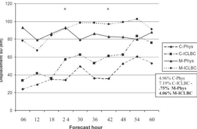
As with the other parameters, SDs of displacements from both techniques (Fig. 5) suggest a faster rate of growth for IC/LBC than for Phys, with the results for MODE being statistically significant. In addition, at most times, the SDs are larger in IC/LBC than in Phys. Per-haps most noticeable in Fig. 5 is the large difference in the magnitudes of the SDs between the two techniques. It is likely that these large differences in values are due to the fact that systems are only matched in CRA when they are contiguous, whereas in MODE, systems are matched if the interest parameter is greater than some
threshold. Thus, some systems are matched in MODE even though they are not contiguous and may be sepa-rated by some distance. Analysis of the first and last 6-h forecast periods from the 72 cases for a few of the en-semble members suggests that nearly half of the matched objects in MODE do not exhibit overlap. Average dis-placements for the two techniques (not shown) support this theory with CRA values generally between 100 and 150 km, and MODE values between 200 and 250 km at all times. The differences in the way the schemes operate should lead to larger average displacement errors and standard deviations in MODE than in CRA.
In summary, the trends toward increasing spread with time in the IC/LBC ensemble with less increase in the Phys ensemble seen in Clark et al. (2008) are observable in the four object parameters examined, and are espe-cially noticeable in both the MODE and CRA results for SDs of areal coverage. This result suggests that spread in areal coverage of forecasted precipitation systems is more sensitive to whether or not perturbed LBCs are used than spread in average rain rates, rain volumes, or displacement errors. For all four parameters, MODE finds spread to be greater in Phys at the early times and greater in IC/LBC at the later times; CRA only shows this for two parameters. Although the two techniques do not produce identical results, they do show the same general trends. CRA better shows differences between the two ensembles for the SDs of rain rate, while MODE shows more of a difference for SDs of rain volume. The diurnal cycle with precipitation being more abundant during the overnight hours has some influence on the SDs of these parameters, especially for rain rate, vol-ume, and areal coverage.
Because traditional spread measures such as variance are computed using point-to-point comparisons, they are influenced by precipitation amounts such that two ensemble forecasts with the same spatial distributions of rainfall among members but different predicted amounts FIG. 4. As in Fig. 2, but for areal coverage (number of
10 km310 km grid boxes) of rainfall.
will have different spreads. The fact that object-based techniques, which should not suffer the same influence, show the same temporal trends suggests that the Clark et al. (2008) findings are not an artifact of bias or other problems with traditional measures. Bias should affect some object parameters such as the average system area or rain volume directly and possibly also the average system rain rate. It may also influence the average dis-placement error, although such an influence would be less likely. Information from object-based techniques on these parameters can better define what the bias prob-lems are and assist with interpretation of traditional ensemble performance measures. However, if system-atic biases are present in an ensemble, the SDs of object parameters should be less affected by the biases than the traditional measure of variance. For instance, if one ensemble has a general high bias, it is likely most system rain volumes would be overestimated by most ensemble members, and there would be no particular reason why the SD for rain volume should be larger than that for a different ensemble with a smaller bias.
The diurnal signal seen in some of the object parameter SDs with relative maxima at the times of peak precipi-tation is similar to the trends noted for variance in Clark et al. (2008). However, in that study, maxima were present in both the MSEs and variances during the times of peak precipitation, with the MSEs showing a higher-amplitude signal. Although the object measures also showed maxima in the SDs at these times, the MSEs usually did not. This difference in results suggests that traditional computations of MSE, as performed in Clark et al. (2008), are influenced by bias or small displace-ments in forecasted heavy precipitation more than the object parameters examined in the present study.
4. Comparison of 4- and 20-km grid-spacing ensembles
To determine whether or not object parameters show the trends found in Clark et al. (2009) in a comparison of two ensembles using different grid spacing, MODE was used on 6-h accumulation periods covering 0000–0600, 0600–1200, 1200–1800, 1800–0000, and 0000–0600 UTC, or the 3–9-, 9–15-, 15–21-, 21–27-, and 27–33-h forecast periods, for the cases evaluated in that study. The com-parisons used five members for each ensemble, with the rainfall input into MODE on a 20-km grid. Because the results discussed in section 3 showed that both object-based verification techniques depicted the same general trends, the CRA method was not used on the ENS4 and ENS20 output.
The rain area (for amounts exceeding 6.25 mm) in terms of grid boxes (20 km320 km) averaged for all
objects identified in all ensemble members and SD of rain area, from both ENS4 and ENS20, and the observed rain area for each 6-h period are shown in Fig. 6. The diurnal minimum during the 1200–1800 UTC period can be seen in the observations, with higher values during the 0000–1200 UTC period. Both ensembles incorrectly show a peak during the 1800–0000 UTC period, and both show an overestimate (high bias) at all times. However, ENS4 has less of a high bias, is statistically significantly closer to the observations than ENS20 during the final forecast period, and does show a minimum during the 1200–1800 UTC period, unlike the 20-km ensemble. Both ensembles disagree most with the observations during the daylight hours (1200–0000 UTC).
SDs for the ensembles generally follow the same trends as the average rain area, with SDs for ENS20 larger than those for ENS4. During the last two periods, the rate of growth of spread is slightly larger in ENS4 than in ENS20. Additionally, the slope of the best-fit line applied to the data from all valid times is slightly greater for ENS4 than for ENS20, but the differences are not statistically sig-nificant. This faster growth of spread is consistent with Clark et al.’s (2009) finding of faster growth in ensemble variance in ENS4 compared to ENS20. Unlike the eq-uitable threat score (ETS) results discussed in Clark et al., the biggest improvements in the 4-km depiction of the rain area relative to ENS20 occurred during the 1200–1800 and 1800–0000 UTC periods, and not in the 0600–1200 UTC period when long-lived propagating convective systems are most common.
FIG. 6. Rain area (20 km320 km grid boxes) averaged for all objects in all ensemble members from MODE as a function of time for ENS4 (solid with squares) and ENS20 (solid with triangles), along with the observed value (dashed with asterisks) and the SDs for ENS4 (dotted with squares) and ENS20 (dotted with triangles). Slope of best-fit line for SD data, expressed as percentage change relative to average rain area SD, is shown in the inset. Asterisk at top indicates that errors compared to observations for ENS4 were statistically significantly less (p,0.05) than for ENS20.
Average rain rates for the ensembles and observa-tions, along with the SDs, are shown in Fig. 7. Both ensembles tended to predict the rain rate to within 10% of the observed value, much better agreement than was found for the rain area (Fig. 6). At all times except for the diurnal minimum (1200–1800 UTC), the two ensem-bles slightly overestimated the rates. The models cor-rectly depicted the times of the maxima and minima. The 4-km results were closer to the observed rates during the 0000–0600 UTC period, and then again in the last 12 h of the simulation, but no differences from ENS20 were statistically significant. At all times, ENS4 had more spread than ENS20, with a hint of faster growth of spread during the last 6–12 h of the forecast. However, the slopes of the best-fit lines for all of the data indicated less growth with time than for the SDs of the rain area, and slightly faster growth in spread for ENS20 than for ENS4, a result opposite to that for the rain area (Fig. 6) and what was found in Clark et al. (2009). Differences were not statistically significant, however. SDs were no more than 25% of the magnitude of the rain rates, a much smaller fraction than for the rain area (Fig. 6) where the SDs always exceeded 50% of the magnitudes of the average areas.
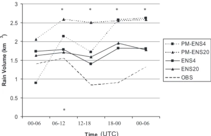
For rain volume (Fig. 8), as with rain area, both en-sembles showed a high bias at all times, with particularly large errors during the 1200–0000 UTC period. The di-urnal cycle is apparent in the observations, and ENS4 does a better job of showing the diurnal cycle, although both ensembles are too quick to increase the rain volume during the afternoon (1800–0000 UTC). Differences be-tween the average volumes were not statistically signifi-cant during any time period. The SDs follow the same trends as with rain area, with ENS20 having a greater SD at all times until the last 6 h, when ENS4 may be evi-dencing the faster error growth discussed in Clark et al. (2009). The slopes of the best-fit lines show the biggest difference in rate of growth with time for this parameter,
with ENS4 having a noticeably larger slope, but the differences were not statistically significant.
Clark et al. also noted that in Hovmo¨ller diagrams averaged over the model domain, the ENS20 mean computed using probability matching (PM; Ebert 2001) appeared to generate the diurnal maximum of day 2 too early and too intensely, and this result may be reflected in the peak in volume occurring in the ENS20 data be-tween 1800 and 0000 UTC (Fig. 8). PM is a statistical procedure whereby if we assume the best spatial repre-sentation of rainfall is given by the ensemble mean and the best frequency distribution of amounts is given by the model quantitative precipitation forecasts (QPFs), we can reassign the rain amounts from the ensemble mean using values randomly selected from the distri-bution of individual model QPFs. PM has been shown to correct for a large bias in rain area and underestimation of amounts caused by the averaging process used for the ensemble mean. The best agreement between both en-sembles and the observations does occur during the 0600–1200 UTC period, which is confirmed by the ETS values for the PM means in Clark et al. (2009). Because errors and SDs were relatively small for rain rate (Fig. 7), the larger values occurring for rain volume indicate that areal coverage of rainfall is a more troublesome fore-casting challenge for the ensemble members.
Average displacements and SDs of displacement for the two ensembles are shown in Fig. 9. ENS4 has less displacement error at all times, but differences com-pared to ENS20 were not statistically significant. Both ensembles have comparable SDs, roughly 50% of the magnitude of the displacements, and, unlike the other three parameters examined, growth in SDs with time is negligible. The displacement errors do not appear to reflect the diurnal cycle. Displacements in ENS4 were usually in the S or SW directions (not shown) through the 27-h forecast (0000 UTC) and then toward the NNE after that time (i.e., mean position of the forecasted objects FIG. 7. As in Fig. 6, but for rain rate (mm). FIG. 8. As in Fig. 6, but for rain volume (km3).
usually was SW of the observed one prior to hour 27). For ENS20, there were no systematic trends in the dis-placement direction.
In summary, the object parameters evaluated from MODE often supported the conclusions based on tradi-tional verification approaches applied to the 4- and 20-km ensembles. In particular, the object parameters indicated that ENS4 better depicted the diurnal cycle, and gener-ally had smaller errors at most times for most parameters than ENS20. There was also some evidence of the faster error growth found by Clark et al. (2009) with SDs grow-ing more rapidly in the ENS4 parameters than in the ENS20 ones. It must be noted, however, that unlike with the comparison of the Phys and IC/LBC ensembles, dif-ferences between the object parameters for ENS4 and ENS20 were rarely statistically significant. The analysis of object parameters also suggests that the average rain rate is forecasted better than the area, location, and volume, and that the variability in rain rate among members is less than it is for the other parameters.
5. Use of object-based verification parameters in ensemble forecasting
Because object-based verification techniques can pro-vide information on system parameters, it is possible that such techniques could be used to provide useful forecast information. As a preliminary exploration of how such information could be used to benefit forecasters, two tests were performed. First, CRA and MODE were applied to the ensemble mean precipitation forecast generated using PM applied to the various ensembles discussed earlier, and the skill levels of these forecasts of object parameters were compared to that of a forecast created by averaging the CRA and MODE output for parame-ters in each individual ensemble member. In a second
test, forecast skill was compared between a forecast for object parameters based on an average of the MODE output where objects in each ensemble member were defined using the 6.25-mm precipitation amount thresh-old (same technique used earlier in the present study), and a forecast where MODE objects were defined using a probability threshold applied to a probabilistic fore-cast created using equal weighting of the ensemble members. It should be kept in mind that in order to allow MODE and CRA to be used as a forecasting tool in real time, a user would not input observations to the tech-niques as is done for verification but could instead use a null field, substitute a particular forecast, or assume a perfect forecast in place of the observations. The pri-mary information needed from these codes would be the object parameters valid for systems depicted in the en-semble member forecasts.
a. Comparison of PM ensemble mean object parameters with averages of object parameters from all ensemble members
To investigate if a more skillful forecast could be achieved by applying object-based techniques to a PM ensemble mean forecast or by applying the techniques to each individual ensemble member and then averaging the object parameters, CRA was used on the two eight-member ensembles discussed in section 3, and MODE was used on the two five-member ensembles discussed in section 4.
Averages for each 6-h forecast period from CRA for the 72 cases for rain rate (not shown) indicated that objects in the PM forecast tended to have slightly lower rain rates at all hours than the average rain rate from objects identified in each of the eight ensemble members of the Phys ensemble, but the more accurate forecast was split evenly between these two approaches. For the IC/LBC ensemble the PM approach had the same or smaller errors than the average of the CRA results from all eight members about 70% of the time, but differences were usually small. For rain volume and displacement error (not shown), similar trends were noted with the PM forecast being comparable in skill to one based on an average of the parameter values from individual en-semble members. Thus, at least for these three param-eters, there would be little reason to average the output from object-based approaches run on every ensemble member. However, there may still be value in using the object-based approaches on each member to create distributions of possible scenarios (e.g., probabilities of rates, volumes, or displacements exceeding thresholds or falling within binned ranges).
A comparison of the areal coverage errors between forecasts using the PM mean and forecasts using averaging FIG. 9. As in Fig. 6, but for displacement (km), with no
of individual ensemble member areas (Fig. 10) reveals somewhat different behavior. At most times, the errors are more positive for the PM approach. A strong diurnal signal can be seen in the area errors with underestimates near the times of diurnal maxima in precipitation and overestimates at other times. Because the PM mean forecasts result in larger areas of precipitation, the agreement with the observations is generally worse ex-cept during the times of the diurnal maxima.
In another test of how the object-based output might be used to help forecasters, the percentage of the time that the observed rate, volume, and areal coverage fell within the spread of the two eight-member ensembles was examined during all 6-h forecast periods, which were grouped into day 1, 2, and 3 forecasts. Figure 11 shows that this approach worked much better for pre-dicting rain rate and volume than for areal coverage. For the rate and volume, the two ensembles captured the observed values roughly 50% of the time; for areal cov-erage the figure was closer to 10%. For all three param-eters, increasing skill with time was more pronounced in IC/LBC than in Phys, a result likely influenced by the faster growth in spread in IC/LBC (Clark et al. 2008).
An additional test was performed to see if a spread– skill relationship, where large spread was associated with less skillful forecasts, existed in the object parame-ters from the ensembles. Figure 12 shows the time evo-lution for the Phys ensemble of the mean absolute error for rain volume, rate, and areal coverage for those sys-tems that had large SDs among the members and those that had small values. Large and small were defined to be greater than 150% of the average SD or less than 50% of the average, respectively. Rain volume and areal coverage show a clear separation with much more
ac-curate forecasts in the events where spread is relatively small. Rain rate does not show the relationship as de-finitively, although for a majority of the time, it still applies. However, at hours 0–6, 18–24, and 48–60, the forecast skill either does not vary much with SD or the more accurate forecast is associated with larger SDs. It is not entirely clear why rain rate would behave differ-ently, although it should be pointed out that the SDs for rain rate are a much smaller fraction of the average magnitudes than those for the other parameters (not shown). Average rain rates at all times for both en-sembles are around 12 mm, so that the SDs (Fig. 2) are FIG. 10. Difference between the forecasted rain area and the
observed (10 km310 km grid boxes) as a function of time, based on CRA output for the mean value (solid lines with squares for Phys; triangles for IC/LBC), and the PM forecast (dotted lines with squares for Phys; triangles for IC/LBC).
FIG. 11. Percentage of time that observed values of rain volume (dashed line with squares for Phys; triangles for IC/LBC), rate (solid lines with squares for Phys; triangles for IC/LBC), and areal coverage (dotted lines with squares for Phys; triangles for IC/LBC) fell within the minimum and maximum predicted by the two en-sembles, based on CRA output. Day 1 refers to 6-h forecast periods in the first 18 h of the forecast, day 2 refers to those in the 18–42-h period, and day 3 those in the 42–60-h period.
FIG. 12. Mean absolute errors for volume (km3), rate (32.54 mm), and areal coverage (31000 grid boxes) of precipitation from CRA applied to Phys as a function of time for cases with SDs over 150% of the mean (squares with solid line for rate, dashed line for volume, and dotted line for area), and less than 50% of the mean (triangles with solid line for rate, dashed line for volume, and dotted line for area).
roughly 10% of the average values. Rain volumes are typically around 1 km3(not shown), so that SDs (Fig. 3) are often over 50% of these values. Likewise, SDs for areal coverage (Fig. 4) and displacement (Fig. 5) are often 50% or more of the typical values (not shown) of around 700 (MODE) to 800 (CRA) points and 100 km (CRA) to 200 km (MODE). These results in general imply that forecasters may be able to establish a confi-dence level for their forecasts of some object parameters using the SDs from ensembles. The same general ten-dencies were found for IC/LBC (not shown), with clearly better forecasts of rain volume and areal coverage when spread was small, but mixed results for rain rate.
As was done for the two eight-member 15-km en-sembles, a few tests were performed using MODE with ENS4 and ENS20 output to see if the average of a pa-rameter value from the set of ensemble members would be a better forecast than the parameter value from the PM ensemble mean. In Fig. 13, box and whisker plots show that the displacements using the PM approach have a wider distribution for both ENS4 and ENS20 than do the displacements determined by averaging MODE output from each ensemble member. For both ensembles, the median values of displacement for the PM approach are smaller than those for the average of
the ensemble members during the first three forecast periods, but differences become small at later times. The only statistically significant difference is for ENS4 dur-ing the 1200–1800 UTC period, however.
Different behavior is noted for the average rain areas (Fig. 14). For both ensembles, the forecasted rain areas are much closer to the observed values when the average of the areas from the individual ensemble members are used compared to the areas determined from the PM ensemble mean. The improvement is statistically signifi-cant at most times when 4-km grid spacing is used, and at one time when 20-km spacing is used. As was the case with Phys and IC/LBC, the areas in the PM mean forecast were larger than the average areas from the ensemble members. Because the ENS4 and ENS20 forecasts had a more persistent problem with overestimates of rainfall coverage, the PM forecasts of area were always worse than those obtained from averages of the individual ensemble members. The temporal trends in the average values of area still differ substantially from the observed diurnal cycle but do appear to be slightly more realistic than the trends associated with the PM forecast.
For rain rate (Fig. 15), the behavior was similar in both ensembles to rain area, with the average rate determined from the individual members being closer to the ob-served values than the PM ensemble mean, but the dif-ferences were not statistically significant. During the last 6 h of the forecast, there is some convergence of the curves so that the PM approach yields comparable re-sults to the averaging of individual members’ rain rates. FIG. 13. Box and whisker plots of MODE-determined
displace-ment error (km) for all cases as a function of forecast hour for ENS4 (average of all members shown with white boxes and PM ensemble mean shown with medium gray), and for ENS20 (average of all members shown with light gray boxes and PM ensemble mean with dark gray). Bottoms and tops of boxes show the 25th and 75th percentiles of the data, respectively, with the median indicated using a horizontal line, and whiskers covering the range of data to at most a distance of 1.5 interquartile ranges, with outliers shown using circles. Differences between the average value of the member-averaging technique and the PM approach statistically significant withp,0.05 are shown with asterisks at the top (for 4-km results) and bottom (for 20-km results) of the graph.
FIG. 14. Rain area (20 km320 km grid boxes) for the average of the 4-km ensemble members (solid line with squares) and the PM ensemble mean (dotted with squares), and for the average of the 20-km ensemble members (solid with triangles) and the 20-km PM ensemble mean (dotted with triangles), based on MODE output. Observations shown with dashed line. Differences in the errors (compared to observations) between the member-averaging tech-nique and the PM approach statistically significant withp,0.05 shown with asterisks at the top (for 4-km results) and bottom (for 20-km results) of the graph.
Note that the high bias for precipitation found by Clark et al. (2009) is apparent in both the rain area (Fig. 14) and rain rate (Fig. 15).
Because the rain volume should be equal to the rain rate multiplied by the rain area, the behavior of the curves in Fig. 16 is similar to that in Figs. 14 and 15. Once again, the average of rain volumes from individual en-semble members yields a value closer to that observed than what is obtained from the PM approach and the differences are statistically significant at most times for ENS4 and at one time for ENS20. It is interesting to note that a spinup delay observed in the 4-km ensemble output in Clark et al. (2009) does show up in the PM results (dotted curves) but not as much in the average of the rain volumes from all members. Differences between the two ensembles are amplified when using the average from all members during the first three forecast periods. These averages are much higher for ENS20 than ENS4. Overall, it appears that for displacement error using MODE with the 4- and 20-km ensemble output, the best forecast can be obtained by using the PM ensemble mean. However, for the parameters of areal coverage, rate, and volume of rainfall, better forecasts are possible by applying object-based verification tools to all ensemble members, and then averaging the parameter values from all members. Differences between the two approaches are less noticeable in the CRA results for the Phys and IC/LBC ensembles, although the averaging of individual member forecasts of areal coverage is more likely to yield a better forecast than that from the PM mean.
b. Comparison of results using MODE applied to ensemble probability forecasts and MODE applied to ensemble member forecasted precipitation amounts
Because MODE allows a user to compare objects gen-erated from two different fields, a test was performed
in which object parameters were obtained from both Phys and IC/LBC using probability of precipitation (POP) forecasts created using equal weighting of the eight mem-bers discussed in section 3 (thus, POP values could be 0%, 12.5%, 25%, 37.5%, etc). A probability threshold of 30% to define an object was tested, meaning that at least three of the eight members had to show precipitation above 6.25 mm in 6 h to be considered a system. A sen-sitivity test was also performed raising this threshold to 50%, which would mean that at least four members had to show an object.
Figure 17 compares the displacement errors using MODE applied to the POP forecasts to the errors when MODE was applied to the QPF amount with the results for all individual members averaged. In general, dis-placement errors grow with time. Also, the results using a 30% probability threshold are generally 5%–10% better than those based on the QPF amount. In the sensitivity test using a 50% threshold (not shown), dis-placement errors in the first 30 h average around 20 km worse for both ensembles, making them slightly worse than for the technique using the QPF amount. After hour 30, the results are mixed with the 50% threshold performing about the same as the 30% threshold, and actually being the best during the 54–60-h period. Future work should explore how the results change when dif-ferent probability thresholds are used, particularly for larger ensembles or more complex methods of determin-ing the probabilities.
Average rain areas for the two ensembles using both techniques with MODE are shown in Fig. 18, along with a curve representing the rain areas of the observed systems. It should be noted that since not all of the same observed areas get matched with forecasted systems, the observed area differs between the two ensembles. The observations curve plotted in Fig. 18 is an average of the MODE results for objects found using Phys and IC/ LBC. As mentioned earlier, none of the forecasts has as FIG. 15. As in Fig. 14, but for rain rate (mm).
strong a diurnal signal as the observations. Obviously, the threshold used for the probability forecast will greatly affect the rain areas depicted in the forecasted objects. Using 30% probabilities yields better results than those obtained when applying MODE to QPF amounts around the times of the diurnal maximum (0–6, 24–30, and 48–60 h), but this is likely primarily a result of the probability approach always yielding a much larger rain area (by 200–500 grid boxes at most times). The amplitude of the diurnal cycle is also a little stronger when the probability approach is used. When the prob-ability threshold was increased to 50%, areas decreased dramatically, as would be expected (not shown), and the curves looked more like those from the technique based on the QPF amount (solid lines). The diurnal signal was almost completely removed by changing the probability threshold in this manner. It should be noted that since more agreement is needed to have a 50% POP forecast, one might expect the numbers of systems identified to decrease as a higher POP threshold was used. However, a lower threshold could result in what had been several objects when a higher threshold was used combining into one larger object when the lower threshold was used. An examination of the numbers of objects found by MODE with the two thresholds did show that, at most times, substantially more objects were present when the 30% threshold was used (usually 10%–40% more), al-though for at least one time period, the two numbers were nearly identical.
Although not shown, one other interesting parameter computed using MODE on POP forecasts was the aver-age probability value for the forecasted objects. During the first 24 h, the Phys ensemble had probability values
roughly 5%–10% higher than those in IC/LBC. After 24 h, the differences increased with Phys typically being 15%–20% greater than IC/LBC. This result is consistent with IC/LBC having larger spread, such that POP fore-casts based on equal weighting of its members would have lower values. The same trends are apparent in the results based on a 50% probability threshold (not shown).
6. Conclusions
The use of object-based verification approaches to evaluate and enhance ensemble forecasts was tested by using both CRA and MODE on two sets of ensembles. The first set included an eight-member ensemble with mixed-physics and dynamic cores with unperturbed ICs and LBCs (Phys) and an eight-member ensemble with fixed-physics and perturbed ICs and LBCs (IC/LBC). Clark et al. (2008) found using traditional spread and skill measures that spread increased much faster in IC/LBC compared to Phys so that both spread and skill were better in IC/LBC than in Phys after roughly 24–30 h. The second set of ensembles included five members of a 4-km ensemble (ENS4) and five members of a 20-km ensemble (ENS20). Clark et al. (2009) found that a diurnal signal in precipitation was better depicted in ENS4, and this may have partly accounted for the better skill measures for ENS4 compared to ENS20. In addition, spread grew faster with time in ENS4.
Both CRA and MODE showed that in four object parameters studied—rain rate, volume, areal coverage, and displacement error—greater increases in spread with time occur in IC/LBC than in Phys, agreeing with Clark et al. (2008). Because the SDs of the object parameters should not be affected as much by systematic biases or small displacement errors in the position of heavy fore-casted rainfall as the traditional variance measure used by Clark et al., the present results add support to Clark FIG. 17. Comparison of displacement errors (km) by time
be-tween the two ensembles using the average of the MODE output applied to the QPF amount for all individual members (solid lines with squares for Phys; triangles for IC/LBC) and using MODE applied to probability forecasts with a 30% threshold (dotted lines with squares for Phys; triangles for IC/LBC).
FIG. 18. As in Fig. 17, but for rain area (10310 km grid boxes), and with the observed areas shown with the dashed line.
et al.’s conclusion. This trend for greater spread growth in IC/LBC was particularly noticeable in the areal cov-erage of precipitation systems, suggesting that spread in areal coverage of forecasted precipitation systems is more sensitive to whether or not perturbed lateral boundary conditions are used than spread in average rain rates, rain volumes, or displacement errors. Although the two object-based techniques do not produce identical re-sults, they do show the same general trends. The diurnal cycle with precipitation being more abundant during the overnight hours has some influence on the SDs of the object parameters examined, especially rain rate, vol-ume, and areal coverage. However, unlike in Clark et al. (2008), the diurnal cycle was less pronounced in MSE for object parameters, implying less impact from biases or displacements in forecasted rain regions from those observed.
In a comparison of object parameters derived from MODE for ENS4 and ENS20, ENS4 was found to better depict the diurnal cycle and, generally, had smaller er-rors at most times for most parameters than ENS20. There was also some evidence of the faster error growth found by Clark et al. (2009), with standard deviations growing more rapidly in the ENS4 parameters than in the ENS20 ones. Unlike with Phys and IC/LBC, how-ever, the differences between ENS4 and ENS20 were usually not statistically significant, possibly a result of both a smaller sample size and a shorter period of in-tegration. The standard deviations were much smaller for rain rate than for other parameters, and agreement with the observations was also best for rain rate.
Several tests were also performed to examine methods of using object-based verification output to assist fore-casters. It was found that predictions of the areal cov-erage of precipitation systems are more accurate when based on the average of the predicted areas from each ensemble member as opposed to using a PM ensemble mean forecast input into the object-based techniques. For the other parameters (i.e., rain rate, volume, and displacement), differences in the skill of both approaches were less substantial. It was also found that object-based approaches making use of probability thresholds to de-fine precipitation systems could yield forecasts of object parameters equally skillful to those based on a precipi-tation amount threshold.
The present study is a preliminary look at how object-based approaches could be applied to ensemble fore-casts, and much additional work is needed. Most of the cases examined here consisted of convective systems in the central United States. Analysis should be performed on larger-scale cold season events covering other areas. In addition, the present study emphasized deterministic information obtained from ensembles, such as the
av-erage rain volume or areal covav-erage. Future work should examine probabilistic forecasts of object parameters, and expand the number of parameters analyzed. Sensitivity to user-defined parameters within the object-based verifi-cation techniques should also be explored further.
Acknowledgments.This research was funded in part by National Science Foundation Grants ATM-0537043 and ATM-0848200, and also by the WRF DTC. Special thanks are given to John Halley Gotway and Randy Bullock for assistance with MODE and methods of an-alyzing MODE output. Adam Clark kindly provided the precipitation output analyzed, and also provided useful feedback on the manuscript. Additional help was pro-vided by Jon Hobbs, Daryl Herzmann, James Correia, Elizabeth Ebert, Barbara Brown, Louisa Nance, and Pam Johnson. The author would like to thank Bob Gall and the entire WRF-DTC leadership group for the op-portunity to visit at the DTC and share in stimulating discussions there. The paper was improved through the constructive comments of three anonymous reviewers.
REFERENCES
Baldwin, M. E., and J. S. Kain, 2006: Sensitivity of several perfor-mance measures to displacement error, bias, and event fre-quency.Wea. Forecasting,21,636–648.
Betts, A. K., 1986: A new convective adjustment scheme. Part I: Observational and theoretical basis. Quart. J. Roy. Meteor. Soc.,112,677–691.
——, and M. J. Miller, 1986: A new convective adjustment scheme. Part II: Single column tests using GATE wave, BOMEX, ATEX and Arctic air-mass data sets.Quart. J. Roy. Meteor. Soc.,112,693–709.
Casati, B., and Coauthors, 2008: Forecast verification: Current status and future directions.Meteor. Appl.,15,3–18.
Chapman, M., R. Bullock, B. G. Brown, C. A. Davis, K. W. Manning, R. Morss, and A. Takacs, 2004: An object-oriented approach to quantitative precipitation forecasts: Part II—Examples. Pre-prints,17th Conf. on Probability and Statistics in the Atmospheric Sciences/20th Conf. on Weather Analysis and Forecasting/16th Conf. on Numerical Weather Prediction,Seattle, WA, Amer. Meteor. Soc., J12.5. [Available online at http://ams.confex. com/ams/pdfpapers/70881.pdf.]
Clark, A. J., W. A. Gallus Jr., and T.-C. Chen, 2008: Contributions of mixed physics versus perturbed initial/lateral boundary conditions to ensemble-based precipitation forecast skill.Mon. Wea. Rev.,136,2140–2156.
——, ——, and M. Xue, 2009: A comparison of precipitation forecast skill between small convection-resolving and large non-convection-resolving ensembles. Wea. Forecasting, 24,
1121–1140.
Davis, C., B. Brown, and R. Bullock, 2006a: Object-based verifi-cation of precipitation forecasts. Part I: Methodology and application to mesoscale rain areas. Mon. Wea. Rev., 134,
1772–1784.
——, ——, and ——, 2006b: Object-based verification of pre-cipitation forecasts. Part II: Application to convective rain systems.Mon. Wea. Rev.,134,1785–1795.
Dyer, A. J., and B. B. Hicks, 1970: Flux-gradient relationships in the constant flux layer.Quart. J. Roy. Meteor. Soc., 96,
715–721.
Ebert, E. E., 2001: Ability of a poor man’s ensemble to predict the probability and distribution of precipitation.Mon. Wea. Rev.,
129,2461–2480.
——, and J. L. McBride, 2000: Verification of precipitation in weather systems: Determination of systematic errors.J. Hy-drol.,239,179–202.
——, and W. A. Gallus Jr., 2009: Toward better understanding of the contiguous rain area (CRA) method for spatial forecast verification.Wea. Forecasting,24,1401–1415.
——, L. J. Wilson, B. G. Brown, P. Nurmi, H. E. Brooks, J. Bally, and M. Jaeneke, 2004: Verification of nowcasts from the WWRP Sydney 2000 Forecast Demonstration Project.Wea. Forecasting,19,73–96.
Ferrier, B. S., Y. Jin, Y. Lin, T. Black, E. Rogers, and G. DiMego, 2002: Implementation of a new grid-scale cloud and rainfall scheme in the NCEP Eta model. Preprints, 15th Conf. on Numerical Weather Prediction, San Antonio, TX, Amer. Meteor. Soc., 280–283.
Gilleland, E., D. Ahijevych, B. G. Brown, B. Casati, and E. E. Ebert, 2009: Intercomparison of spatial forecast verification methods. Wea. Forecasting,24,1416–1430.
Grams, J. S., W. A. Gallus Jr., L. S. Wharton, S. Koch, A. Loughe, and E. E. Ebert, 2006: The use of a modified Ebert–McBride technique to evaluate mesoscale model QPF as a function of convective system morphology during IHOP 2002. Wea. Forecasting,21,288–306.
Grell, G. A., and D. Devenyi, 2002: A generalized approach to pa-rameterizing convection combining ensemble and data assimi-lation techniques. Geophys. Res. Lett.,29,1693, doi:10.1029/ 2002GL015311.
Hong, S.-Y., and J.-O. J. Lim, 2006: The WRF single-moment 6-class microphysics scheme (WSM6).J. Kor. Meteor. Soc.,42,
129–151.
Janjic´, Z. I., 1994: The step-mountain Eta coordinate model: Fur-ther developments of the convection, viscous sublayer, and turbulence closure schemes.Mon. Wea. Rev.,122,927–945. ——, 1996: The surface layer in the NCEP Eta model. Preprints,
11th Conf. on Numerical Weather Prediction,Norfolk, VA, Amer. Meteor. Soc., 354–355.
——, 2002: Nonsingular implementation of the Mellor–Yamada level 2.5 scheme in the NCEP Meso Model. NCEP Office Note 437, 61 pp.
——, 2003: A nonhydrostatic model based on a new approach. Meteor. Atmos. Phys.,82,271–285.
Kain, J. S., and J. M. Fritsch, 1993: Convective parameterization for mesoscale models: The Kain–Fritsch scheme.The Represen-tation of Cumulus Convection in Numerical Models, Meteor. Monogr.,Amer. Meteor. Soc., No. 46, 165–170.
Mass, C. F., D. Ovens, K. Westrick, and B. A. Colle, 2002: Does increasing horizontal resolution produce more skillful fore-casts?Bull. Amer. Meteor. Soc.,83,407–430.
Mellor, G. L., and T. Yamada, 1982: Development of a turbulence closure model for geophysical fluid problems.Rev. Geophys.,
20,851–875.
Monin, A. S., and A. M. Obukhov, 1954: Basic laws of turbulent mixing in the surface layer of the atmosphere (in Russian). Contrib. Geophys. Inst. Acad. Sci. USSR,151,163–198. Noh, Y., W. G. Cheon, S.-Y. Hong, and S. Raasch, 2003:
Im-plementation of the K-profile model for the planetary boundary layer based on large eddy simulation data. Bound.-Layer Meteor.,107,401–427.
Paulson, C. A., 1970: The mathematical representation of wind speed and temperature profiles in the unstable atmospheric surface layer.J. Appl. Meteor.,9,857–861.
Skamarock, W. C., J. B. Klemp, and J. Dudhia, 2001: Prototypes for the WRF (Weather Research and Forecasting) model. Pre-prints,Ninth Conf. on Mesoscale Processes,Fort Lauderdale, FL, Amer. Meteor. Soc, J15. [Available online at http://ams. confex.com/ams/pdfpapers/23297.pdf.]
Tartaglione, N., S. Mariani, C. Accadia, A. Speranza, and M. Casaioli, 2005: Comparison of rain gauge observations with modeled precipitation over Cyprus using contiguous rain area analysis.Atmos. Chem. Phys.,5,2147–2154.
Thompson, G., R. M. Rasmussen, and K. Manning, 2004: Explicit forecasts of winter precipitation using an improved bulk mi-crophysics scheme. Part I: Description and sensitivity analysis. Mon. Wea. Rev.,132,519–542.
Webb, E. K., 1970: Profile relationships: The log-linear range and extension to strong stability.Quart. J. Roy. Meteor. Soc.,96,
67–90.
Xue, M., and Coauthors, 2007: CAPS realtime storm-scale en-semble and high-resolution forecasts as part of the NOAA Hazardous Weather Testbed 2007 spring experiment. Pre-prints,22nd Conf. on Weather Analysis and Forecasting/18th Conf. on Numerical Weather Prediction,Park City, UT, Amer. Meteor. Soc., 3B.1. [Available online at http://ams.confex. com/ams/pdfpapers/124587.pdf.]