Approximate Joint Diagonalization within the
Riemannian Geometry Framework
Florent Bouchard, Louis Korczowski, J´
erˆ
ome Malick, Marco Congedo
To cite this version:
Florent Bouchard, Louis Korczowski, J´
erˆ
ome Malick, Marco Congedo. Approximate Joint
Di-agonalization within the Riemannian Geometry Framework. 24th European Signal Processing
Conference (EUSIPCO 2016), Aug 2016, Budapest, Hungary.
<
hal-01370052
>
HAL Id: hal-01370052
https://hal.archives-ouvertes.fr/hal-01370052
Submitted on 21 Sep 2016
HAL
is a multi-disciplinary open access
archive for the deposit and dissemination of
sci-entific research documents, whether they are
pub-lished or not.
The documents may come from
teaching and research institutions in France or
abroad, or from public or private research centers.
L’archive ouverte pluridisciplinaire
HAL
, est
destin´
ee au d´
epˆ
ot et `
a la diffusion de documents
scientifiques de niveau recherche, publi´
es ou non,
´
emanant des ´
etablissements d’enseignement et de
recherche fran¸
cais ou ´
etrangers, des laboratoires
publics ou priv´
es.
Approximate Joint Diagonalization within the
Riemannian Geometry Framework
Florent Bouchard
∗, Louis Korczowski
∗, J´erˆome Malick
†, Marco Congedo
∗∗GIPSA-lab, CNRS, Univ. Grenoble Alpes, Grenoble Institute of Technology, Grenoble France †LJK, CNRS, Univ. Grenoble Alpes, Grenoble France
Email: [email protected]
Abstract—We consider the approximate joint diagonalization problem(AJD) related to the well knownblind source separation
(BSS) problem within the Riemannian geometry framework. We define a new manifold named special polar manifold equivalent to the set of full rank matrices with a unit determinant of their Gram matrix. The Riemannian trust-region optimization algorithm allows us to define a new method to solve the AJD problem. This method is compared to previously published NoJOB and UWEDGE algorithms by means of simulations and shows comparable performances. This Riemannian optimization approach thus shows promising results. Since it is also very flexible, it can be easily extended to block AJD or joint BSS.
Index Terms—approximate joint diagonalization; blind source separation; Riemannian geometry; Riemannian optimization; special polar manifold
I. INTRODUCTION
Theapproximate joint diagonalization(AJD) of a matrix set is instrumental to solve the well knownblind source separation
(BSS) problem [1]. It can be expressed as it follows: given a set ofKsymmetric matrices{Ck}1≤k≤K of dimensionn×n,
find a full-rank matrixBof dimensionn×p(withp≤n) such that the set{BTC
kB}1≤k≤K contains matrices as diagonal as
possible according to some criterion.
A common diagonality criterion is the sum of squares of the off-diagonal elements of the transformed matrices leading to the minimization of the functional
f(B) = K X k=1 off(BTCkB) 2 F , (1)
whereB∈Rnp,k.kF denotes the Frobenius norm andoff(·)
vanishes the diagonal elements of its argument.
While optimizing (1), we need to avoid the trivial solution
B = 0. Hence, some constraints on the joint diagonalizer are usually added. A common choice is to fix the norm of the columns of B [2]–[4]. Another solution, when B is square (p =n), is to fix its determinant as proposed in [5]. In this paper, we generalize this latter constraint to the non-square case by fixing the determinant of the Gram matrix BTB of
B.
Even though the AJD has already been extensively studied, proposed method are usually very specific to a cost function, a constraint and an optimization algorithm. Here, we propose a general framework based on Riemannian geometry that can handle various cost functions and optimization algorithms.
Furthermore, except those methods that seek an orthogonal diagonalizer [6] or that do not ensure full rank property [4], existing algorithms can only deal with square joint diagonal-izer. If one wants to apply adimension reductionin this case, a
whiteningstep is mandatory [1], [7]. Such approach has been shown suboptimal [6]. Hence, to the best of our knowledge, we propose here the first method without severe limitations that can properly handle dimension reduction.
The aim of this paper is to show that it is possible to tackle the AJD problem within theRiemannian geometry framework. This allows to turn constrained optimization problems on embedded spaces into unconstrained problems on smooth manifolds[8]. The idea is to use thegeometrical propertiesof the constraints to define asmooth manifoldwhere the problem is not constrained anymore. This allows to handle constraints in a natural way. Riemannian approaches for AJD have already been considered for example in [4]–[6]. Moreover, a link between the Riemannian geometric mean of a set and its AJD has been recently found [9]. None of proposed Riemannian AJD methods suit well our purpose. They either make use of unadapted manifolds as in [4], [6] (see above) or only elements of Riemannian geometry are used and not the all framework as in [5]. In this article, we define an appropriate manifold for the AJD problem. In the following, we consider
p≤n. The manifold defined here is equivalent to the space
Bp,n={B ∈Rnp∗ : det(BTB) = 1} whereRnp∗ is the set of full rank matrices anddet(.)denotes the determinant.
This paper is divided into four sections including this intro-duction. In Section II-A, tools needed to perform optimization within the Riemannian framework are briefly introduced (see [8] for details). In Section II-B, The well-knownStiefel man-ifold [8] is presented. In Section II-C, a new manifold called
special symmetric positive definite manifoldis defined and its geometry is studied. The product of those two manifolds leads to a new manifold named special polar manifold in Section II-D. This latter manifold is shown to be equivalent to Bp,n
defined above using thepolar decomposition. In Section II-E, the objective function (1) is defined for the special polar manifold and its gradient and Hessian are derived. Then, the Riemannian trust-region method, which is chosen here as the optimization scheme, is presented in Section II-F. In Section III, the performance of the proposed method is analyzed and compared to state-of-the-art AJD algorithms [2], [3]. Finally, in Section IV, conclusions are drawn.
II. METHOD
A. Tools for Optimization on Riemannian Manifolds
Riemannian optimization methods search for the next iterate in the tangent space of the current iterate using Riemannian differential geometry tools (Riemannian gradient,Riemannian Hessian). The solution in thetangent space is then projected back onto the manifold. In order to solve optimization prob-lems within the Riemannian framework [8] one needs to define the following mathematical objects:
• theprojection mapthat projects a point of the embedded space onto the tangent space at a given point of the manifold;
• a suitable Riemannian metricon the tangent space; • the Levi Civita connection, which is essential to be able
to define the Riemannian Hessianof a function; • aretraction, which is a mapping from the tangent space
back onto the manifold.
B. Stiefel Manifold
The Stiefel manifold Stp,n ={U ∈ Rnp : UTU =Ip} is
well known. The reader is referred to [8] for proofs of the following:
Stp,n is an embedded submanifold of the Euclidean space
Rnp of dimension np−12p(p+ 1). Its tangent space at U is
TUStp,n ={ξ ∈Rnp :UTξ+ξTU = 0} endowed with the
metric gU such that, for allξandη inTUStp,n,
gU(ξ, η) = tr(ξTη), (2)
where tr(M) denotes the trace of M. For any matrix Z in
Rnp, the projection mapPU onTUStp,n is given by
PU(Z) =Z−Usym(UTZ), (3)
wheresym(M) = 12(M +MT). The Levi Civita connection
∇ atU in Stp,n is defined, for η inTUStp,n andξ in the set
of vector fields on Stp,n denotedX(Stp,n), as
∇ηξ= PU(Dξ(U)[η]) (4)
where Dξ(U)[η] denotes the directional derivative of ξ atU
in the direction η. A retractionRU is properly defined, for all
ξ inTUStp,n, by
RU(ξ) = qf(U+ξ), (5)
where qf(M) returns the Qfactor of the QR decomposition of M.
C. Special Symmetric Positive Definite Manifold
Let Sp (respectively Sp++) denotes the manifold of
sym-metric (respectively symsym-metric positive definite) matrices. We define here the Special Symmetric Positive Definite manifold
Wp as the set{S∈ Sp++ : det(S) = 1}.
Proposition 1. Wp is an embedded submanifold of Sp++ of dimension 12p(p+ 1)−1.
Proof. Wp is a subset of Sp++ by definition. Consider the
function F defined for all S in S++
p as F(S) = det(S).
Clearly, the image of F is R+∗ and Wp = F−1({1}). Let S
inWp andX inRpp, the directional derivative of F atS in
the direction of X is DF(S)[X] = tr(S−1X). Let x in
R+∗, then X = xpS is in S++
p and DF(S)[X] = x. This shows
thatFis a submersion. Proposition 3.3.3 in [8] completes the
proof.
Proposition 2. Wp is a connected manifold. Proof. Consider the geodesic of S++
p defined for allS1 and
S2such that for alltin[0,1],γ(t) =S
1/2 1 (S −1/2 1 S2S −1/2 1 ) tS1/2 1 [10], where(·)tis the power t. If S1 andS2 are in Wp then
for allt,det(γ(t)) = 1. This is a consequence ofdet(M N) = det(M) det(N)anddet(Mt) = (det(M))t. It follows that for
allS1 andS2 inWp there exists a path inWp that connects
them.
Proposition 3. The tangent space of Wp at S is TSWp =
{X ∈ Sp: tr(S−1X) = 0}endowed with the metricegS such that, for allξand η inTSWp,egS(ξ, η) = tr(S
−1ξS−1η).
Proof. First note that sinceWp is an embedded submanifold
of S++
p , it follows from Section 3.6.1 of [8] that TSWp is a
subset ofTSSp++=Sp [10]. Then, consider functionF(S) =
det(S) again. The kernel of DF(S) is the set {X ∈ Sp :
tr(S−1X) = 0}. Equation (3.19) in [8] allows to conclude that this corresponds toTSWp. Finally, the Riemannian metric
e
gS is inherited fromS++
p [10].
Proposition 4. For all Z in Rpp, the projection map PeS on
TSWp is given byPeS(Z) = sym(Z)−1ptr(S−1sym(Z))S Proof. It is straightforward to check that PeS verifies the
properties of the projection map.
Proposition 5. The Levi Civita connection ∇e at S in Wp is defined, for η in TSWp and ξ in X(Wp), as ∇eηξ =
e
PS(Dξ(S)[η]−sym(ηS−1ξ)).
Proof. Since Wp is a submanifold of Sp++, it follows from
Proposition 5.3.2 in [8] that∇eηξ=PeS(∇bηξ)where∇b is the
Levi Civita connection ofS++
p . Using the expression of∇b that
can be found in Appendix B of [11] completes the proof.
Proposition 6. A retraction ReS is properly defined, for allξ inTSWp, byReS(ξ) =S1/2exp(S−1/2ξS−1/2)S1/2.
Proof. ReS defines a retraction on Sp++. Furthermore, if
det(S) = 1, then det(ReS(ξ)) = 1 for any ξ inTSWp. This
comes from the fact that det(exp(M)) = exp(tr(M)) and
tr(M N) = tr(N M). This is enough to conclude.
D. Special Polar Manifold
We are finally ready to define the manifold of interest. Let us name Mp,n = Stp,n× Wp the Special Polar manifold.
First, we will investigate the link between Mp,n andBp,n.
Proposition 7. The mapping π : (U, S) 7→ U S is a one to one correspondance between the elements ofMp,n and those ofBp,n (usually denotedMp,n' Bp,n).
Proof. The polar decomposition ofBinBp,ncan be uniquely
defined such that B =U S where U is in Stp,n andS is in
S++
p . One can show that since det(S)>0, det(BTB) = 1
if and only if det(S) = 1. This shows that the mapping π
defined from Mp,n toBp,n is bijective.
As it is a product of Riemannian manifolds, Mp,n is a
Riemannian manifold [8]. Due to this fact, the proofs of the following are immediate. The tangent space ofMp,n atB=
(U, S) is TBMp,n = TUStp,n ×TSWp endowed with the
metric gB such that, for allξ= (ξU, ξS)andη= (ηU, ηS)in
TBMp,n,
gB(ξ, η) = gU(ξU, ηU) +egS(ξS, ηS). (6)
For all Z = (ZU, ZS) inRnp×Rpp, the projection map PB
atB = (U, S)onTBMp,n is given by
PB(Z) = (PU(ZU),PeS(ZS)). (7)
The Levi Civita connection ∇ at(U, S) inMp,n is defined,
for η= (ηU, ηS)andξ= (ξU, ξS), as
∇ηξ= (∇ηUξU,∇eηSξS). (8)
A retractionRBatB= (U, S)is defined, for allξ= (ξU, ξS),
by
RB(ξ) = (RU(ξU),ReS(ξS)). (9) E. The Objective Function onMp,n
In order to perform AJD on Mp,n within the Riemannian
framework, we need to define the objective function along with its Riemannian gradient and Hessian on the manifold.
1) Objective Funtion: Using the mapping πdefined in the previous section, one can easily find that the cost function f
on Mp,n corresponding to (1) is defined as f(U, S) = K P k=1 off((U S)TCkU S) 2 F = K P k=1 tr(off((U S)TCkU S)(U S)TCkU S). (10) Letˆfdenotes the same function defined onRnp×Rpp rather
than on Mp,n. f is then the restriction of ˆf to Mp,n. This
latter functionˆfwill be useful to obtain the gradient and the Hessian of f.
2) Gradient: The gradient offatB = (U, S)inMp,n,
de-notedgrad f(B), corresponds to the only element ofTBMp,n
such that for allξ inTBMp,n,gB(grad f(B), ξ) = Df(B)[ξ]
[8].
In practice, it is simpler to find grad ˆf(B), the gradient of
ˆf at B = (U, S) inRnp×Rpp and then deduce grad f(B).
Basic calculations lead to
D ˆf(B)[ξ] = K P k=1 4 tr(ξT UCkU Soff((U S)TCkU S)ST) + K P k=1 4 tr(ξT SUTCkU Soff((U S)TCkU S)). (11) It follows that grad ˆf(B) = K P k=1 4CkU Soff((U S)TCkU S)ST, K P k=1 4UTC kU Soff((U S)TCkU S) . (12)
Finally, by denoting grad ˆf(U) (respectively grad ˆf(S)) the first (respectively the second) component of grad ˆf(B), one can check that grad f(B)is properly defined as
grad f(B) = PU(grad ˆf(U)),
e
PS(Ssym(grad ˆf(S))S)
. (13)
3) Hessian: The Riemannian Hessian [8] offatBinMp,n
is the linear mapping defined for allξ= (ξU, ξS)inTBMp,n
byHess f(B)[ξ] =∇ξgrad f, which is still inTBMp,n.
Here again it is possible to findHess ˆf(B)and then deduce
Hess f(B). One can show thatHess ˆf(B)is given by
Hess ˆf(B)[Z] = D grad ˆf(B)[Z] = K P k=1 4Ck( ˙V MkST +VM˙kST +V MkZST), K P k=1 4ZT UCkV Mk+ 4UTCk( ˙V Mk+VM˙k) , (14) where Z = (ZU, ZS) is in Rnp×Rpp, V = U S, V˙ =
ZUS+U ZS, Mk = off(VTCkV)andM˙k = off( ˙VTCkV +
VTCkV˙).
The first (respectively second) component ofHess f(B)[ξ]
is denotedHess f(U)[ξ](respectivelyHess f(S)[ξ]) whereξis inTBMp,n. The same notations are used forˆf. It follows that
Hess f(U)[ξ] = PU(Hess ˆf(U)[ξ]) − PU(ξUsym(UTgrad ˆf(U))) Hess f(S)[ξ] = PeS(Ssym(Hess ˆf(S)[ξ])S) + 2PeS(ξSsym(grad ˆf(S))S) + PeS(DPeS[ξS](Ssym(grad ˆf(S))S)) − PeS(sym(ξSS−1grad f(S))), (15) where for all ZsinRpp andξS inTSWp
DePS[ξS](ZS) = 1ptr(S−1ξSS−1sym(ZS))S − 1 ptr(S −1sym(Z S))ξS . (16)
F. The Trust-Region Method
We will minimizef over the manifoldMp,n by a standard
second-order Riemannian optimization algorithm, the Riem-mannian trust-region method [8]. We sketch here the main idea of this algorithm and refer to Chapter 7 in [8] for more details. Starting from an initial pointB0 inMp,n, a sequence
of iterates{Bl}is computed in order to find a minimizer to the
cost functionf. To do so, a modelmBl offaround the iterate
Blis constructed using the second-order Taylor expansion for
ξinTBlMp,n such as
mBl(ξ) = f(Bl) + gBl(grad f(Bl), ξ)
+12gBl(Hess f(Bl)[ξ], ξ).
This model is considered to be valid in a trust-region defined as a ball inTBlMp,n with radius∆l. It is then needed to find
the solution ξl to the subproblem of minimizing mBl within
the ball of radius∆lin the tangent space ofBl. This is done
using the truncated conjugate-gradient method. The candidate next iterate is then RBl(ξl). This candidate is evaluated to
check that the model mBl atξl is valid. If it is the case, the
candidate is accepted and the radius∆lcan even be increased
if the model is very good. Otherwise, the candidate is rejected and∆l is decreased. The stopping criterion is defined by the
norm of the Riemannian gradient lower than a tolerance (fixed at10−5 in our numerical experiments).
III. RESULTS
In order to estimate the perfomances of our method, named RAJD (for Riemannian AJD), we simulated data and compared it to NoJOB [2] and UWEDGE [3]. RAJD was performed using manopt toolbox [12] in Matlab (c) with modifications in order to use the new manifold defined here.
To analyze how the methods behaved, we used two criteria. The first one is the Moreau-Amari indexIM-A [13] defined as
IM-A= 2n(n1−1) n P i=1 n P j=1 |Hij| max 1≤j≤n|Hij| −1 + n P j=1 n P i=1 |Hij| max 1≤i≤n| Hij|−1
whereH=BTA, withB the estimated unmixing matrix and
A the true mixing matrix. The second one is a measure of non-diagonalityIn-d of the transformed dataset defined as
In-d= 1 K(n−1) K X k=1 off(BTCkB) 2 F kdiag(BTC kB)k 2 F
wherediag(M)denotes the diagonal part of the matrixM. We performed 200 tests. For each test, as it is done in [3], we generated K = 100 matrices {Ck}1≤k≤K of dimension
n×naccording to Ck =ADkAT+ 1 2σ(Nk+N T k)
where A is a non-orthogonal mixing matrix with i.i.d. el-ements generated from a normal distribution N(0,1). We controlled the non-orthogonality by constraining the condition number with respect to inversion between 3 and 7. Matrices
{Dk}1≤k≤K are diagonal with i.i.d. elements generated from
a chi-squared distribution corresponding to the power of the sources in the BSS problem. σ is a free parameter defining the noise level and Nk is a noise matrix with elements
drawn independently from a normal distribution N(0,1). No dimension reduction was performed (i.e., p = n) and all algorithms were initialized with the identity.
In figure 1, the Moreau-Amari index IM-A of the three
methods for n = 8 as a function of the noise parameter σ
is presented. One can see that all three methods have similar behaviours even though UWEDGE gives, in general, results
Fig. 1. Median and quantiles (5% and 95%) over 200 tests of the Moreau-Amari index as a function of the noise parameter σfor the three methods forn= 8. All three methods have comparable performance. UWEDGE have slightly better results. See text for details.
Fig. 2. Median and quantiles (5% and 95%) over 200 tests of the non-diagonality measure as a function of the noise parameter σ for the three methods forn= 8. Again, all three methods have comparable results. RAJD diagonalizes the datasets better than the other methods. See text for details.
slightly closer to the true solution. In figure 2, we plotted the non diagonality measure In-d as a function of the noise
parameter σ for all methods for n = 8. It can be noticed that here RAJD diagonalized the datasets better. Even though RAJD and NoJOB succeeded better in diagonalizing the datasets, the solutions found by UWEDGE are generally closer to the true solutions. This reflects the fact that when noise is added, the true solution does not necessarily correspond to the one that diagonalizes the dataset better.
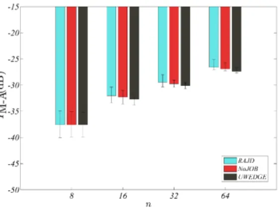
In figures 3 and 4, we studied the effect of the dimension
n of the matrices Ck for the three methods for σ = 100.
As expected, the results deteriorate when nincreases for all methods. Moreover, we still have comparable performance for all methods and it is consistent with results obtained when the influence of the noise was studied. Indeed, the joint diagonalizer of UWEDGE is generally slightly closer to the true solution (see figure 3) and RAJD diagonalizes the datasets better (figure 4). This shows that RAJD is still a valid method when the dimension of the problem is increased.
RAJD and NOJoB use the same cost function (1) but the cost function of UWEDGE is slightly different [3]. Our results
Fig. 3. Median and quantiles (5% and 95%) over 200 tests of the Moreau-Amari index as a function of matrices dimension nfor the three methods forσ= 100. The performance decreases when the dimension increases. All methods have comparable performances. See text for details.
Fig. 4. Median and quantiles (5% and 95%) over 200 tests of the non-diagonality measure as a function of matrices dimension n for the three methods for σ = 100. The performance decreases when the dimension increases. All methods have comparable performances. See text for details.
suggest that objective function (1) leads to an overfitting of the data. This indicates that the Riemannian method that we considered is efficient in minimizing (1) but this function seems not to be well suited for our purpose. Furthermore, the fact that RAJD gave better results for In-d than NOJoB,
which uses the same cost function, suggest that Riemannian optimization on the special polar manifold is a promising tool. The use of a more appropriate cost function may lead to better results as compared to state of the art methods such as UWEDGE.
IV. CONCLUSION
In this article we have properly defined the special polar manifold allowing the investigation of the AJD problem from a Riemannian optimization point of view. Of course, this new manifold may turn useful in many other problems. The results we obtained for the AJD problem are encouraging and the limits encountered seems to be related to objective function we have considered. Other cost functions such as the ones in [3] or [14] are under consideration and will be presented
in future works. Other Riemannian optimization algorithms can also be investigated. Note that since accuracy is sought here, second order algorithms (usingRiemannian Hessian or approximation of it) should be preferred. We are also interested in studying direct dimension reduction allowing to avoid the usualwhiteningstep, with possible gain in precision.
This study shows that working within the Riemannian geometry framework is appropriate to solve the AJD problem. Furthermore, unlike the strategies discussed in the introduc-tion, this approach allows to easily change the optimization scheme or the cost function, as long as this latter is smooth. Other related models can also simply be considered such as extensions to block AJD or joint BSS [7].
ACKNOWLEDGMENT
The authors would like to thank Bijan Afsari for his helpful comments on this work. This work has been partially sup-ported by the LabEx PERSYVAL-Lab (ANR-11-LABX-0025-01) funded by the French program “Investissement d’avenir” and the European Research Council project CHESS 2012-ERC-AdG-320684.
REFERENCES
[1] P. Comon and C. Jutten. Handbook of Blind Source Separation: Independent Component Analysis and Applications. Academic Press, 1st edition, 2010.
[2] M. Congedo, R. Phlypo, and J. Chatel-Goldman. Orthogonal and non-orthogonal joint blind source separation in the least-squares sense. In 20th European Signal Processing Conference (EUSIPCO-2012), pages 1885–1889, 2012.
[3] P. Tichavsk`y and A. Yeredor. Fast approximate joint diagonalization incorporating weight matrices. Signal Processing, IEEE Transactions on, 57(3):878–891, 2009.
[4] P.-A. Absil and K.A. Gallivan. Joint diagonalization on the oblique manifold for independent component analysis. In Acoustics, Speech and Signal Processing, 2006. ICASSP 2006 Proceedings. 2006 IEEE International Conference on, volume 5, pages V–V, May 2006. [5] B. Afsari and P. S. Krishnaprasad. Some gradient based joint
diago-nalization methods for ICA. InIndependent Component Analysis and Blind Signal Separation, pages 437–444. Springer, 2004.
[6] F. J. Theis, T. P. Cason, and P.-A. Absil. Soft dimension reduction for ICA by joint diagonalization on the Stiefel manifold. InIndependent Component Analysis and Signal Separation, pages 354–361. Springer, 2009.
[7] M. Congedo. EEG Source Analysis. CNRS, University of Grenoble Alpes, Grenoble Institute of Technology, 2013.
[8] P.-A. Absil, R. Mahony, and R. Sepulchre. Optimization Algorithms on Matrix Manifolds. Princeton University Press, Princeton, NJ, USA, 2008.
[9] M. Congedo, B. Afsari, A. Barachant, and M. Moakher. Approximate joint diagonalization and geometric mean of symmetric positive definite matrices. PLoS ONE, 10(4):e0121423, 04 2015.
[10] R. Bhatia.Positive definite matrices. Princeton University Press, 2009. [11] G. Meyer. Geometric optimization algorithms for linear regression on
fixed-rank matrices. PhD thesis, University of Li`ege, 2011.
[12] N. Boumal, B. Mishra, P.-A. Absil, and R. Sepulchre. Manopt, a Matlab toolbox for optimization on manifolds. Journal of Machine Learning Research, 15:1455–1459, 2014.
[13] E. Moreau and O. Macchi. New self-adaptative algorithms for source separation based on contrast functions. InHigher-Order Statistics, 1993., IEEE Signal Processing Workshop on, pages 215–219. IEEE, 1993. [14] D.-T. Pham. Joint approximate diagonalization of positive definite
hermitian matrices. SIAM J. Matrix Anal. Appl., 22(4):1136–1152, jul 2000.